Article

IoT-Based PV Array Fault Detection and Classification Using Embedded Supervised Learning Methods

1
Competence Center of Digital Energy and Electric Power, Institute of Electrical Engineering, Lucerne University of Applied Sciences and Arts, 6048 Horw, Switzerland
2
SmartHelio Sarl, 1012 Lausanne, Switzerland
*
Author to whom correspondence should be addressed.
Energies 2022, 15(6), 2097; https://doi.org/10.3390/en15062097
Submission received: 31 January 2022 / Revised: 9 March 2022 / Accepted: 10 March 2022 / Published: 13 March 2022
(This article belongs to the Special Issue Autonomous Monitoring and Analysis of Photovoltaic Systems)

Abstract

:
Faults on individual modules within a photovoltaic (PV) array can have a significant detrimental effect on the power efficiency and reliability of the entire PV system. In addition, PV module faults can create risks to personnel safety and fire hazards if they are not detected quickly. As IoT hardware capabilities increase and machine learning frameworks mature, better fault detection performance may be possible using low-cost sensors running machine learning (ML) models that monitor electrical and thermal parameters at an individual module level. In this paper, to evaluate the performance of ML models that are suitable for embedding in low-cost hardware at the module level, eight different PV module faults and their impacts on PV module output are discussed based on a literature review and simulation. The faults are emulated and applied to a real PV system, allowing the collection and labelling of panel-level measurement data. Then, different ML methods are used to classify these faults in comparison to the normal condition. Results confirm that NN obtain 93% classification accuracy for seven selected classes.

1. Introduction

Photovoltaic systems have been developing quickly around the world over the last decade, and the global market is growing exponentially. However, this development has not been matched by advances in system monitoring or fault detection, especially in PV systems with output power of less than 25 kW [1]. A health monitoring system is important to increase the efficiency and reliability of PV systems. Moreover, PV faults may lead to safety problems and fire hazards. Several fault types are possible in PV modules, and they are caused by a range of different factors. These faults should be diagnosed quickly and accurately. machine learning (ML) is a useful tool for PV system fault detection and classification, and, in recent years, several ML methods have been developed for this purpose. Most of the developed ML techniques are based on supervised learning, which needs labelled data for model training. However, creating a labelled dataset based on actual measured data for fault classification is time-consuming and costly. Accordingly, most of the previous research has been done based on theorical assumptions [2], on data generated by simulation [3,4], or on limited recorded data from laboratory tests [5]. Moreover, in most of these studies, only electrical faults such as line to line (LL), line to ground (LG), and open circuit (OC) were considered for detection [5,6,7,8,9,10]. Non-electrical faults such as glass breakage were not considered and only a limited number of studies were undertaken to detect some of the physical faults such as connector faults [3,11] or potential induced degradation (PID) faults [4,7,12]. A review of different methods and technologies for different PV fault detections and classifications is investigated and provided in Table 1.
A classical fault detection technique based on the tracing of module I-V curves [4,12] detects and accurately locates faulty modules at module level. Recently, [6] presented another detection technique based on P-V curve tracing for electrical fault detection and classification only at module level. This technique was tested in a laboratory with a small stand-alone PV system (600 W). Another tool for fault detection is the comparison between measured and simulated expected current, voltage and power values. Such comparisons were used in fault detection algorithms described in [11,13]. This involves a lot of equipment and time delay. Nonelectrical methods (e.g., infrared, thermal imagining, and thermal IR video) have been presented in different works, including [2,14,15]. The most common techniques based on image analysis can detect and localize faults, but thermography requires a high initial investment in cameras. Moreover, the computational cost of image post-processing is high because of the size of the dataset and the complexity of the images [16]. Thus, robust and advanced methods are required to study the thermograms for PV fault detection and classification. Another third category of technique for PV fault detection is the application of ML using actual electrical measurement data, such as PV array current and voltage, on the DC side of the PV system. However, this technique has only been tested for limited electrical faults [4,5] or some environmental faults like partial shading conditions [4,6,17,18,19], and soiling [17].
In this experimental research, the behavior of eight physical and environmental PV faults was investigated at the individual module level based on literature and simulation and compared with data collected from faults that were emulated on a real PV system. Sensor devices were installed to measure voltage, current, and temperature of PV modules under normal and faulty operating conditions at module level. This not only helps to detect the type of fault but also identifies the location of the fault. At the same time, PV irradiance was collected by a pyranometer installed at the PV system location. The experimental data from fault emulation were processed and used for PV fault diagnosis. Current, voltage, temperature, and irradiation data were combined with PV system name-plate information to detect PV faults using supervised ML techniques. Finally, using the results on the test set, we determined the most suitable algorithm to deploy on the edge to classify faults in real time. Some of the advantages of the edge computation is a reduction of the data processing cost, reduction of latency, increase of the network speed, greater reliability, and security.
The contributions of this paper are:
  • Investigation, discussion, emulation, simulation, classification, and implementation of a combination of important physical and environmental faults that affect PV modules;
  • Identification of the main features for module-level classification by analyzing the variations of the I-V and P-V characteristics of PV modules under normal and fault events using a Simulink-based model and literature review;
  • Development of a PV fault detection process at the level of the PV module at the edge using ML techniques, based on measured data;
  • Training, evaluation, and comparison of several supervised learning algorithms to define the best one to use for the edge computation of PV fault detection;
  • Completion of a comparative study to further demonstrate the superiority of the proposed method for the detection and classification of faults;
  • Selection of the best-performing algorithm to test on the real PV system.
This paper is organized as follows: Section 2 introduces a definition of PV faults and explains the results of PV module fault simulation. Section 3 explains the experimental setup. Feature extraction and data analysis are discussed in Section 4. Section 5 shows the results and discusses fault detection and classification. Finally, a conclusion and future work will be discussed in Section 6.

2. PV Module Fault Definition and Simulation Approach

Generally, PV faults can be classified in three main groups, these being electrical, environmental, and physical faults (Table 2). In this research, we have limited our work to the detection of the important physical and environmental faults. The main electrical faults in PV modules are arc, line-to-line, ground, and open circuit faults. Environmental faults can be divided into temporary and permanent faults: dust accumulation, soiling, and bird drops are temporary, whereas a hot spot is classified as a permanent environmental fault. Partial shading is a commonly reported condition that affects PV modules. This condition is considered a temporary environmental PV fault in many references. Partial shading can be caused by snow covering, passing clouds, trees, or nearby buildings. The partial shading condition is of particular interest for PV owners in areas where there are rapid changes to the local built environment, or in remote areas with high vegetation growth, and where regular visual inspections are not possible. Figure 1 shows the typical layer structure of a PV module. Physical faults can happen in different layers. EVA and bypass diode faults are the main internal physical faults of a PV module. Typical external physical faults include connector faults, cell cracks, glass breakage, and degradation of the PV module.
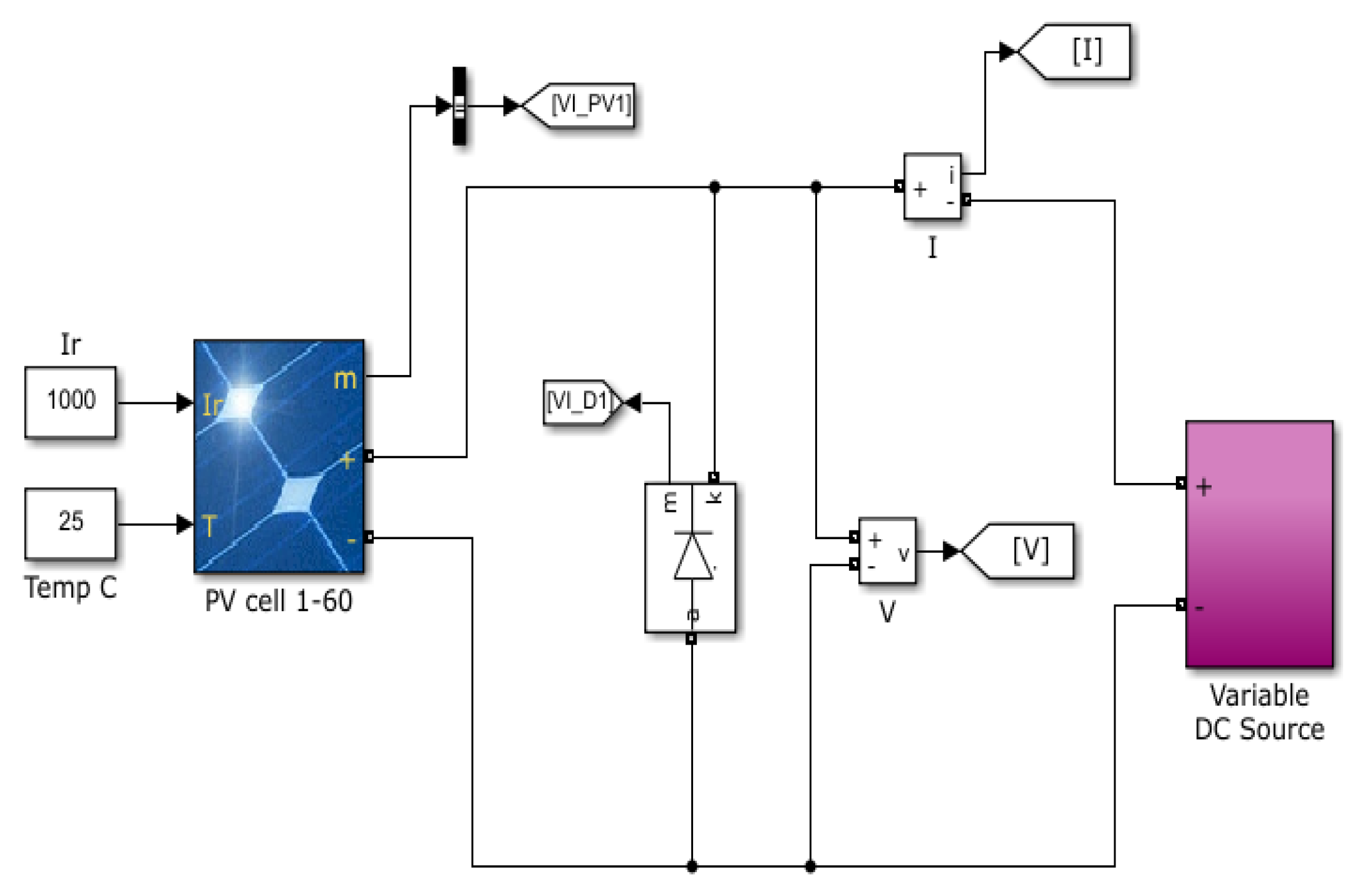
A PV module was created in simulation using MATLAB-Simulink (Figure 2) in order to analyze the impact of various faults on the output of the PV module under standard test conditions (STC). The PV module characteristics were defined to reflect the physical modules used in real-world fault emulation (Table 3). In general, the output of a PV module depends on the inputs to the PV module (namely irradiance and temperature), and PV module parameters. Important PV module parameters are described by PV manufacturers in the PV datasheet. In addition, other features (as listed in Table 4) can be defined to give more detail relating to the operating characteristics of the PV module.
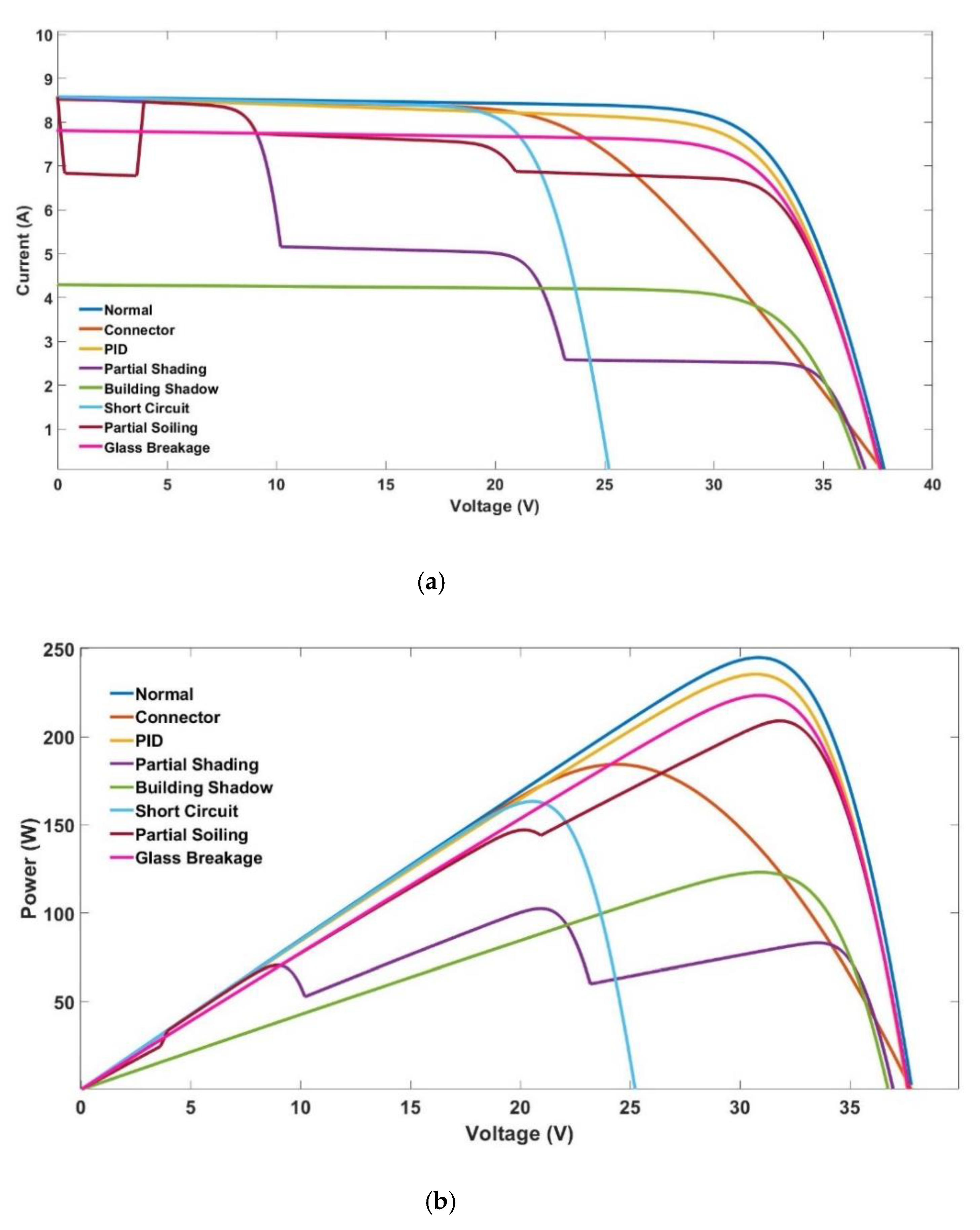
Normal conditions and different faults were simulated, as described in Table 5. For example, for F1 (connector fault), a 1Ω resistor was added in series to the PV system simulation in Figure 2, and for F8 (glass breakage), a 91% irradiance filter was added after the irradiance block. Figure 3 represents the I-V and P-V curves for the PV module that was used for the simulation and experiment under normal and fault conditions. As is clear in Figure 3b, the main impact of the applied faults on the PV output is the reduction of output power. Output power, or power at the maximum power point (MPP), depends on the voltage and current at the MPP. Therefore, these two factors change when different faults occur. The simulation results (Figure 3) show that the most reduction in current at MPP is observed during building shadow. Short circuit current ( Isc ) and open circuit voltage ( Voc ) are two module parameters that are also affected by PV faults. For example, when glass breakage occurs, a decrease in Isc will be clearly observed, and in the case of building shadow, Isc is drastically reduced. Furthermore, open circuit voltage and voltage at MPP ( Vmpp ) are reduced significantly for SC faults compared to the normal operation. All these parameters can be considered as a feature for PV fault detection using machine learning models. Moreover, based on these parameters, other features can be calculated. One such feature is fill factor (FF), which is calculated as follows:
FF = ( I mpp V mpp ) / ( I SC V OC )
where I mpp and V mpp are current and voltage at MPP, respectively.
Based on the literature review and simulation results, FF will reduce when any fault happens in a PV module. However, it is more obvious in the case of partial shading and building shading conditions. In this paper, the impact of different faults on PV module features are investigated and summarized in Table 4. To obtain these results, various simulations were conducted, as well as results from other work, including [3,5,14,23].

3. Experimental Setup

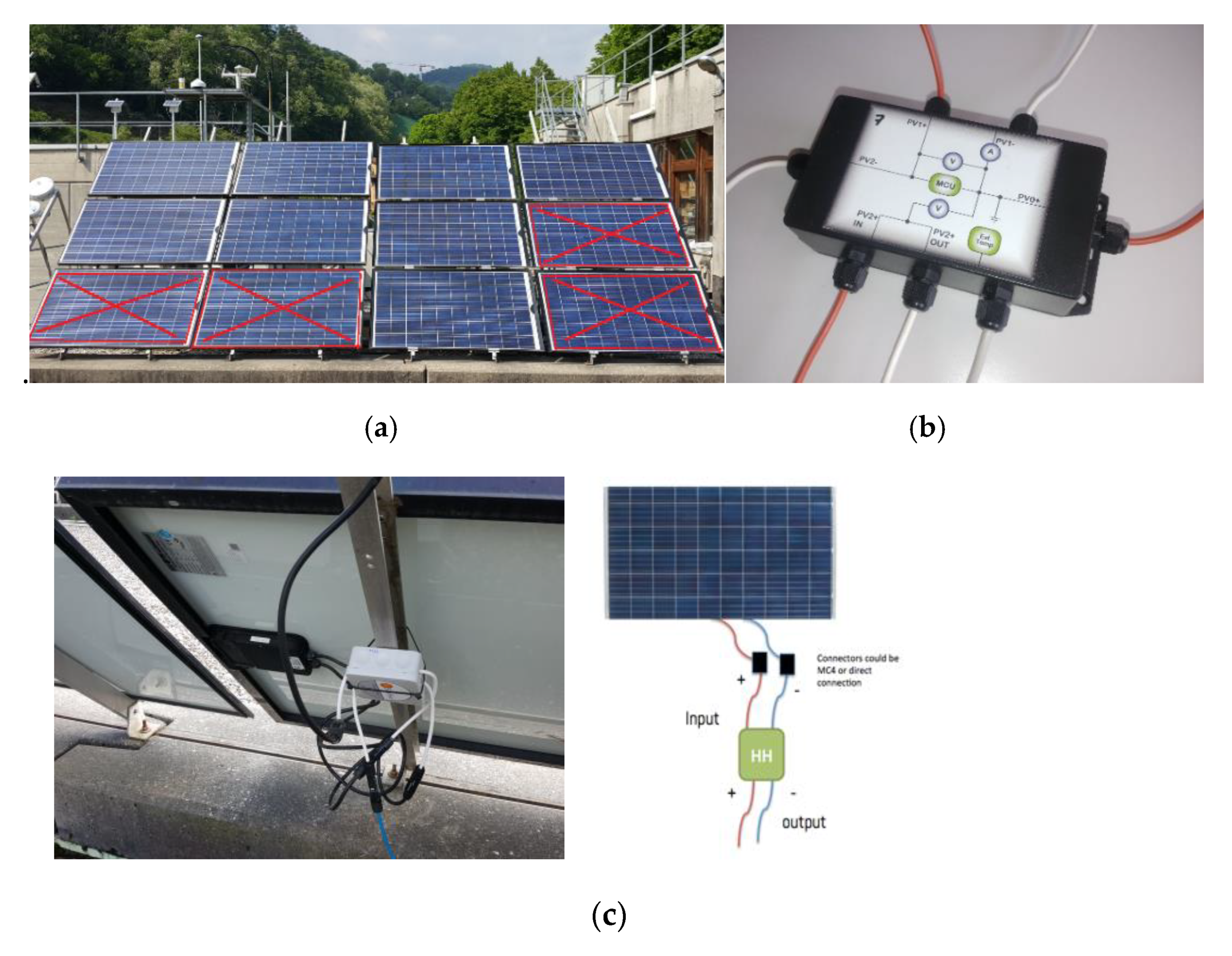
A small-scale grid-connected PV system was set up to create and record current and voltage outputs related to different PV faults under various conditions at the University of Applied Sciences and Arts of Southern Switzerland (SUPSI) in Ticino, Switzerland. This PV system included 12 “SoliTek G/G 245W” PV modules divided into two parallel strings of six in-series modules (Figure 4). Each string was connected to an “SMA Sunny Boy” inverter.
Eight faults plus the normal condition were applied: connector fault (F1), PID fault (F2), partial shading condition/activated bypass diode (F3), pole shading condition (F4), building shading condition (F5), short circuit (F6), soiling (F7), glass breakage (F8), and normal condition (F0). All faults were emulated and implemented according to the descriptions in Table 5. In general, when a PV fault is applied, the PV array may experience some transients and it could operate off its nominal MPP. However, after a few seconds, the maximum power point tracking (MPPT) algorithm will make the PV array operate at a new MPP [24]. This is called the post-fault steady state. Therefore, it is observed that the current and voltage of the PV array at MPP changes depending on the fault condition.
All experiments were undertaken under natural weather conditions; thus, their duration depended on the occurrence of a significant number of clear sky days. Each experiment consisted of at least 8 hours under clear sky irradiance. For collecting data, four HealthHelio (HH) sensors were installed on four modules (Figure 4) to measure voltage, current, and temperature during the summertime from 16 June 2020 to 16 September 2020. The HH sensor is a low-cost device developed by SmartHelio in Lausanne, Switzerland to measure current, voltage, and temperature at a PV module and then transmit the data through a short messaging protocol (e.g., SMS). The HH sensor is a PCB-based IoT device that includes sensors for voltage, current, and temperature, and a microcontroller. Measured data are logged and, in the experimental setup, transmitted to a central cloud-based repository for analysis. Under their commercial model, the information gathered by the sensor is used at the grid edge to assess PV system performance and detect abnormal behavior on the IoT device itself. The data from sensors were combined with irradiance data collected from a local pyranometer to complete the dataset.

4. Feature Extraction and Data Analysis

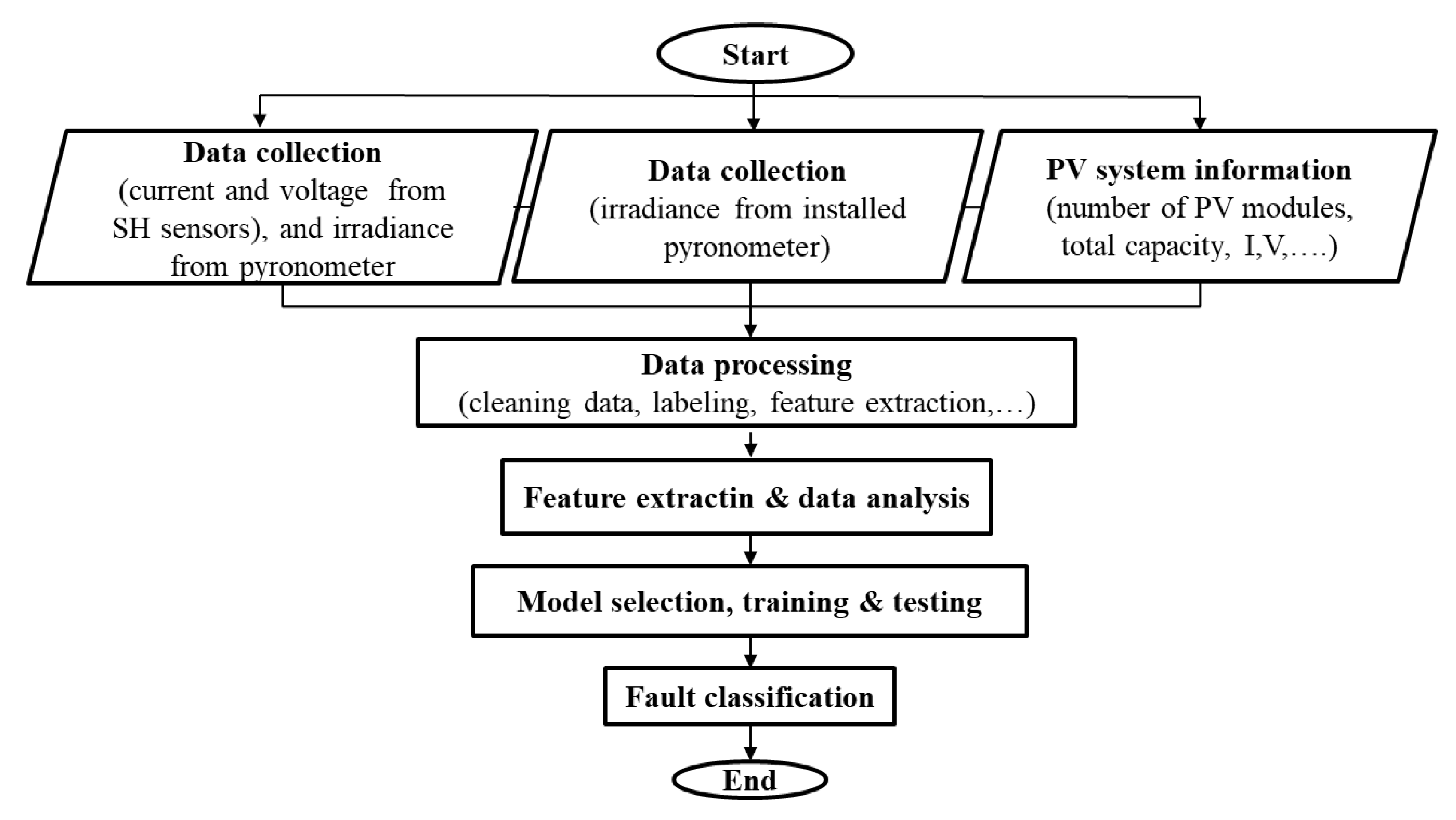
In this research, data collected from the experiment was used to provide a labelled dataset (F0 to F8) that could be utilized to develop a fault detection and classification algorithm. Figure 5 presents a flowchart of the methodology applied for PV fault detection and classification in this paper. The first step is data collection: for this reason, voltage, current, and temperature measurements were collected by the HH sensors, as described in Section 3. The second step of the methodology (Figure 5) is feature extraction and data analysis. A literature study was conducted to identify features that would allow their accurate detection. Based on this study, PV characteristic parameters, information of the installed PV system, and collected data by installed sensors were used to calculate features. Data collected by sensors include PV modules current, voltage, temperature, and average global horizontal irradiance (AGHI). In this research, five features, I / Iexp   (normalized current), V / Vexp   (normalized voltage), P / Pexp (normalized power), V / Voc _ ref , and PV module condition under the experimental test, were selected and calculated for inclusion in a model evaluation. I and V are PV module current and voltage, respectively, that are measured directly by sensors. P is the output power of the PV module that was calculated by the multiplication of current and voltage. Iexp , Vexp , and Pexp are current, voltage, and power under normal conditions, respectively. Voc _ ref is the open circuit voltage of the PV module, which is provided by the PV module datasheet.
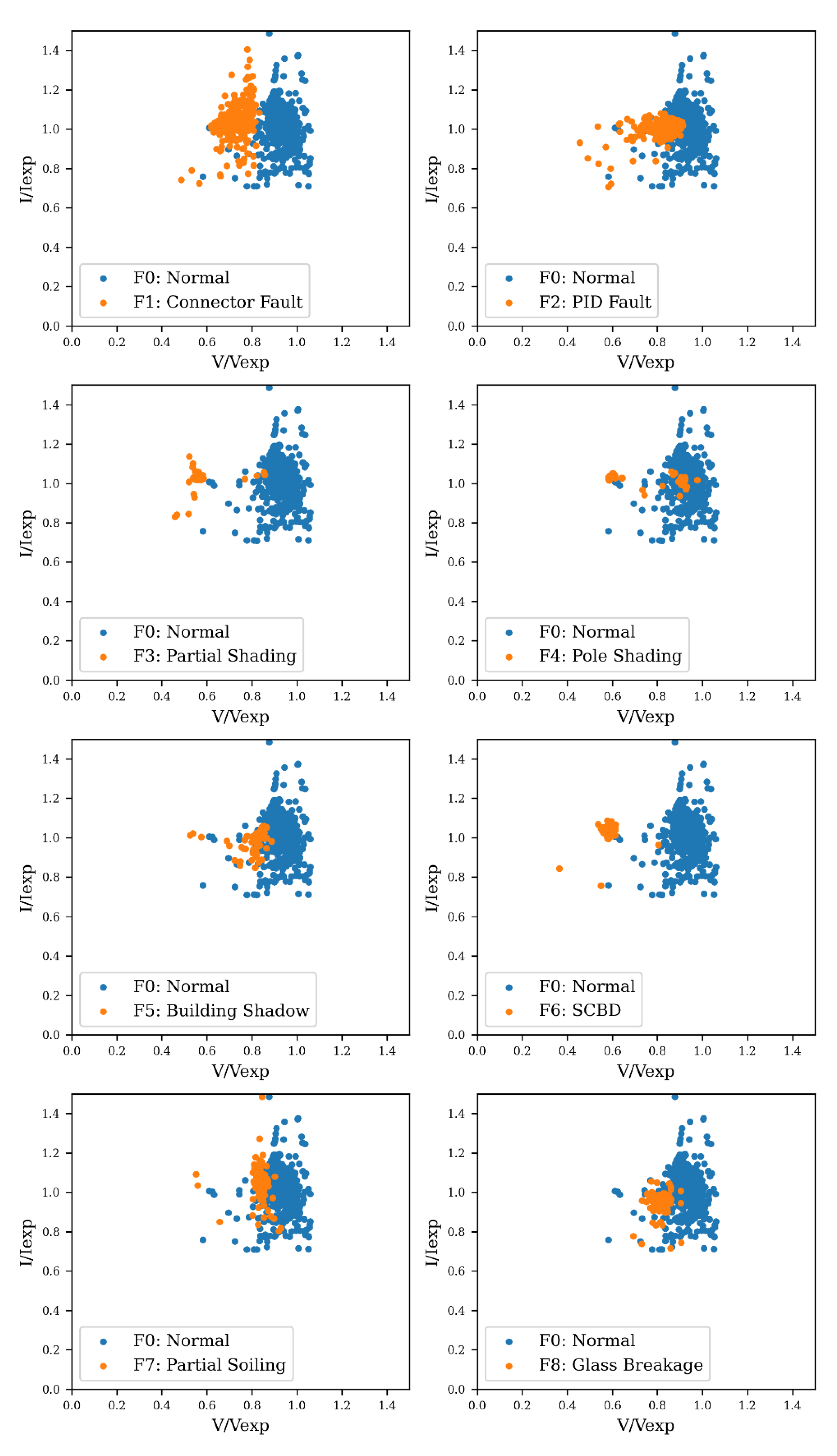
A comparison of the results of data collected from the PV array is provided in this section. Normalized PV module current vs. normalized PV module voltage for each faulty module is compared with healthy module data (also presented as normalized I-V distribution) in one string are shown in Figure 6 and discussed in the following paragraphs. The first fault is corrosion of cell connections or connector fault. It was emulated by adding a 1 Ω resistor in series with the connector. This fault is labeled as F1 (Table 5). It is observed that the connector fault will cause a voltage drop [23] and it can be clearly separated from healthy data. Research in [23] identified that parallel resistance will reduce when a PID fault (F2) is applied. Therefore, to emulate this fault, a 100 Ω resistor is added in parallel to the module. Normalized I-V distribution related to the PID vs normal condition in Figure 6 shows some coincidence of healthy and faulty data. In other words, PID effects are very subtle and not easily observable. This may be due to the emulation methods that were applied in this experiment.
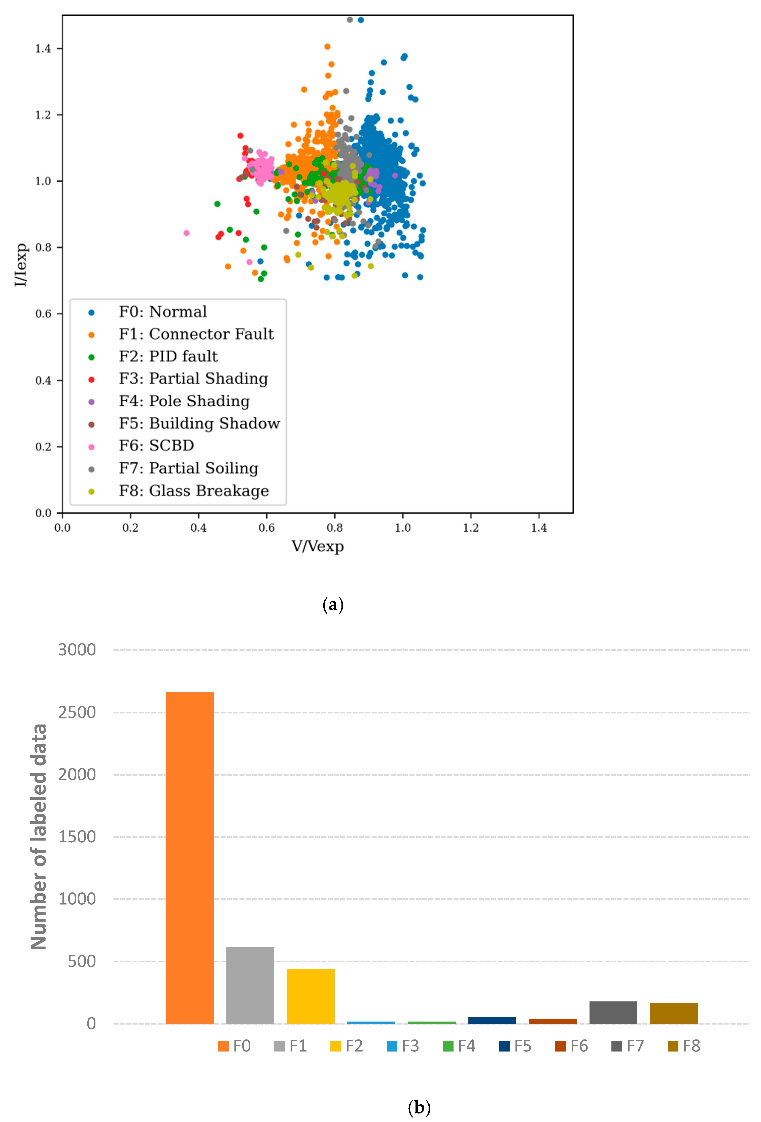
Usually, a difference of 20% between the light hitting the surfaces of different cells in a substring is enough to activate the bypass diode of the substring [1]. This will happen in the case of partial shading, pole shading, or cell crack. In this experiment, a foil was used to activate the bypass diode on the west string. An SC fault can reduce PV array power efficiency by an estimated 22.34 to 27.58% [17]. The results in Figure 6 show that the module voltage drops to two-thirds of the normal module voltage in both partial shading condition (F3) and short-circuited bypass diode (F6), and that they can be clearly differentiated from healthy data. However, this is not the case for pole shading (F4) and building shadow (F5) conditions, as shown in Figure 6. This can be a serious problem for their classification by supervised learning methods, especially when the size of the labeling data is low in these cases (Figure 7b).
In the experiment, soiling was emulated in three different ways: (a) adding a strip over the lower string of cells to emulate partial soiling in a single module, (b) applying a black tape on the lower border of all modules in the west PV string, and (c) using a black band on each one-third portion of each PV module to emulate increasing levels of soiling. The impact of the soiling on the border of all modules is similar to general soiling, i.e., a reduction in current. Soiling in a single module also creates a small voltage drop in the module [23]. The effects can be clearly observed in Figure 6. Finally, foil with a transparency of 91% was used on top of the whole module to emulate a glass breakage fault. The main effect of this fault is current reduction at MPP and a short circuited current (see Table 4). Figure 6 demonstrates that this fault also can be recognized when the output of the PV module is compared with the normal PV module. The normalized (I-V) dataset and the sizing of labeling data for various conditions are given in Figure 7.

5. Fault Detection and Classification

In this section, several supervised learning algorithms were trained and evaluated using the labelled data generated from emulating faults on the PV array at SUPSI. The randomized training set comprised 70% of the collected data, whilst 30% were retained as an unseen test set. Training examples can be denoted as feature and label vectors X and Y, respectively, containing a labeled sample, ( x i , y i ) i = 1 n   X   × Y   , given a set of hypotheses containing functions mapping X to Y, and a loss function representing a non-negative function indicating the deviation between the value predicted by the hypothesis being tested and the true sample. Thus, the goal is to find a hypothesis h with the smallest possible loss as is shown below:
m i n h   ( h ( x ) ,   y ) )
For this reason, seven different supervised machine learning models using the python scikit-learn [25] and TensorFlow frameworks [26] were compared. The baseline model is a multinomial logistic regression model with L 2 regularisation, with the objective function to minimise the cross-entropy loss as calculated by:
L log ( Y , P ) = logPr ( Y | P ) = 1 N i = 0 N 1 k = 0 K 1 y i ,   k log p i ,   k
where for a set of samples, Y represents a 1-of-K binary indicator matrix containing true labels, whereas P is a matrix of probability estimates. The log-loss is computed for all samples in the dataset and parameters updated to minimize L using the limited-memory BFGS optimization algorithm (LM-BFGS) [27]. Next, two Support Vector Machines (SVM) trained with a linear and polynomial kernel of third degree, respectively, both with L 2 regularisation and regularisation parameter C equal to 1. In addition, a K-nearest neighbor (KNN) classifier trained considering five neighbors at each query point, with equal weighting of points in each neighborhood and using Euclidean distance. A single decision tree (DT) classifier was trained, as well as a random forest (RF) classifier with 1000 estimators, with both models using the Gini impurity criterion when evaluating the quality of a split. Finally, a feed-forward neural network (NN) was also trained. The NN comprised two hidden layers (256 and 128 neurons for each layer, respectively, with ReLU activation, and a final softmax activation in the output layer). The model was trained for 500 epochs using minibatch gradient descent with a batch size of 30, the Adam optimizer and sparse categorical cross-entropy as the loss function given by:
1 N i N y i log ( p i )
where N is the number of samples in the minibatch, and y i , and p i represent a one-hot encoded vector of true labels and a vector of softmax output probabilities, respectively.
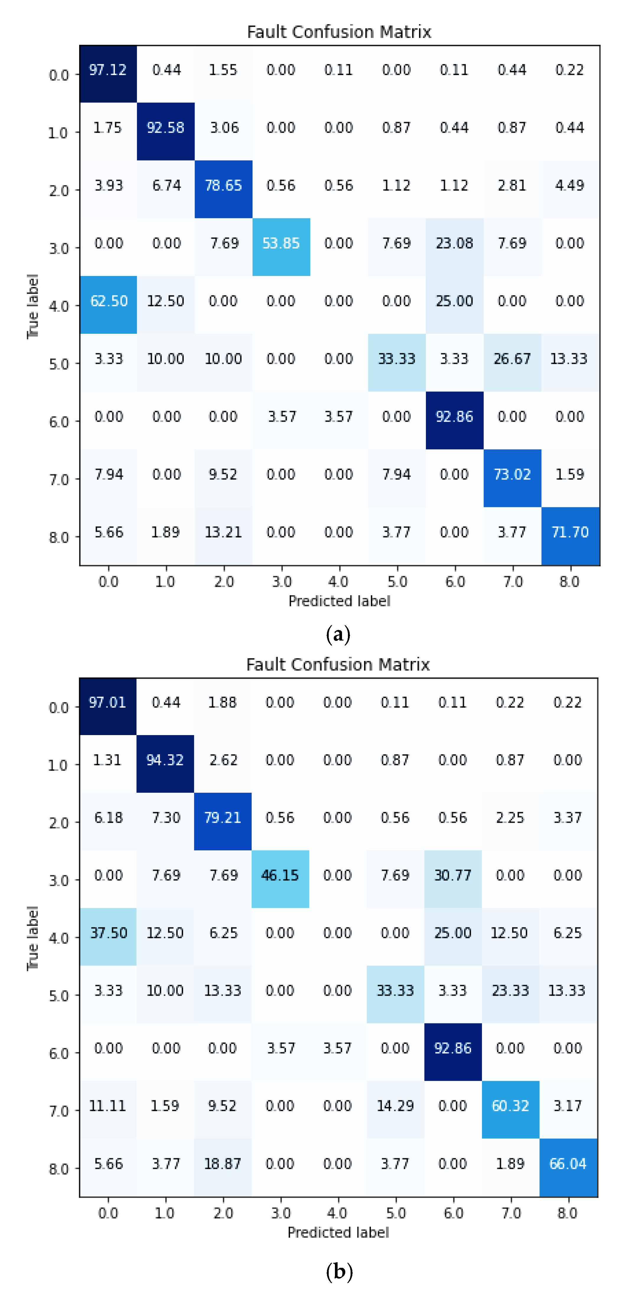
To evaluate model performance on the test set, a variety of accuracy metrics were calculated, and confusion matrices were plotted to demonstrate which models provide the best performance in terms of fault classification. According to the comparison of accuracy metrics, which are represented in Table 6, the RF, KNN, and NN models show the highest performance in terms of accuracy with scores of 89.3%, 88.9%, and 88.6%, respectively. Normalized confusion matrices for these classifiers are plotted in Figure 8b, which shows the fraction of samples correctly classified by each model on a class-label basis. As is clear, 97.12% of all samples belonging to the normal state are correctly classified, whereas for the KNN and NN this is 97.01% and 96.46%, respectively. A similar pattern was observed by computing precision and recall metrics for each model, as can be seen in Table 6, as well as the harmonic mean of those two metrics, the F1 score. Furthermore, the Matthews correlation coefficient (MCC) was also computed for each model, providing an improved metric over the F1 score to quantify model performance on a dataset where classes are imbalanced, as is the case in our dataset. As with the F1 score, the MCC score is highest in the RF model, followed by the KNN and NN models with scores of 0.819, 0.812, and 0.809, respectively.
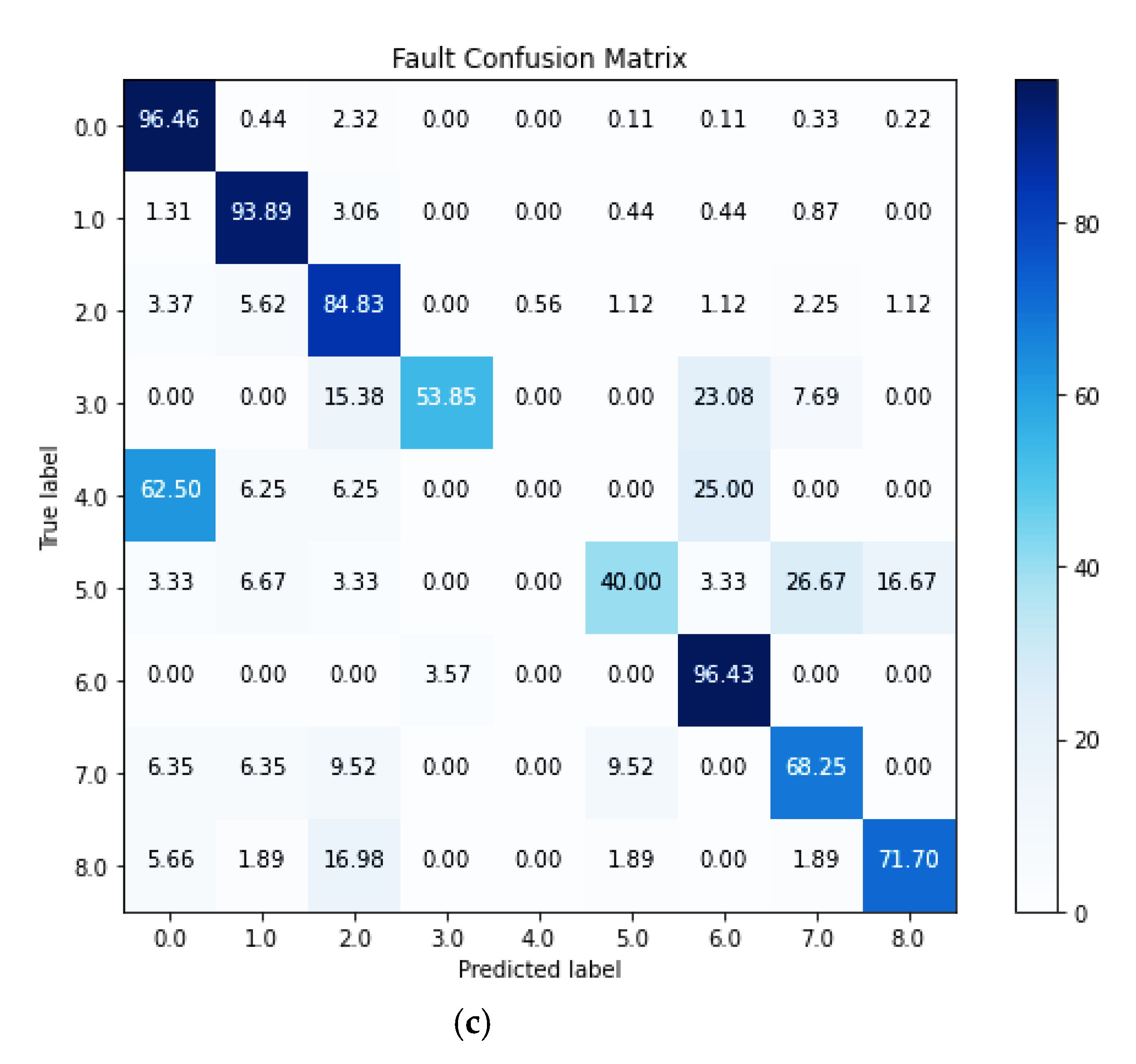
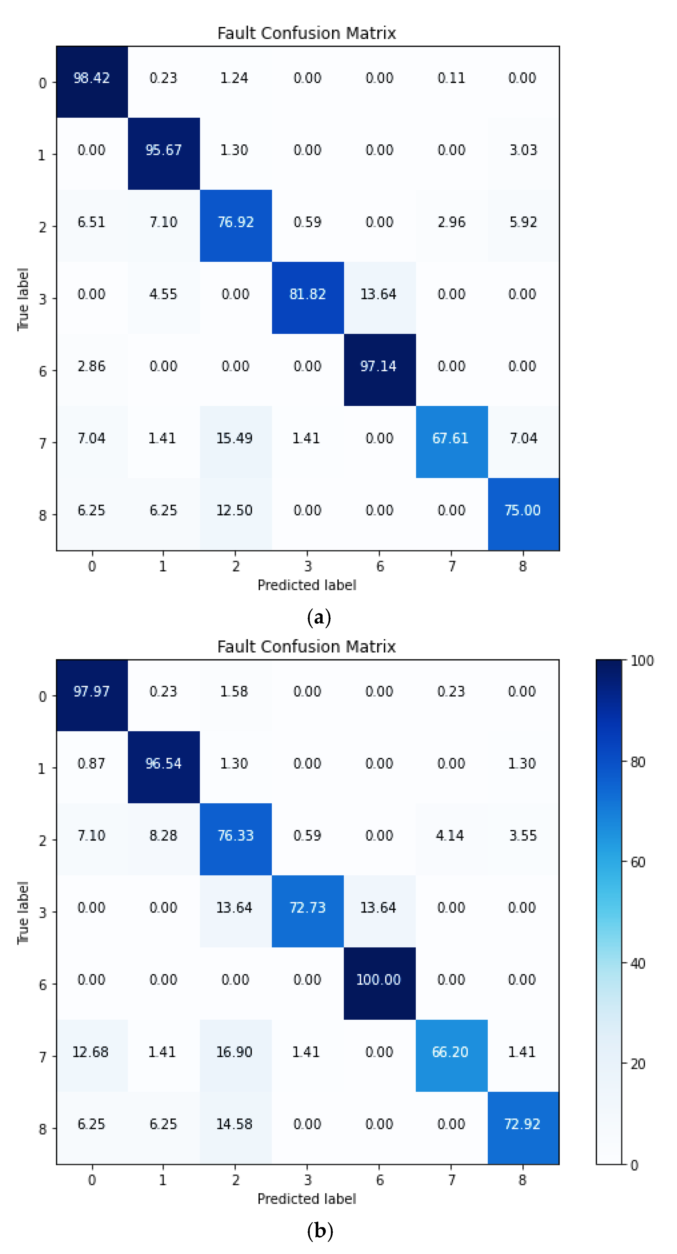
Out of all fault classes, the worst classification performance across all models is seen for pole and building shading conditions. As discussed previously in Section 4, the normalized (I-V) distribution for these two faults is not separated clearly. Moreover, the number of datapoints available for these two faults is very low (Figure 7b), 16 and 52 points, respectively. Therefore, to improve model performance, F4 and F5 were removed from the main dataset and the models retrained and re-evaluated. New accuracy metrics were extracted and are presented in Table 7. As the results show in this table, the NN now shows the highest classification accuracy, F1 score and MCC overall (93%, 0.929, and 0.880), followed by the RF model (92.5%, 0.924, and 0.873). The confusion matrices of these two classifiers are represented in Figure 9. According to the observations from these confusion matrices, both models can identify six faults and the normal state with good predictive performance. The highest fraction of samples correctly classified is achieved by the RF for short-circuit fault (F6) detection at 100%, whilst the lowest fraction of correctly classified samples being 66.2% for soiling fault (F7) detection.
Lower classification performance in some categories may be attributed to the dataset that was used for training. Figure 7b indicates that this dataset is non-uniformly distributed. As is discussed in [28], training ML algorithms on an imbalanced dataset (non-uniform distribution of labels) may lead to a degradation in model performance. It is expected that improved model performance could be achieved with a larger dataset containing more samples of each class. Therefore, additional fault data will be collected for future research to improve the fault classification performance.
According to Table 7, the highest classification accuracy belongs to the NN classifier with an overall 93% accuracy for seven classes. To test the effectiveness of the final classification accuracy obtained by the NN, the proposed method has been compared with the other output results in Table 8. As is shown in this table, different accuracy levels were achieved, ranging from 77.7% to 94% for various fault classifications from different references. Table 8 shows that the network in [3] has a higher accuracy result, but also used a larger dataset. The performance of the proposed NN here would be expected to improve with a larger dataset. Moreover, the network in [3] was trained on MATLAB-based simulation data considering a single isolated module, rather than real-world data from an in-service PV array. Nevertheless, the results in Table 8 prove the achievement accuracy of the proposed method is in an acceptable range compared to the other existing NNs for PV fault detection.

6. Conclusions

In this paper, eight different PV faults were investigated, simulated, and implemented and tested in a real PV system. The purpose of the research was to identify the performance of module-level fault detection and classification to allow the development of a low-cost IoT-based sensor that could be deployed at large scale in low-power-output PV arrays. A panel-level sensor was used to collect current, voltage, and temperature readings at the module level, and then combined with local irradiance readings. This dataset was used to develop ML models that can be used for automatic fault detection and classification at the grid edge. Of all the compared models, the best performing model was found to be the NN. The NN was able to detect six PV faults, plus the normal condition with a classification accuracy on our unseen test set of 93%. However, the classification performance is unsatisfactory for pole shading (F4) and building shading (F5) conditions. The variance in performance is most likely related to the non-uniform distribution of the dataset that was obtained during fault emulation, and the low ratio of these two specific shading conditions (pole and building shading) in comparison to other faults, and the normal state that showed significantly higher detection rates in our study (e.g., up to 100% in some instances). It is expected that classification performance will be improved with the acquisition of additional balanced training data over a larger time horizon and across a variety of different weather conditions. For this purpose, additional data are now being collected for a future study.

Author Contributions

Conceptualization, M.H.; methodology, M.H.; software, M.H.; validation, M.H. and S.K.; formal analysis, M.H.; investigation, M.H.; resources, G.U.; data curation, M.H.; writing—original draft preparation, M.H.; writing—review and editing, M.H., B.B., G.U. and S.K.; visualization, M.H.; supervision, B.B. and G.U.; project administration, B.B.; funding acquisition, B.B. and G.U. All authors have read and agreed to the published version of the manuscript.

Funding

This research was funded by Innosuisse, grant number 45299.1 IP-EE, Intelligent SmartHelio Mesh. The APC was funded by the University of Applied Sciences and Arts (HSLU).

Acknowledgments

The authors would like to thank the University of Applied Sciences and Arts of Southern Switzerland (SUPSI) for the data collection.

Conflicts of Interest

The authors declare no conflict of interest.

References

  1. Samkria, R. Automatic PV grid fault detection system with IoT and LabVIEW as data logger. Comput. Mater. Contin. 2021, 69, 1709–1723. [Google Scholar] [CrossRef]
  2. Fonseca Alves, R.H.; Deus Júnior, G.A.; Marra, E.G.; Lemos, R.P. Automatic fault classification in photovoltaic modules using convolutional neural networks. Renew. Energy 2021, 179, 502–516. [Google Scholar] [CrossRef]
  3. Djalab, A.; Rezaoui, M.M.; Mazouz, L.; Teta, A.; Sabri, N. Robust method for diagnosis and detection of faults in photovoltaic systems using artificial neural networks. Period. Polytech. Electr. Eng. Comput. Sci. 2020, 64, 291–302. [Google Scholar] [CrossRef]
  4. Sun, Y.; Wang, J.; Yang, Q.; Li, X.; Yan, W. Fault Diagnosis of Photovoltaic Module Based on Extreme Learning Machine Technique. In Proceedings of the IMCIC 2018—9th International Multi-Conference on Complexity, Informatics and Cybernetics, Proceedings, Orlando, FL, USA, 13–16 March 2018; Volume 1, pp. 34–39. [Google Scholar]
  5. Eskandari, A.; Milimonfared, J.; Aghaei, M. Fault detection and classification for photovoltaic systems based on hierarchical classification and machine learning technique. IEEE Trans. Ind. Electron. 2021, 68, 12750–12759. [Google Scholar] [CrossRef]
  6. Nieto, A.E.; Ruiz, F.; Patino, D.; Ramirez, O. Classification of electric faults in photovoltaic systems based on voltage-power curves. IEEE Lat. Am. Trans. 2021, 19, 2071–2078. [Google Scholar] [CrossRef]
  7. Zhao, Y.; Lehman, B.; Ball, R.; Mosesian, J.; De Palma, J.F. Outlier Detection Rules for Fault Detection in Solar Photovoltaic Arrays. In Proceedings of the Conference Proceedings—IEEE Applied Power Electronics Conference and Exposition—APEC, Long Beach, CA, USA, 17–21 March 2013. [Google Scholar] [CrossRef]
  8. Zaki, S.A.; Zhu, H.; Yao, J. Fault Detection and Diagnosis of Photovoltaic System Using Fuzzy Logic Control. E3S Web Conf. 2019, 107, 02001. [Google Scholar] [CrossRef]
  9. Mehmood, A.; Sher, H.A.; Murtaza, A.F.; Al-Haddad, K. A diode-based fault detection, classification, and localization method for photovoltaic array. IEEE Trans. Instrum. Meas. 2021, 70, 20987470. [Google Scholar] [CrossRef]
  10. Mehmood, A.; Sher, H.A.; Murtaza, A.F.; Al-Haddad, K. Fault detection, classification and localization algorithm for photovoltaic array. IEEE Trans. Energy Convers. 2021, 36, 2945–2955. [Google Scholar] [CrossRef]
  11. Chine, W.; Mellit, A.; Lughi, V.; Malek, A.; Sulligoi, G.; Massi Pavan, A. A novel fault diagnosis technique for photovoltaic systems based on artificial neural networks. Renew. Energy 2016, 90, 501–512. [Google Scholar] [CrossRef]
  12. Quiroz, J.E.; Stein, J.S.; Carmignani, C.K.; Gillispie, K. In-Situ Module-Level I-V Tracers for Novel PV Monitoring. In Proceedings of the 2015 IEEE 42nd Photovoltaic Specialist Conference, PVSC 2015, New Orleans, LA, USA, 15–19 June 2015. [Google Scholar] [CrossRef]
  13. Khelil, C.K.; Kara, K.; Chouder, A. Fault detection of the photovoltaic System by artificial neural networks. In Proceedings of the 4th International Conference on Green Energy and Environmental Engineering (GEEE-2017), Sousse, Tunisia, 22–24 April 2017. [Google Scholar]
  14. Dhimish, M.; Holmes, V.; Mehrdadi, B.; Dales, M.; Mather, P. Photovoltaic fault detection algorithm based on theoretical curves modelling and fuzzy classification system. Energy 2017, 140, 276–290. [Google Scholar] [CrossRef]
  15. Natarajan, K.; Kumar, B.P.; Kumar, V.S. Fault detection of solar PV system using SVM and thermal image processing. Int. J. Renew. Energy Res. 2020, 10, 967–977. [Google Scholar]
  16. Segovia Ramírez, I.; Das, B.; García Márquez, F.P. Fault detection and diagnosis in photovoltaic panels by radiometric sensors embedded in unmanned aerial vehicles. Prog. Photovolt. Res. Appl. 2022, 30, 240–256. [Google Scholar] [CrossRef]
  17. Jaskie, K.; Martin, J.; Spanias, A. PV fault detection using positive unlabeled learning. Appl. Sci. 2021, 11, 5599. [Google Scholar] [CrossRef]
  18. Bommes, L.; Pickel, T.; Buerhop-Lutz, C.; Hauch, J.; Brabec, C.; Peters, I.M. Computer vision tool for detection, mapping, and fault classification of photovoltaics modules in aerial IR videos. Prog. Photovolt. Res. Appl. 2021, 29, 1236–1251. [Google Scholar] [CrossRef]
  19. Dhimish, M.; Holmes, V.; Mehrdadi, B.; Dales, M. Comparing mamdani sugeno fuzzy logic and RBF ANN network for PV fault detection. Renew. Energy 2018, 117, 257–274. [Google Scholar] [CrossRef] [Green Version]
  20. Bharath Kurukuru, V.S.; Haque, A.; Khan, M.A. Fault Classification for Photovoltaic Modules Using Thermography and Image. In Proceedings of the 2019 IEEE Industry Applications Society Annual Meeting, IAS 2019, Baltimore, MD, USA, 29 September–3 October 2019. [Google Scholar] [CrossRef]
  21. Chen, L.C. Fault Diagnosis and Classification for Photovoltaic Arrays Based on Principal Component Analysis and Support Vector Machine. IOP Conf. Ser. Earth Environ. Sci. 2018, 188, 012089. [Google Scholar] [CrossRef]
  22. Aghaei, M.; Fairbrother, A.; Gok, A.; Ahmad, S.; Kazim, S.; Lobato, K.; Oreski, G.; Reinders, A.; Schmitz, J.; Theelen, M.; et al. Review of degradation and failure phenomena in photovoltaic modules. Renew. Sustain. Energy Rev. 2022, 159, 112160. [Google Scholar] [CrossRef]
  23. SUPSI. SMARTHELIO Innosuisse Check Project; Final Report; Innosuisse: Bern, Switzerland, 2020. [Google Scholar]
  24. Sapountzoglou, N.; Raison, B.A. Grid Connected PV System Fault Diagnosis Method. In Proceedings of the 20th IEEE International Conference on Industrial Technology, Melbourne, Australia, 13–15 February 2019; Available online: https://hal.archives-ouvertes.fr/hal-02072272 (accessed on 30 January 2022).
  25. Machine Learning in Python. Available online: https://scikit-learn.org/stable/ (accessed on 30 January 2022).
  26. TensorFlow. Available online: https://www.tensorflow.org/resources/learn-ml?gclid=Cj0KCQiA09eQBhCxARIsAAYRiymFz-0aitHhd4ubbmbJjW_Ot-YMhiVmzudEVggGw6CR7r9kbWKG2rcaAsSYEALw_wcB (accessed on 30 January 2022).
  27. Morales, J.L.; Nocedal, J. Remark on Algorithm 778: L-BFGS-B: Fortran subroutines for large-scale bound constrained optimization. ACM Trans. Math. Softw. 2011, 38, 2–5. [Google Scholar] [CrossRef]
  28. Sridharan, N.V.; Sugumaran, V. Convolutional neural network based automatic detection of visible faults in a photovoltaic module. Energy Sources Part A Recovery Util. Environ. Eff. 2021, 1–16. [Google Scholar] [CrossRef]
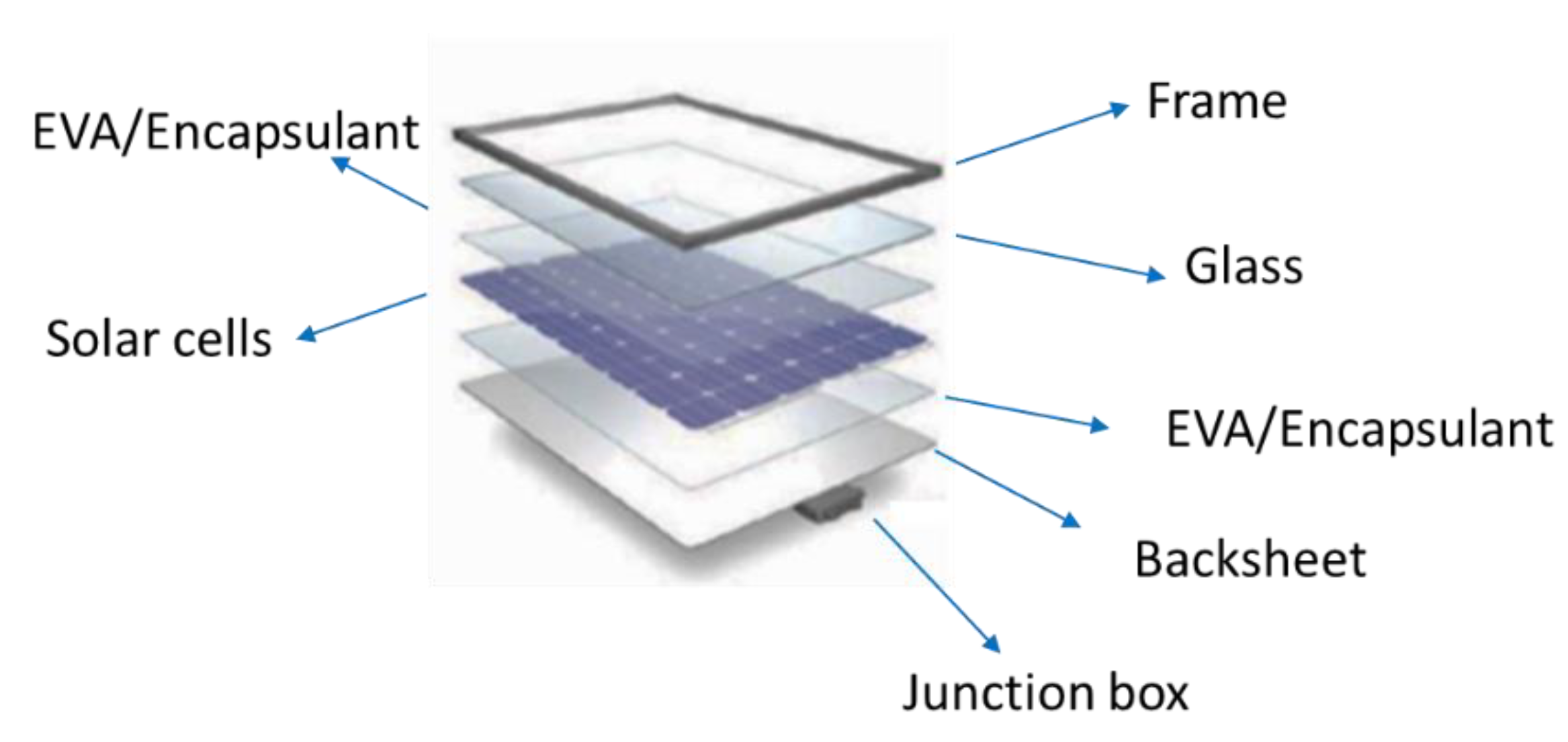
Figure 1. PV module layers [22].
Energies 15 02097 g001
Figure 2. PV system simulation.
Energies 15 02097 g002
Figure 3. PV module outputs under faults and normal conditions: (a) I-V curve, and (b) P-V curve.
Energies 15 02097 g003
Figure 4. Setup of the experimental PV system: (a) PV installation, (b) HH device in the experimental setup, and (c) connecting HH device to the PV module.
Energies 15 02097 g004
Figure 5. PV fault detection and classification flowchart.
Energies 15 02097 g005
Figure 6. Normalized PV module current vs. voltage for various faults compared to the normal condition.
Energies 15 02097 g006
Figure 7. Experiment data distribution: (a) normalized current vs. voltage under various conditions; (b) distribution of labelled data.
Energies 15 02097 g007
Figure 8. Confusion matrices of the three best-performing classifiers trained on all fault data: (a) Random Forest; (b) Nearest Neighbors; and (c) Neural Net.
Energies 15 02097 g008aEnergies 15 02097 g008b
Figure 9. Confusion matrices of the three best-performing classifiers trained on all fault data; (a) Neural Network, and (b) Random Forest.
Energies 15 02097 g009
Table 1. Review of various types of PV fault detection using different methods and technology.
Ref.MethodTechnologyFaultsClassification Accuracy
[15]SVMThermal imageCell crack, soiling, and hot spot caused by shading conditions97
[14]Curve modeling & FUZZYThermal imageDifferent partial shading conditions98.8
[3]ANNElectrical measurement (V, I, and P) in DC sideConnector fault, SC, bypass diode, and partial shading conditions94
[2]CNNThermal imageBypass diode, hot spot, soiling, cell crack, and shading conditions92.5
[13]ANN Impp and Vmpp from measurement & simulationSCNA
[8]Fuzzy
logic control (FLC)
Electrical measurement (V, I, and P) in DC sideSC, OC, and snow coverNA
[18]ResNetThermal IR videoSC, OC, hot spot, PID90
[6]V-PMeasuring and analyzing V-P in AC sideLL, LG, OC94.4
[19]Fuzzy logic and RBF ANNElectrical measurement in DC sideDifferent partial shading conditions92.1
[11]ANNComparing simulation and electrical measurement in DC sidePartial shading conditions, connector fault90.3
[20]ANN, SVM, KNNThermal imageFaulty and normal conditions92.8
[5]Hierarchical
classification
I-V characteristics of PV arrayLL & LG96.66
[7]Outlier detection rulesString currentLL, OC, degradation, and partial shading conditionNA
[21]SVMElectrical measurement in DC sideSC, OC, partial shading conditionNA
[4]RBF-kernel ELMI-V curve tracingSC, OC, degradation, and partial shading conditionNA
[17]Feedback
enhanced MLR (MLRf)
Electrical measurement in DC sideSC, soiling, partial shading conditionNA
[12]Loss factors model (LFM)I-V curve tracingPartial shading condition, degradationNA
[9,10]Diode-based fault detectionVoltage measurement (array voltage, voltage at the positive node of the top and bottom module of a string)LG, LL within a string, LL between two strings and partial shading conditionNA
Table 2. PV module fault classification.
PV Module Faults
PhysicalInternalEVA
Externalconnector
glass breakage
cell crack
degradation/PID
EnvironmentalTemporarydust accumulation
soiling
Permanenthot spot
ElectricalInternalbypass diode faults
open circuit (OC)
Externalline-line fault (LLF)
arc fault
ground fault
Table 3. PV module parameters used in simulation and experiment.
ParameterValue
Pmax 245
Isc 8.58
Voc 37.80
Impp 7.94
Vmpp 30.85
cells per module60
temperature coefficient of Voc −0.34
temperature coefficient of Isc 0.05
Table 4. Impacts of different faults on different PV features.
Type of FaultLabelEffects
IscVocImpVmpRsRshNp 3FFPmax
Connector fault (corrosion of cell connection)F11↓↓2↓↓1↓↓↓↓
PIDF21
Partial shading conditionF3>1↓↓↓↓↓↓
Building shading conditionF5↓↓↓↓↓↓↓↓↓↓1↓↓↓↓↓↓
Failing bypass diode/ short circuit (SC)F6↓↓↓↓↓↓1↓↓↓↓
Partial soilingF7↓↓↓>1
Glass breakageF8↓↓↓↓1
1 and 2 indicate a reduction and increase in the parameter values respectively. 3 is the number of peaks in I-V or P-V characteristic.
Table 5. PV module fault simulation and emulation.
SymbolType of FaultFault SimulationFault Emulation
F1ConnectorConnect 1 Ω resistor in series with the moduleConnect 1 Ω resistor in series with the module
F2PIDAdd 100 Ω resistor in parallel with the PV moduleAdd 100 Ω resistor in parallel with the PV module
F3Partial shading condition/bypass diode activationUse 60% irradiance filter on 1/3 of the PV module and 30% irradiance filter on 1/3 of the PV module Use foil to activate the bypass diode on the west string
F4Pole shading conditionShading with pole on the east string
F5Building shadow conditionAdd a 50% irradiance filter on two PV modules in one stringShadow on two sub-strings in two PV modules
F6Short circuit bypass diodeShort circuit one bypass diodeShort circuit one bypass diode
F7SoilingUse 90% irradiance filter on 1/3 of the module and 80% irradiance filter on 1/3 of the PV module
  • place a strip over the lower string
  • apply black tape on the lower border of all modules
  • use black band on each 1/3 portion of each module
F8Glass breakageApply 91% irradiance filterPlace a foil with 91% transparency on the whole PV module
Table 6. Comparison of the accuracy metrics for supervised algorithms trained and evaluated on the dataset with all faults.
ClassifierAccuracyPrecisionRecallF1Matthews Correlation Coefficient
Random Forest0.8930.8850.8930.8860.819
Nearest Neighbors0.8890.8770.8890.8790.812
Neural Net0.8860.8750.8860.8780.809
Support Vector Machine0.8830.8660.8830.8710.799
Decision Tree0.8640.8630.8640.8630.772
Linear SVM0.8580.8510.8580.8320.758
Logistic Regression0.7440.5860.7440.6490.527
Table 7. Comparison of the accuracy metrics for supervised algorithms trained and evaluated on a dataset without F4 and F5.
ClassifierAccuracyPrecisionRecallF1Matthews Correlation Coefficient
Neural Net0.9300.9300.9300.9290.880
Random Forest0.9250.9240.9250.9240.873
Nearest Neighbors0.9230.9210.9230.9210.869
Support Vector Machine0.9170.9180.9170.9150.860
Decision Tree0.8980.8990.8980.8960.826
Linear SVM0.8920.8950.8920.8780.816
Logistic Regression0.7670.6440.7670.6910.573
Table 8. Comparison of the different results of different references from NN classifier for PV fault detection.
Ref.No. SamplesNo. ClassificationClassification Accuracy %
[20]1568892.8
[3]524281094
[19]7201092.1
[11]1090.3
[19]720577.7
Proposed method4110793
Publisher’s Note: MDPI stays neutral with regard to jurisdictional claims in published maps and institutional affiliations.