A Versatile Model for Estimating the Fuel Consumption of a Wide Range of Transport Modes

Abstract

The importance of a flexible and comprehensive vehicle fuel consumption model cannot be understated for understanding the implications of the modal changes currently occurring in the transportation sector. In this study, a model is developed to determine the tank-to-wheel energy demand for passenger and freight transportation within Germany for different modes of transport. These modes include light-duty vehicles (LDVs), heavy-duty vehicles (HDVs), airplanes, trains, ships, and unmanned aviation. The model further estimates future development through 2050. Utilizing standard driving cycles, backward-looking longitudinal vehicle models are employed to determine the energy demand for all on-road vehicle modes. For non-road vehicle modes, energy demand from the literature is drawn upon to develop the model. It is found that various vehicle parameters exert different effects on vehicle energy demand, depending on the driving scenario. Public transportation offers the most energy-efficient means of travel in the forms of battery electric buses (33.9 MJ/100 pkm), battery electric coaches (21.3 MJ/100 pkm), fuel cell electric coaches (32.9 MJ/100 pkm), trams (43.3 MJ/100 pkm), and long-distance electric trains (31.8 MJ/100 pkm). International shipping (9.9 MJ/100 tkm) is the most energy-efficient means of freight transport. The electrification of drivetrains and the implementation of regenerative braking show large potential for fuel consumption reduction, especially in urban areas. Occupancy and loading rates for vehicles play a critical role in determining the energy demand per passenger-kilometer for passenger modes, and tonne-kilometer for freight modes.

1. Introduction

A 2019 report by the Intergovernmental Science-Policy Platform on Biodiversity and Ecosystem Services found that around one million global plant and animal species are currently under threat of extinction. Some projections suggest that in the coming decades, the global temperature rise will become the single largest agent in the changing of ecosystems globally [1]. In 2019, the German transportation sector accounted for 20.4% of the country’s total emissions of 810 million tonnes of CO₂ equivalent [2]. Germany has set the target of becoming climate-neutral by 2045 [3]. Up until now, the transport sector has shown the least improvement with respect to emissions reduction [4]. Therefore, the sector in Germany is undergoing a massive transformation to meet its climate targets. One of the measures that Germany has taken to reduce its transport sector’s emissions and energy use is subsidizing electric vehicle adaption [5].

To better understand these transformations and their impacts, a model of the energy demand of all possible transportation modes within Germany must be made available. Therefore, this paper aims to develop an approach to determine the vehicle-specific energy demand for passenger and freight transportation. The model can distinguish between the key possible means of transportation available in Germany and the different drivetrains for each transport mode. Additionally, it can consider future developments in energy demand through 2050.

By including light-duty vehicles (LDVs), heavy-duty vehicles (HDVs), aviation modes as well as trains and ships, this paper goes beyond the status of model-based analyses presented in the literature. Moreover, the consideration of varying occupancy and loading rates, as well as the effects of driving conditions, simplifies comparative assessments of the energy demands of all relevant different transportation modes. This is particularly beneficial for projecting future energy demands across the entire transportation sector. The energetic comparison of different transport modes, including the influence of varying occupancy and loading rates, was not present in the literature and is the main outcome of this paper.

The model is divided into on-road and non-road transportation modes. The on-road modes include LDVs and HDVs, which are further subdivided into buses and trucks. The non-road modes include airplanes, unmanned aviation, trains, and ships. Longitudinal vehicle models, in conjunction with efficiency estimates, are used to determine the energy demand for all on-road vehicle modes. Energy demand from the literature is used to build the models for the non-road vehicle modes. The model outputs the energy demand per vehicle-kilometer traveled, as well as the energy demand per passenger-kilometer traveled (for passenger modes) and tonne per kilometer (for freight modes).

In Section 2, a discussion of the models used to determine transport energy demand in the literature is presented in order to determine knowledge gaps and outline the importance of the developed model.

Section 3 presents a detailed description of the developed model for on-road transport energy demand. Section 4 specifies the data preparation and validation, using data from various publications, for the select on-road modes and is followed by a discussion of the non-road modes. Section 5 discusses the different results obtained using the model. It includes multiple parameter variations to analyze their effects on energy demand, as well as a comparison of different transport modes’ energy demands. The paper closes with conclusions drawn from the findings of the study outlined in Section 6.

2. Literature Review

In this section, some of the models in the literature for determining transportation energy consumption are discussed.

2.1. On-Road Transport Modes

In the literature, many ways of modeling vehicle energy demand are reported. One of the most widely used is the longitudinal vehicle energy model. In this approach, the vehicle’s lateral and vertical dynamics are neglected, with the assumption that these do not significantly affect its energy demand [6]. A backward-looking model is used whereby the model starts with the traction energy required at the wheels to follow a driving cycle in order to determine the vehicle’s fuel energy demand [7].

Autonomie is one of the most widely used vehicle simulators and was developed by the Argonne National Laboratory (ANL) in the USA [8]. It is a MATLAB/Simulink-based model library that aims to facilitate the modeling of complex vehicle architectures using “plug-and-play” component models. Autonomie can also be used to study powertrain configurations, control system design, component sizing, parameter tuning, and hardware-in-the-loop, among others [9].

Ahmad et al. (2014) carried out the modeling and validation of the longitudinal vehicle model. The longitudinal model includes different subsystems for tire, engine, automatic transmission, and braking components. It was then validated against an experimental vehicle equipped with embedded sensors. The model results were compared with experimental data for sudden braking and throttle-imposed motions. It was found that the model results were similar to the experimental ones, with an acceptable level of error [10].

Edwardes et al. ([11,12]) utilized the Virginia Tech Comprehensive Power-Based Fuel Consumption Model (VT-CPFM) to model vehicle energy demand. The VT-CPFM employs a longitudinal vehicle model that considers the effects of aerodynamic drag, rolling resistance, inertial effects, and road gradient. Edwardes et al. (2014) modeled diesel and hybrid buses and calibrated their model using publicly available bus information. Incorporating the Orange County bus cycle dynamometer test, the model results had an average error of less than 5% [11]. The authors also modeled diesel buses [12]. Park et al. (2013) validated the VT-CPFM using real-world fuel consumption measurements and calibrated their model using the United States Environmental Protection Agency’s (EPA) city and highway fuel economy ratings [13].

Gao et al. (2007) highlight the need for modeling battery electric vehicles (BEVs) and hybrid electric vehicle (HEVs) [7]. Vagg et al. investigated the modeling of the latter, employing dynamic modeling to optimize the controller and also discussing the disadvantages of dynamic models [14].

Abousleiman et al. [15], Fiori et al. [8], and Luin et al. [16] analyze the energy demand for electric vehicles (EVs). Abousleiman et al. (2015) utilize a longitudinal vehicle model and compare the results obtained with data from driving the modeled vehicle in real-world driving conditions. The impacts of auxiliary loads are also considered with respect to the vehicle’s heating, ventilation, and air conditioning (HVAC) power demands, as well as the power needed for battery conditioning and other drivetrain-related power requirements [15]. Fiori et al. (2016) develop a model to estimate the instantaneous power requirements for EVs based on second-by-second vehicle speed, acceleration, and road grade data as model inputs. The model adopts a quasi-steady-state, backward-looking longitudinal approach due to its fast simulation times [8]. Luin et al. (2019) develop a model to simulate the energy consumption of EVs and use a longitudinal vehicle energy model to determine vehicle energy demand [16].

Several published studies have analyzed the effects of regenerative braking on the energy demand of vehicles. Abousleiman et al. (2015), for instance, use a constant efficiency value to model regenerative braking power [15]. Hayes et al. (2014) assume that if the regenerative power is less than or equal to 20 kW, all of the energy is returned to the battery pack [17]. Fiori et al. (2016) also calculate instantaneous energy regeneration from braking, showing that EVs can regenerate higher energy in urban driving conditions than highway ones [8].

Ambient temperatures can affect the energy demand of vehicles through various mechanisms. The HVAC system for the passenger compartment is one of the major consumers. Fiori et al. (2016) consider the effects of auxiliary systems such as air conditioning and heating systems and demonstrate that the use of HVAC systems can reduce the EV range [8]. Abousleiman et al. (2015) model HVAC power requirements using a function that varies with the ambient temperature. According to this model, the power demand for cabin HVAC is negligible for ambient temperatures between approximately 14 and 27 °C [15]. In turn, Grube et al. (2018) utilized a simplified thermal model to determine the vehicle cabin’s HVAC energy requirements [18].

Ambient temperatures also affect fuel consumption when the engine is started at temperatures lower than its normal operating ones, which is known as a cold start. Bielaczyc et al. (2011) experimentally determine the effects of low ambient temperatures on the cold-start emissions and fuel consumption of various spark ignition and compression ignition passenger vehicles across the New European Driving Cycle (NEDC). The fuel consumption was found to be approximately 20% higher at an ambient temperature of −7 °C compared to 24 °C above the NEDC from cold starts [19]. In addition to the ambient temperature, the effects of cold starts also depend on various other parameters, including the volume of the engine, the type, and the elapsed time since its last use. The effects of cold starts are not considered in this model due to the large number of parameters that affect fuel consumption during cold starts.

Various studies have analyzed the effects of different standard driving cycles in order to determine fuel demand for passenger vehicles. Grube et al. (2018) analyzed the impact of driving cycles and auxiliary power on passenger cars’ fuel energy demand. The analysis included internal combustion engine vehicles (ICEVs), HEVs, BEVs, and fuel cell electric vehicles (FCEVs) and focuses on reducing fuel consumption using electric power [14]. Duarte et al. (2016) compared real fuel consumption from on-road data with those obtained under standard driving conditions for vehicle certification. The findings revealed that on-road fuel consumption levels were 23.9% and 16.3% higher, respectively, than the results obtained using the NEDC and Worldwide Harmonized Light Vehicles Test Procedure (WLTP) Class 3 cycle [20]. This highlights the discrepancy between the certified and real-world fuel economy of vehicles and shows that the newer WLTP standard is closer to the real world than the older NEDC.

2.2. Non-Road Transport Modes

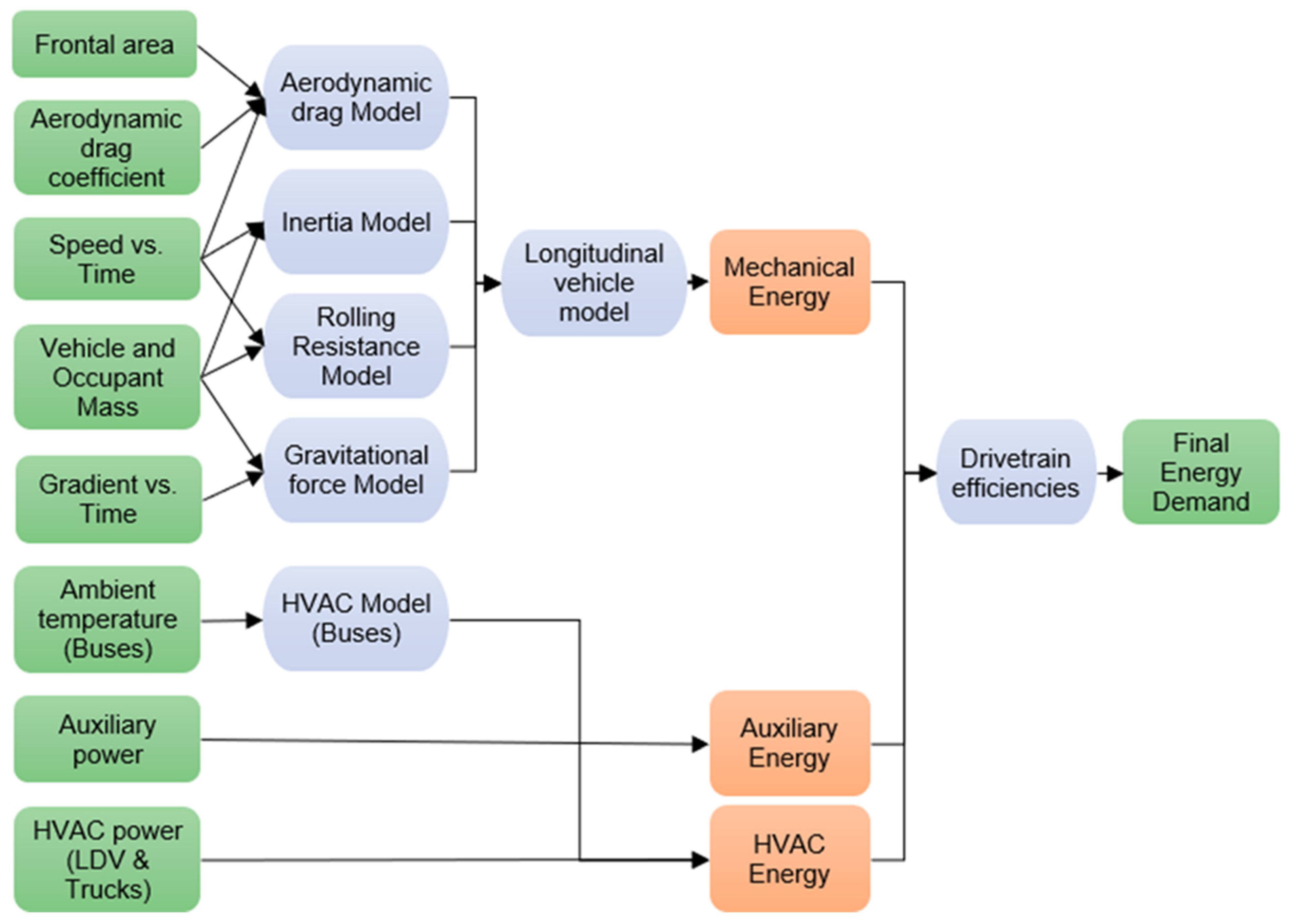
Between 1990 and 2018, international aviation saw the highest relative increase, at 124.6%, compared to other transportation modes, in terms of energy consumption within the EU [21]. Globally, aviation was responsible for 2.8% of all CO₂ emissions from fossil fuel combustion in 2019 [22]. Therefore, airplane fuel energy demand must be considered in any holistic model of the transport sector.

Burzlaff (2017) develops a model for determining aircraft fuel consumption that can evaluate type-specific fuel consumption using publicly available airplane information [23]. Park et al. (2014) model the airplane fuel burn for different models globally and find that flight lengths of between 1500 and 2000 nautical miles are the most fuel-efficient [24].

Peeters et al. (2005) assess the change in commercial airplanes’ fuel efficiency from the 1930s to the 2000s [25]. In turn, Kharina et al. (2015) discuss the fuel efficiency trends for airplanes from 1960 to 2014 [26].

Xu (2017) models the energy demand of differently sized freight unmanned aviation [27]. Meanwhile, Bauhaus Luftfahrt determines the energy demand for passenger unmanned aviation [28].

The energy demand for railways must be further evaluated in order to save energy on the back of environmental concerns and high energy costs [29].

Salvador et al. (2018) develop a dynamic model for estimating the energy consumption of diesel trains. A comparison of the model results against real operational data reveals an error rate of less than 9% [30].

Wang et al. (2017) build a model for determining the energy consumption of electric trains. The model is calibrated using data from Oregon in the United States and validated using data from the National Transit Database. The model’s results are sufficiently accurate and show that the use of regenerative braking can reduce energy consumption by around 20%. The model can also take into account the effects of train models, routes, and operational parameters [31].

The shipping industry is responsible for transporting the vast majority of global trade volumes [32]. Jeon et al. (2018) predict ships’ fuel consumption by employing artificial neural networks to analyze big data collected from ships. The paper reports this method as being more accurate and efficient than polynomial regression and support vector machines [33].

Yang et al. (2019) model the fuel consumption for ships using a genetic algorithm-based grey-box model, whose advantages over other grey-box models include that it can better account for oblique weather directions [34].

One of the main differences between the model being developed in this paper and those presented in the literature is the number of different modes of transport included. Germany’s different transport modes must be modeled in order to obtain an overview of the German transport network’s energy demand. Most models to be found in the literature only simulate specific transport modes. The model developed in this paper incorporates LDVs, HDVs (buses and trucks), aviation modes (including conventional fixed-wing airplanes and electric unmanned aviation), trains, and ships. These modes are further subdivided into passenger and freight classifications. Therefore, a single model can be easily used to determine the energy demand for any transport mode, which simplifies the applicability of the model to complex projects. Another specialty of this model is that it can analyze the effects of different occupancy rates, i.e., the energy requirements for transporting each passenger, or a tonne of cargo, can be analyzed. The model also considers the effects of driving conditions such as ambient temperatures and driving scenarios for on-road transport modes. This simplifies the comparison of energy demand between different modes of transport and facilitates a parameter analysis.

3. Methodology

This section outlines the physics behind the implemented model used to determine the on-road vehicle’s mechanical energy demand, followed by a discussion of the effects of regenerative braking systems and the model used to determine the vehicle’s final fuel energy demand.

The physics behind the simulation used for on-road vehicles are extensively discussed and will also be the most detailed aspect of the final model. This is undertaken because German road transportation underlies approximately 90% of the country’s entire transport sector energy demand, with only cars and light trucks accounting for 63.0% for the year 2017 [35].

A vehicle’s drivetrain converts the energy stored in the fuel into mechanical energy, which is then used to overcome driving resistances. There are three main types of driving resistances [36]:

• Aerodynamic friction;
• Rolling friction;
• Energy dissipated by braking.

These resistances can be represented in a differential form, as follows:

$$m_{e,v}\frac{d}{dt}v\left(t\right)=F_{trac}\left(t\right)-\left(F_a\left(t\right)+F_r\left(t\right)+F_g\left(t\right)+F_d\left(t\right)\right)$$

(1)

where:

$F_a$ = aerodynamic friction;

$F_r$ = rolling friction;

$F_g$ = gravitational force for non-horizontal roads;

$F_d$ = disturbance forces;

$F_{trac}$ = traction force at the wheel;

$m_{e,v}$ = equivalent mass of the vehicle and its occupants;

$v$ = speed of the vehicle.

This model is referred to as the longitudinal vehicle model because it only considers the dynamics with respect to the vehicle’s longitudinal axis. It does not consider the lateral forces affecting it.

Equation (1) conveys a general overview of the energy pathways of a vehicle. $F_d$ represents any external forces acting on the vehicle. $F_{trac}$ is the force being generated at the wheelbase to propel the vehicle. The effects of vertical lift force are neglected.

The aerodynamic friction, rolling resistance, and gravitational forces are calculated thus [36]:

$$F_a\left(v\right)=\frac{1}{2} · {\rho }_a · A_f · c_a · v^2$$

(2)

$$F_r=c_r · m_v · g$$

(3)

$$F_g\left(\alpha \right)=m_v · g · \mathsf{\alpha }$$

(4)

where $v$ is the vehicle speed, ${\rho }_a$ is the density of the air, $A_f$ is the frontal area, $c_a$ is the aerodynamic drag coefficient, $m_v$ is the vehicle’s mass, along with passengers and cargo, $g$ is the gravitational acceleration, and $\alpha$ is the road gradient.

The rolling resistance $c_r$ is assumed to be dependent on the vehicles’ speed alone [37].

$$c_r=0.0088+0.0017 · \frac{v}{100}+0.00028 · {\left(\frac{v}{100}\right)}^4$$

(5)

Equation (S1) is used to determine the equivalent vehicle mass $m_{e,v}$ (see the Supplementary Information). Multiplying the equivalent vehicle mass by the vehicle’s acceleration yields the force required for the vehicle’s acceleration, also known as the motive force [38].

Traction force is that which the wheel must exert on the road to propel the vehicle against the resisting forces. A no-slip condition is assumed to hold between the tire and road. Thus, the wheel’s torque is fully transferred to the road [39].

Therefore, to determine the traction force, the driving mode must first be determined. There are three possible driving conditions [36]:

• Traction mode—the engine is doing the work of moving the vehicle;
• Braking mode—the brakes are dissipating energy to slow down the vehicle;
• Coasting mode—the vehicle is moving under its own stored mechanical energy.

The vehicle’s coasting velocity can be calculated using Equation (1), assuming no disturbance force and setting the traction force to zero. It results in the following equation for calculating the coasting velocity [36]:

$$\frac{d}{dt}{v}_c\left(t\right)=\frac{-1}{2 · m_{e,v}} · {\rho }_a · A_f · c_a · v_c^2\left(t\right)-g · c_r-g · \alpha$$

(6)

The above equation can be easily solved using a numerical method—in this case, the forward Euler method [40]. By comparing the result with the actual vehicle velocity $v\left(t\right)$ during the driving cycle, the driving mode can be determined [36].

A vehicle is in traction mode if $v\left(t\right)>v_c\left(t\right)$, in braking mode if $v_c\left(t\right)>v\left(t\right)$, and in coasting mode if $v_c\left(t\right)=v\left(t\right)$, for a finite time interval.

According to this model, the vehicle speed and road gradient must be predetermined to determine the wheels’ traction force. The predetermined speed is provided by the standard driving cycles, which are discussed in Section 4.1.1.

The vehicle’s mechanical energy demand is the energy that the vehicle requires to follow the chosen driving cycle. The key parameter used in this calculation is the mean tractive force, ${\overline{F}}_{trac}$. The mean tractive force is defined as:

$${\overline{F}}_{trac}=\frac{1}{x_{tot}} · {{\displaystyle \int }}_{t \in trac}^{}F\left(t\right) · v\left(t\right)dt$$

(7)

where $trac$ is the time intervals in which $F_{trac}>0$—in other words, those parts of the cycle when the vehicle is in traction mode—and $x_{tot}$ is the total distance traveled during the cycle.

During the parts of the driving cycle when the vehicle is in the braking ($F_t<0$) or coasting modes ($F_{trac}=0$), it does not require any mechanical energy from the drivetrain. The energy needed for aerodynamic and rolling resistances is provided by the decrease in the vehicle’s mechanical energy.

Next, the 0% and 100% brake energy recuperation scenarios are considered.

If the vehicle is not fitted with a braking energy recuperation device, Equation (1) is applicable. Thus, there are four significant contributions to the traction force:

$${\overline{F}}_{trac}={\overline{F}}_{trac,a}+{\overline{F}}_{trac,r}+{\overline{F}}_{trac,m}+{\overline{F}}_{trac,g}$$

(8)

Please refer to the Supplementary Information for a detailed breakdown of Equation (8) and further discussion on the effects of recuperation efficiency.

As 100% efficiency is not feasible in a real-world scenario, the model will interpolate the actual energy demand based on the “No Recuperation” and “Perfect Recuperation” energy demands:

$${\overline{F}}_{trac}\left({\eta }_{rec}=rec\right)={\overline{F}}_{trac}\left({\eta }_{rec}=100\%\right)+\left(1-rec\right) · \left({\overline{F}}_{trac}\left({\eta }_{rec}=0\%\right)-{\overline{F}}_{trac}\left({\eta }_{rec}=100\%\right)\right)$$

(9)

where ${\eta }_{rec}$ is the recuperation efficiency, $rec$ is the actual recuperation efficiency of the vehicle as a fraction, ${\eta }_{rec}=0\%$ is the “No Recuperation” scenario, ${\eta }_{rec}=100\%$ is the “Perfect Recuperation” scenario, and ${\eta }_{rec}=rec$ is the scenario for the given recuperation efficiency.

Finally, the mechanical energy demand $E_{mech}$ of the vehicle is calculated based on the mean tractive force, which is equal to the average energy consumed per distance traveled. When the mechanical energy demand is expressed in units of MJ/100 km, the relationship between the quantities is as follows:

$$E_{mech}={\overline{F}}_{trac} · v · h$$

(10)

After calculating the vehicle’s mechanical energy demand, the next major sources of energy demand must be considered. These include the power needed for the vehicle’s HVAC system and other essential components. In this model, these systems are combined into one and referred to as the auxiliary power $P_{aux}$ demand, which is used as an input. The auxiliary energy $E_{aux}$ demand is then calculated as follows:

$$E_{aux}={\displaystyle \sum }_{i=1}^n{P}_{aux} · h$$

(11)

where $h$ is the time interval between the discrete data points and the summation is carried out throughout the driving cycle. Therefore, the energy provided by the drivetrain is the summation of the $E_{mech}$ and $E_{aux}$ demand of the vehicle. The drivetrain efficiencies are then applied to the summation of the mechanical and auxiliary energy demands to determine the final fuel energy demand for the vehicle.

Figure 1 shows the structure of the model developed to determine the energy demand for the on-road transport modes.

In cases where the vehicle has two different energy stores or motors, the mechanical and auxiliary energy demands are shared based on the driving share ratios. The final fuel energy demands are then calculated separately for individual storage and the motor.

4. Data Preparation and Validation

In this section, the data used to build the model are discussed. The validation of the model’s elements is also discussed.

4.1. On-Road Transport Modes

This section outlines the data used to build the on-road vehicle models.

4.1.1. Standard Driving Cycles

Standard driving cycles are the speed versus time profiles that aim to mimic real-world vehicle operation [41]. The Worldwide Harmonized Light Vehicles Test Cycle (WLTC) was developed to provide better laboratory estimates for real-world vehicle emissions and fuel consumption for LDVs [42].

The WLTC Class 3b is divided into four distinct driving scenarios, namely low, medium, high, and extra-high speed regions, representing urban, suburban, rural, and highway scenarios, respectively. Figure 2 shows the driving cycle [42].

As can be seen from Figure 2, the driving cycle features distinct driving characteristics for the four different scenarios. WLTC Class 3b is used by the default to model the energy demand of all LDVs. Other driving cycles are also made available within the model to simulate different driving conditions.

4.1.2. Light-Duty Vehicles

LDVs are subdivided into five modes: small car, medium car, large car, sport utility vehicles (SUVs), and light commercial vehicles (LCVs). The different modes are identified on the basis of EC regulation number 4064/89 [43]. The different modes and their EC classifications are displayed in

Table 1. LDV modes’ EC classification and the average aerodynamic parameters.

Mode	EC Classification	${\mathit{A}}_{\mathit{f}}$ (m2)	${\mathit{c}}_{\mathit{a}}$ (-)
			2020	2030	2040	2050
Small Car	A and B	2.16	0.309	0.286	0.245	0.239
Medium Car	C	2.25	0.271	0.251	0.215	0.210
Large Car	D	2.21	0.262	0.242	0.208	0.203
SUV	J	2.45	0.327	0.302	0.259	0.253
LCV	M	3.17	0.349	0.322	0.276	0.270

.

The top 30 best-selling vehicles in Germany for the year 2019 were researched to find their aerodynamic drag coefficients $c_a$ and frontal areas $A_f$. The average values were assumed to be for the year 2020. Islam et al. (2020) predict the percentage drag coefficient reduction through 2050 [44]. The average mode-specific values for each decade are presented in Table 1.

Table 2. Drivetrain efficiencies for LDVs, based on data from different sources.

Drivetrain	2020	2030	2040	2050	Sources
ICEV-g	0.26	0.31	0.34	0.36	[44,46,47]
ICEV-d	0.27	0.36	0.39	0.40	[44,46,47]
HEV-g	0.30	0.35	0.38	0.40	[44,45,46,47]
HEV-d	0.31	0.40	0.43	0.44	[44,45,46,47]
PHEV-g	0.30	0.35	0.38	0.40	[44,45,46,47]
PHEV-d	0.31	0.40	0.43	0.44	[44,45,46,47]
PHEV-fc	0.47	0.52	0.56	0.59	[44,46,48,49,50]
REEV-g	0.30	0.35	0.38	0.40	[44,45,46,47]
REEV-d	0.31	0.40	0.43	0.44	[44,45,46,47]
REEV-fc	0.47	0.52	0.56	0.59	[44,46,48,49,50]
BEV	0.75	0.81	0.85	0.87	[44,46,48,49,50]
FCEV	0.47	0.52	0.56	0.59	[44,46,48,49,50]
ICEV-cng	0.26	0.31	0.34	0.36	[44,46,47]

shows all the different drivetrain efficiencies that are applicable for LDVs. Hybrid drivetrain efficiency is assumed to be 4% higher than its conventional counterpart [45]. Hybrid vehicles are divided into electric and conventional/fuel cell modes. In our model, efficiencies are assumed to be constant. This simplification was chosen to make the model more flexible regarding scenario calculations and sensitivity analyses. In reality, however, efficiency is a function of the powertrain’s load spectrum, which is specific for driving cycles and would also include the consideration of onboard auxiliary loads, such as air conditioning.

The recuperation efficiency is determined based on the electric drivetrain efficiency, which is responsible for recuperating the braking energy. The electric drive shares for PHEVs and REEVs are taken to be a function of their yearly driven distance [51]. The average occupancy for all LDVs is assumed to be 1.3 passengers per vehicle, which is the average value for Germany [52].

The density of air ${\rho }_a$ is taken as 1.225 kg/m³, assuming a temperature of 15 °C and standard atmospheric pressure [53]. This is used for all LDV and HDV modes.

According to the European Union’s Aviation Safety Agency, the European average passenger weight is 83 kg, which includes the mass of a person and accompanying luggage [54]. This is used for all LDV and HDV modes.

4.1.3. Buses

A similar analysis was carried out for the other on-road modes. For buses, an additional model is built to determine their auxiliary power demand as the auxiliary power of buses can be a significant portion of the total fuel consumption. This is especially true when HVAC power is required during extreme weather conditions. Cox (2018) reports an average power rating of 13.05 kW for a medium bus with, and 6.15 kW without, HVAC power demand [55]. Since the HVAC power demand for buses is significant, it was decided to consider it in more detail. Knote et al. (2017) report the HVAC energy consumption per distance traveled as a function of the ambient temperature for medium buses. Figure 3 shows this relation for different cruising velocities [56].

The HVAC energy consumption values shown in Figure 3, reported for ambient temperatures between −4 °C and 17 °C, approximately, are assumed for medium buses. HVAC energy is assumed to be the same for lower ambient temperatures as the one for −4 °C and the same as for 17 °C for higher temperatures. This is assuming that, at lower temperatures, the HVAC system has reached its power limitations. For higher temperatures, the HVAC system still needs to maintain ventilation functions, for which the minimum energy is required. However, the model is best suited to estimate energy needs within the specified range of ambient temperatures.

4.1.4. Validation

Here, the model results for the ICEV, FCEV, and BEV drivetrains of the chosen modes are compared with data from the literature and real vehicles to confirm the model’s validity.

Figure 4 shows the ICEV-g, FCEV, and BEV energy demands of medium cars as predicted by the model compared to energy demand data reported for various vehicle manufacturers.

As can be seen from Figure 4, the model results are in good agreement with the values reported for real vehicles in the market. The Pearson correlation coefficient between the model results and those reported for real vehicles is 0.953 for ICEV-g and 0.952 for BEVs, which represents a high degree of correlation. Due to the lack of sufficient datapoints for FCEVs, it was not possible to calculate a valid correlation coefficient; however, the model results fall within the range of reported data for real vehicles.

Next, the results for buses and trucks are validated using data reported for current vehicles in the literature. Due to their prominence, medium buses and large trucks are chosen to represent their respective modes. The results for medium buses (Figure 5) and large trucks (Figure 6) are validated using data reported for the current vehicles in the literature.

In Figure 5 and Figure 6, the range of values is shown by the shaded region representing the energy demand for different occupancy rates for buses and loading rates for trucks. The solid line indicates the energy demand for the average occupancy rate in Germany. As can be observed, the results from the model match well with those reported in the literature.

If the literature data are assumed to be normally distributed, the fraction of literature data falling within the range of model results can be determined. In Figure 5, 65% of BEV, 99% of FCEV, and 75% of ICEV-d literature data fall within the range of the model results. In contrast, in Figure 6, 98% of BEV, 100% of FCEV, and 85% of ICEV-d literature data fall within the scope of the model results. As none of the literature mentioned the occupancy/loading rates for the vehicles, it is difficult to determine the sources of the fluctuations. However, for each drivetrain, for buses and trucks, the average of the literature data falls within the range of model results. Additionally, all of the FCEV literature data are within the range of the model results. Therefore, it can be concluded that the model results are valid.

4.2. Non-Road Transport Modes

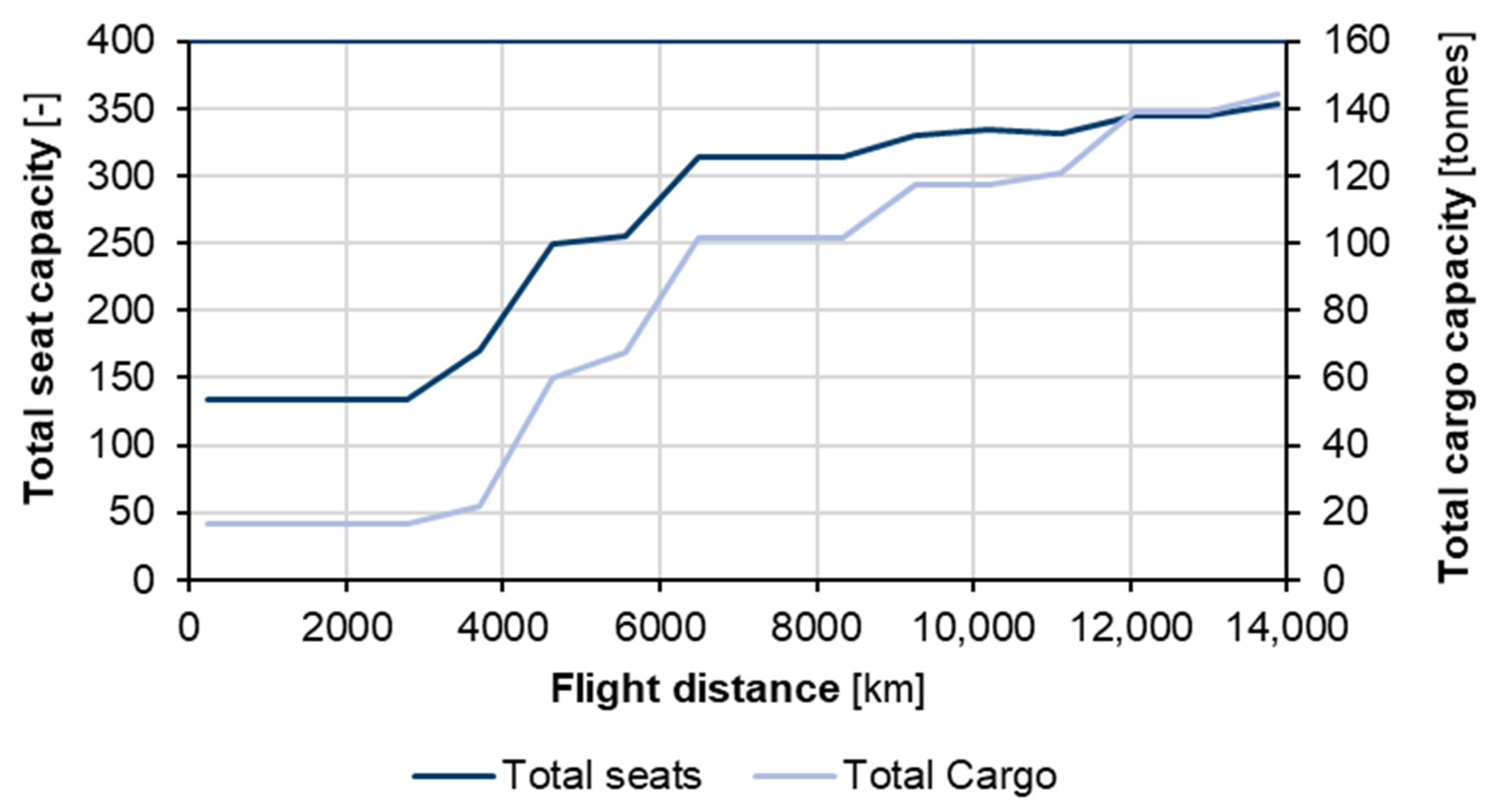
In this section, the data used to build the non-road vehicle models are outlined. The future development scenarios are also justified.

4.2.1. Airplanes

Due to the complex physics entailed by airplane flight, a different approach is considered for the aviation fuel demand model. First, the German aviation sector must be better understood. The Lufthansa Group has the largest market share, at 87.1% as of 2018 [63], of the national industry and the second-largest in Europe [64]. In addition to the airplanes of the Lufthansa Group’s fleet, other widely used models in the industry are also considered to increase the robustness of the fuel demand results.

The impact of flight distances on fuel consumption is considered by using the Aviation Emissions Calculator (AEC) accompanying the EMEP/EEA air pollutant emission inventory guidebook. The fuel demand is thereby determined for the selected airplane models and for different flight distances [65]. Figure 7 shows the total seating and cargo capacity as a function of the flight distance incorporated in the model.

For each discrete flight distance, multiple possible airplane models are chosen. Future improvement in energy demand per decade is approximately 10% [26].

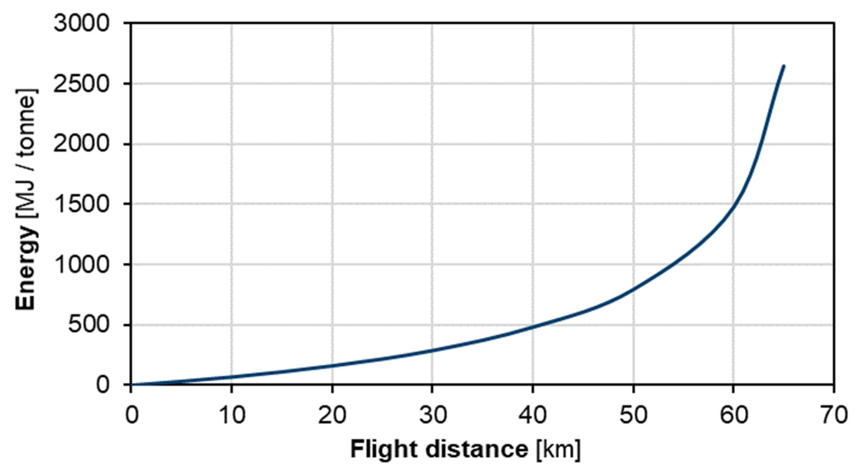
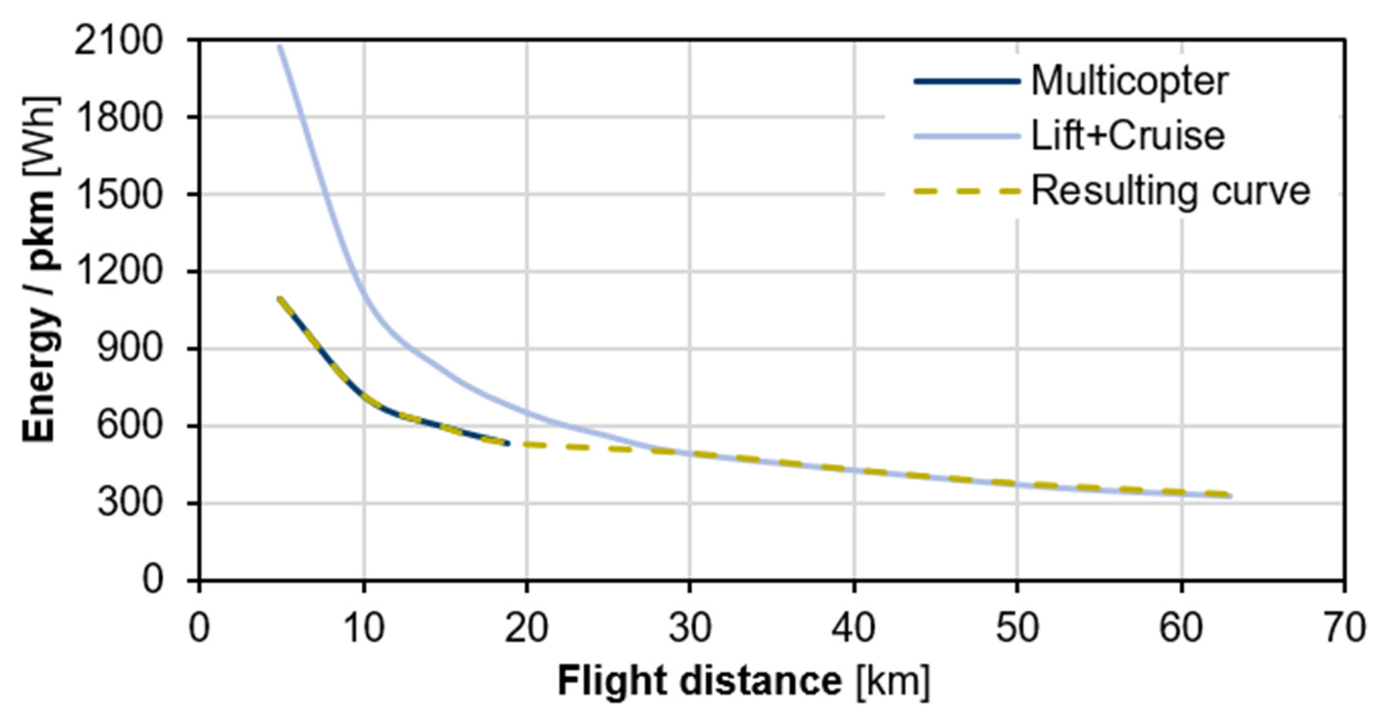
4.2.2. Unmanned Aviation

Xu (2017) models the energy demand of differently sized freight unmanned aviation. Figure 8 displays the energy demand for delivery as a function of the flight distance [27].

Bauhaus Luftfahrt reports on the energy demand for the two major passenger unmanned aviation configurations, namely multicopter and lift+cruise. The results indicate that multicopter unmanned aviation requires less energy, although their flight range is limited compared to lift+cruise models. Figure 9 shows the energy demand per passenger-kilometer for different flight distances for unmanned aviation with a maximum capacity of four passengers [28].

Figure 9 also reveals the resulting curve used to model the energy demand for passenger unmanned aviation.

4.2.3. Trains

Trains are an important mode of transportation. Rail transport was responsible for 4.5% of the sector’s total carbon emissions for the year 2014 in Germany [66]. The railway model is based on data in the literature and considers four different modes: trams, short- and long-distance trains, and freight trains.

With respect to trams, Kuminek reports the energy consumption values for electric catenary trams [67]. Energy demand for electric and diesel short-distance trains and freight trains can be found in the Global Emissions Model for Integrated Systems (GEMIS) database [68]. The data on long-distance trains are drawn from Deutsche Bahn’s Integrated Report [69]. The FCEV freight train data are based on Bründlinger et al. [70].

4.2.4. Ships

The importance of ships in global freight transport cannot be understated. Shipping accounts for approximately 75% of global freight transportation, and it is the most energy-efficient means of carrying cargo [71].

As with trains and aviation models, the shipping model is based on data from the literature. The energy demand for international shipping is derived from the IEA [71], whereas that for national shipping (inland waterway transport) is based on Bründlinger et al. [70].

4.3. Occupancy and Loading Rates

The occupancy and loading rates for the various transport modes are taken from the literature.

Table 3. Default occupancy rates for the different modes [52,69,72,73,74].

Mode	Occupancy/Loading Rate [%]	Sources
LDV	26	[52]
Bus	19	[72]
Coach	57	[72]
Small truck	32	[72]
Medium truck	32	[72]
Large truck	35	[72]
Semi-truck	45	[72]
Airplane	82	[73]
Drone	82	-
Tram	18	[74]
Short-distance train	21	[74]
Long-distance train	56	[69]
Freight train	38	[74]
National shipping	50	[72]
International shipping	80	-

shows the default occupancy and loading rates for all transport modes used in the model.

5. Results and Discussion

The results obtained from the developed model are discussed in this section. First, the effects of varying vehicle parameters are analyzed for different driving conditions in Section 5.1. A modal analysis was carried out for both passenger and freight transport modes. Next, the energy consumption of different drivetrains for medium cars is analyzed. The effects of electrification on the energy demand of a vehicle are then discussed. Next, the effects of the driving environment on the energy demand for trucks and buses are assessed. The section concludes with a comparison of the results from the model with those from other studies.

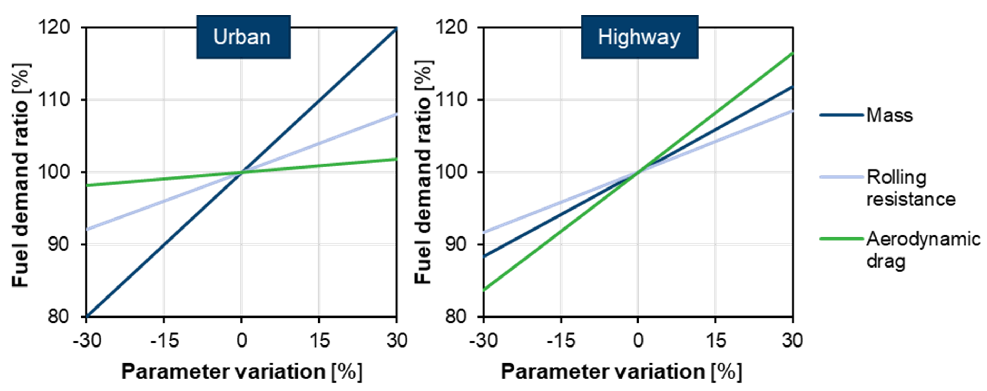
5.1. Parameter Variation

In this section, the effects of changing a vehicle’s mass, aerodynamic properties, and rolling resistance on a medium-sized BEV’s fuel energy demand are evaluated. The effects were analyzed for urban and highway driving conditions and are shown in Figure 10.

The left panel of Figure 10 shows that reducing the vehicle mass has the largest effect on urban driving conditions due to the stop-and-go driving style prevalent in urban conditions. A 10% reduction in vehicle mass resulted in a 6.7% lower fuel energy demand. If the vehicle did not have regenerative braking, the effects would be more pronounced. Changing the aerodynamic drag had the lowest impact on the final energy demand due to the low average speed in urban conditions. The aerodynamic drag force is proportional to the square of the vehicle’s velocity.

The right panel of Figure 10 shows that changing the aerodynamic drag had the highest impact on the energy demand for highway driving conditions due to the higher speeds of highway driving, which results in a higher proportion of the total energy demand being used to overcome aerodynamic drag. A 10% improvement in vehicle aerodynamics reduced energy consumption by 5.5%. Meanwhile, variation in rolling resistance has the lowest impact on vehicle energy demand for highway driving conditions.

5.2. Modal Analysis

This section discusses the fuel energy demand for conventional, hydrogen, and electric drivetrains among the different modes. The discussion is further divided into passenger and freight modes.

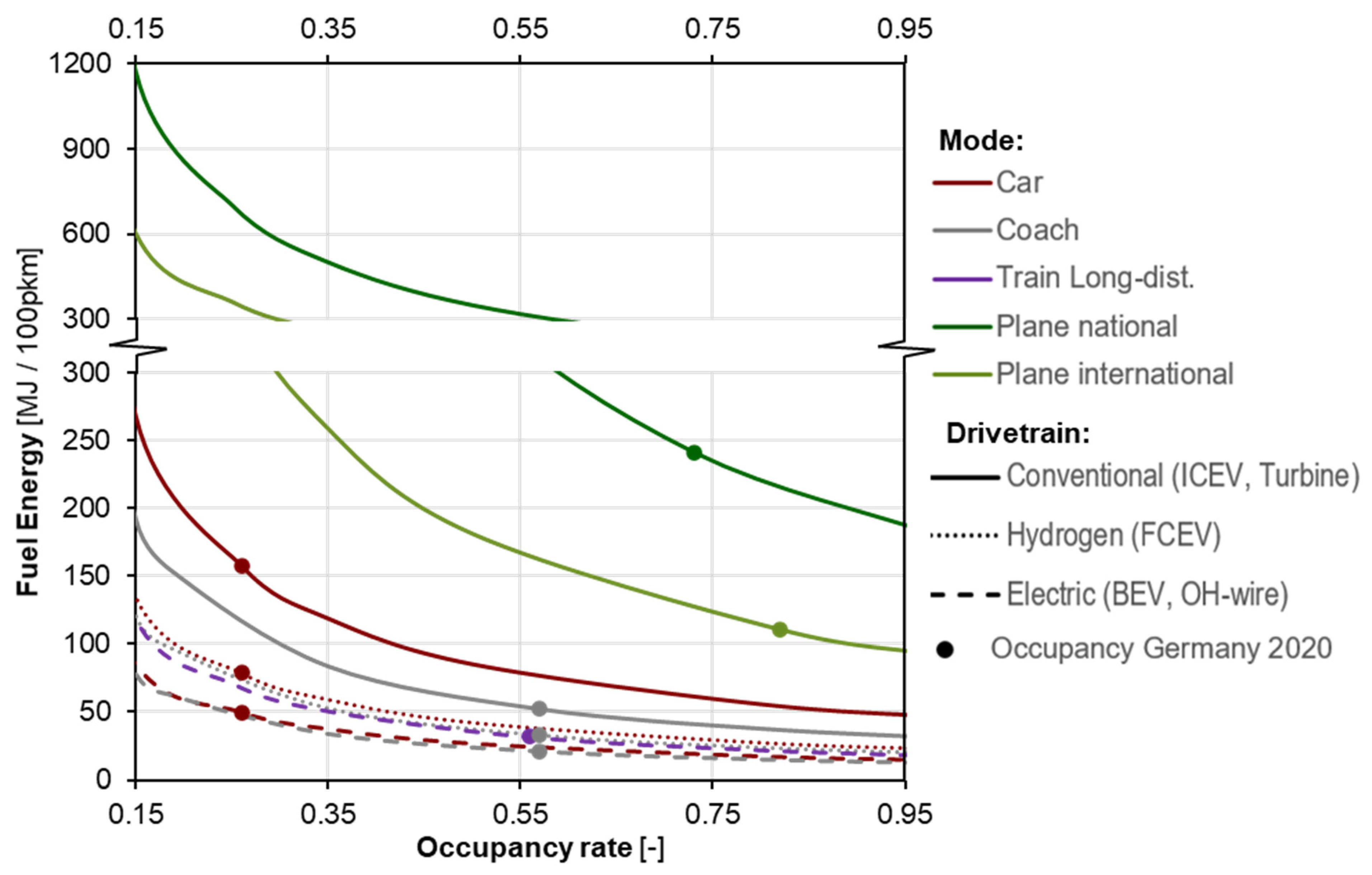
5.2.1. Passenger Modes

Figure 11 shows the fuel demand for selected short-distance passenger transport modes in terms of energy per 100 passenger-kilometers (pkm) for varying occupancy rates. The default occupancy rates for 2020 are highlighted for each drivetrain [72].

As is shown in Figure 11, unmanned aviation features the highest energy consumption for short-distance passenger transport, 217 MJ/100 pkm for the average occupancy rate.

After unmanned aviation, ICEV-g medium cars (158 MJ/100 pkm) feature the highest energy consumption rates for all occupancies. In contrast, battery electric cars and buses, fuel cell buses, and trams have some of the lowest, at 50, 34, 52, and 43 MJ/100 pkm, respectively, at average occupancy for Germany in the year 2020.

Overall, Figure 11 clearly shows the effects of occupancy rates on fuel demand per 100 pkm. The exponential rise in energy demand for low occupancy rates underlines the importance of high occupancy rates on reducing the overall transport sector energy demand while still maintaining passenger capacity.

Figure 12 displays the fuel demand for select long-distance passenger transport modes in terms of energy per 100 pkm, for varying occupancy rates. The default occupancy rates for 2020 are highlighted for each drivetrain [72].

Figure 12 shows that airplanes have the highest energy demand among all occupancy rates, with national flights yielding the highest values (241 MJ/100 pkm).

After airplanes, ICEV-g medium cars (158 MJ/100 pkm) have the highest energy consumption for all occupancies, whereas BEV and FCEV coaches and long-distance trains have the least, at 21, 33, and 32 MJ/100 pkm, respectively.

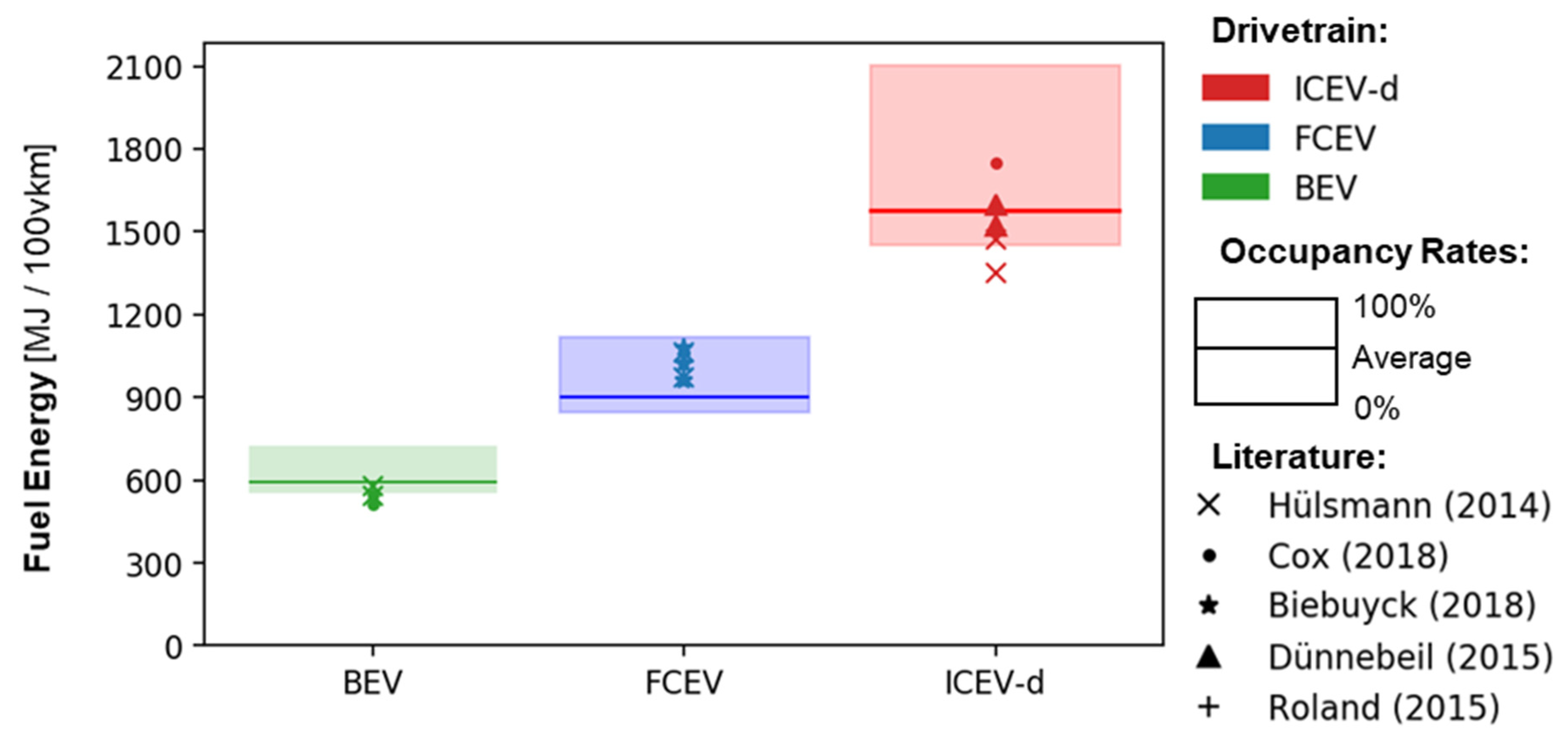
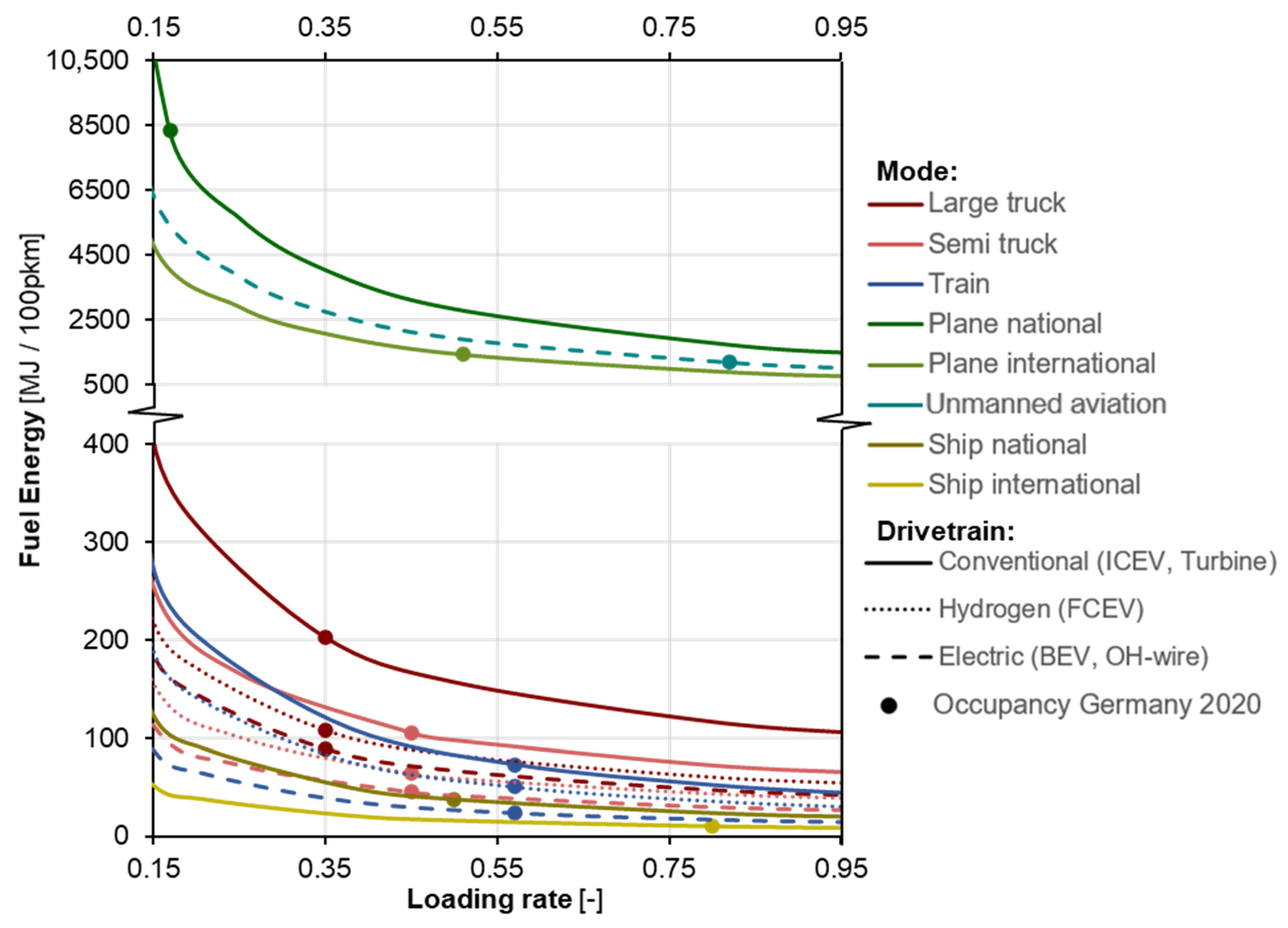
5.2.2. Freight Modes

Figure 13 displays the fuel demand for select freight transport modes in terms of energy per 100 tonne-kilometer (tkm) transported for varying loading rates. The default loading rates for 2020 are highlighted for each drivetrain [72].

Figure 13 shows that the aviation modes have the worst energy consumption of all freight transport modes, of between 1174 and 8327 MJ/100 tkm for the average loading rates. Unmanned aviation features the additional benefit of fulfilling door-to-door transport needs.

Figure 13 also shows that fuel energy depends on the different modes’ loading rates. After the aviation modes, ICEV-d large trucks (203 MJ/100 tkm) have the worst energy consumption values, whereas international shipping has the best (9.9 MJ/100 tkm). National shipping is also one of the most energy-efficient modes, although the availability of accessible inland water bodies must be considered. Electric freight trains (23 MJ/100 tkm) and BEV semi-trucks (45 MJ/100 tkm) offer the best solutions for on-land freight transportation.

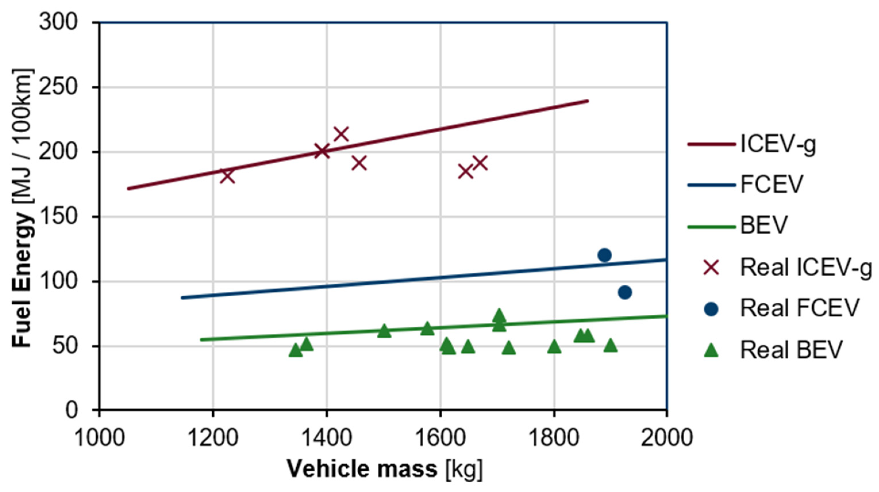
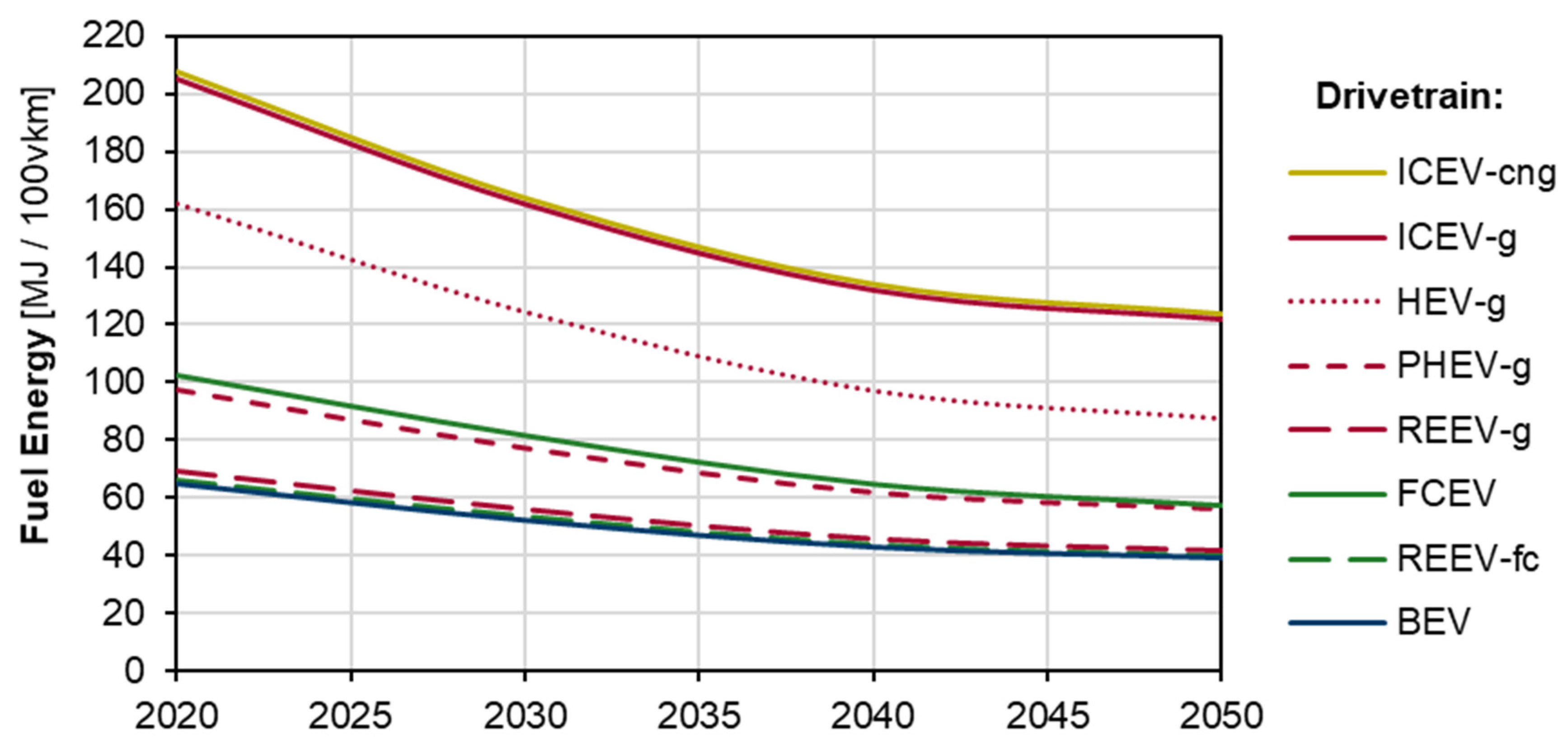
5.3. Drivetrain Analysis

In this section, the energy demands for the different drivetrains of medium cars are presented. The energy demand for the different drivetrains through 2050 is shown in Figure 14 in terms of energy per 100 vehicle-kilometers (vkm).

Figure 14 shows that, of all of the different drivetrains, ICEVs have the highest energy demand. HEV-g exhibits lower energy consumption values due to having better drivetrain efficiencies and the use of regenerative braking. PHEV-g and REEV-g show lower energy consumption values due to the all-electric driving option. BEVs have the lowest energy consumption values.

Furthermore, the HEV-g exhibits the most significant relative improvement of 45.7% through 2050, whereas BEVs show, with 39.6%, the least. In terms of energy demand, the ICEV-cng and ICEV-g both reduce their energy demand by roughly 80 MJ/100 vkm to reach around 120 MJ/100 vkm by 2050. The fuel energy demand decreases more slowly between 2040 and 2050 because of the lower efficiency gain in this timeframe compared to the period 2020–2040 (cf. Table 2).

5.4. Electric Share

In this section, the change in fuel energy demand in accordance with increased drivetrain electrification is analyzed. An HEV-g medium car is considered for a vehicle with a 0% electric drive share, whereas a BEV represents a vehicle with a 100% electric share. A PHEV-g car is used to model electric drive shares in between. Figure 15 displays the results of this analysis.

Figure 15 shows how the fuel energy demand drastically decreases with the increase in the electric share. A drivetrain with a 100% electric share has almost 60% lower fuel demand than a drivetrain with a 0% electric share. It is assumed that a PHEV has the same configuration (battery capacity) and, therefore, the same vehicle mass. Only user behavior leads to different electric shares.

5.5. Effects of the Driving Environment

In this section, the effects of the driving environment on the fuel energy demand of different trucks and medium buses are discussed.

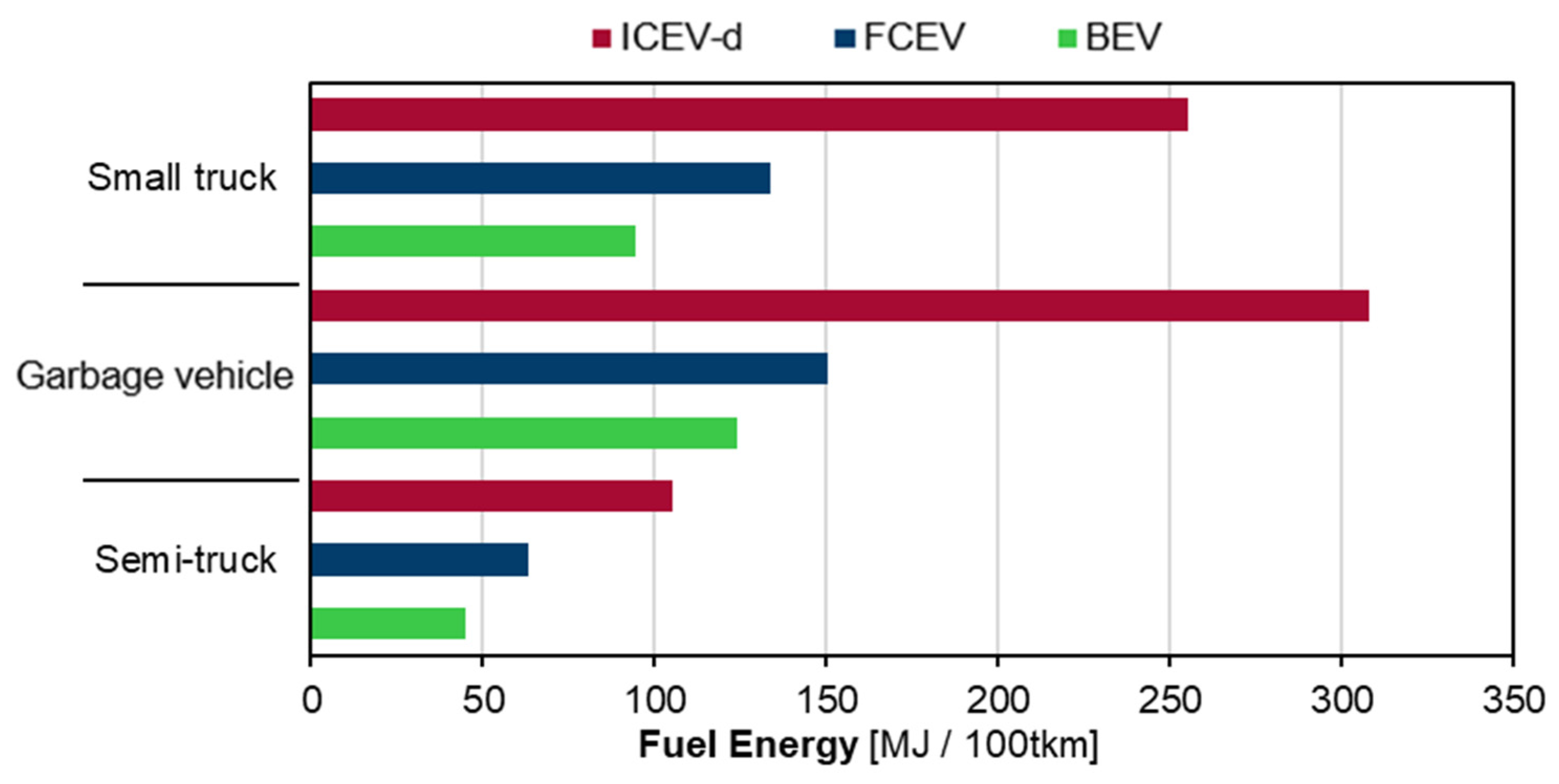
5.5.1. Trucks for Different Purposes

In this section, the energy demands for the trucks used for different functions are first analyzed. A small truck used for urban cargo delivery is evaluated using the urban and rural parts of the World Harmonized Vehicle Cycle (WHVC) [75]. A large truck used for urban waste collection is assessed using the Neighborhood Refuse Truck Cycle [76]. Finally, a semi-truck used for long-haul freight transportation is considered using the highway segment of the WHVC. Default loading rates are assumed for all modes. Figure 16 displays the results obtained from this analysis.

Figure 16 shows that urban waste collection is the most energy-intensive, whereas long-haul freight transport is the least energy-intensive for all drivetrains. Urban cargo and waste collection benefit the most from drivetrain electrification, with roughly a 60% drop in fuel energy demand. This is due to the prevalence of stop-and-go driving conditions for these vehicles. Long-haul cargo is the least energy-intensive due to the vehicles’ higher loading rates and the lack of stops, which significantly impact the trucks’ energy demand due to their large masses.

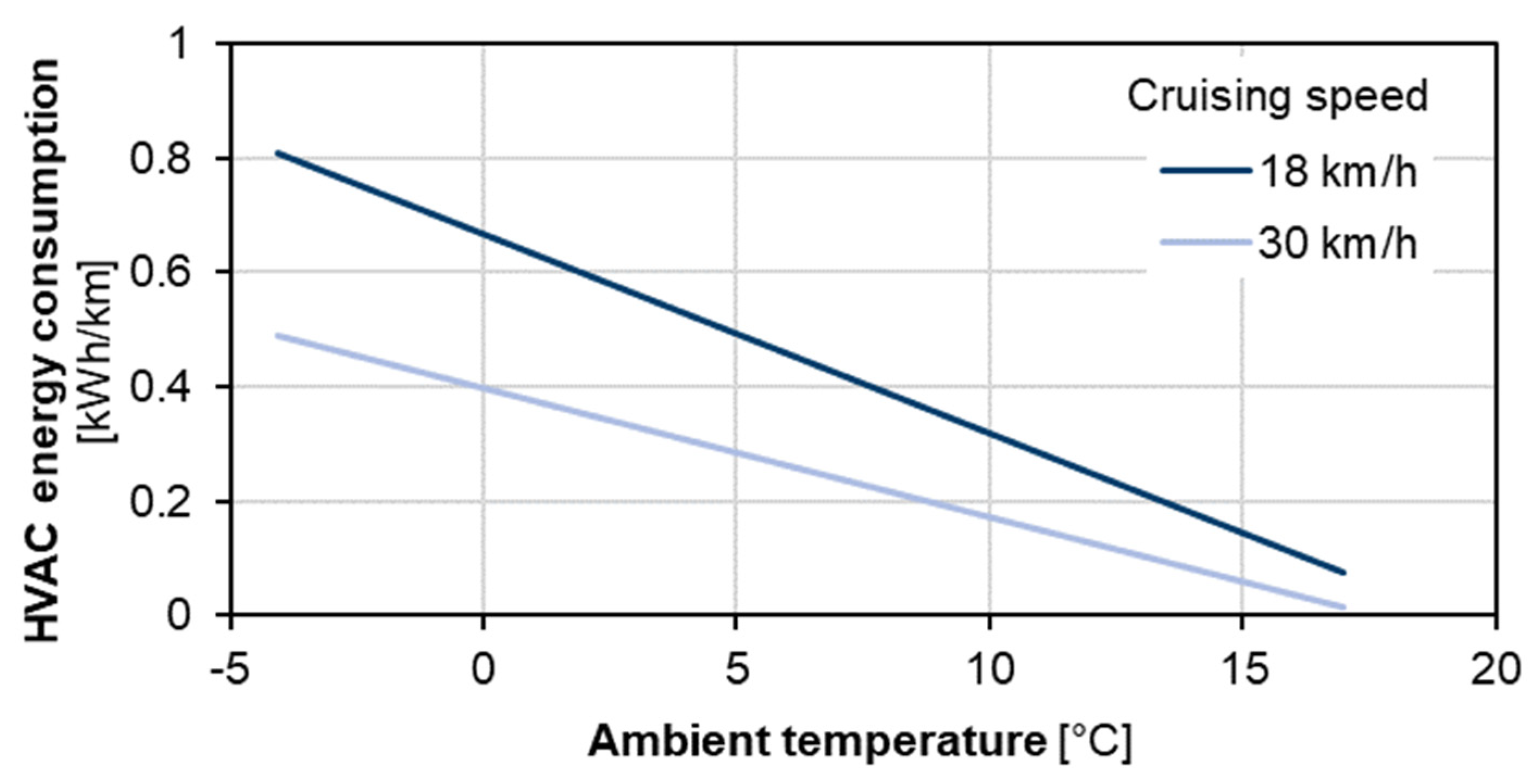
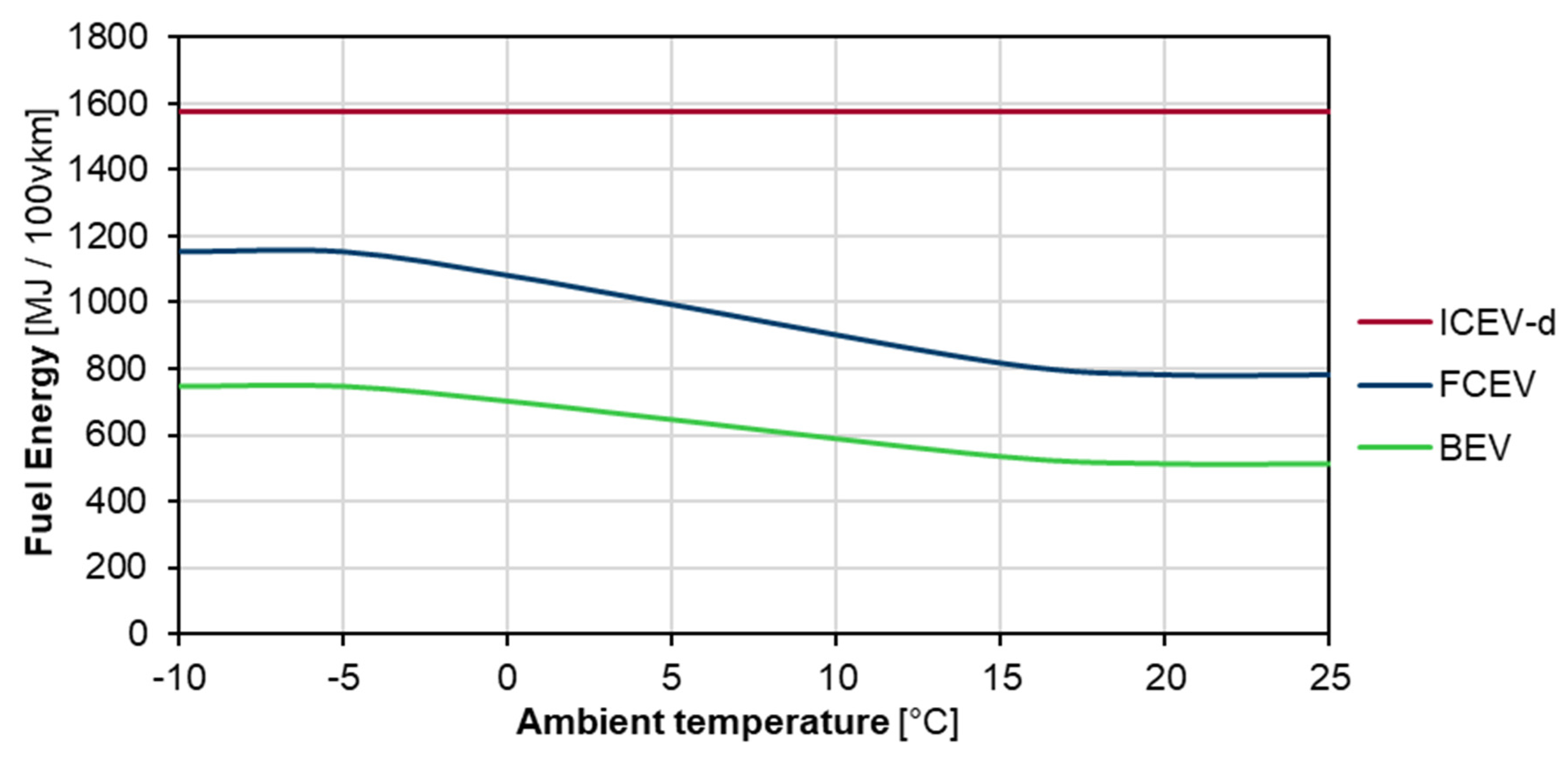
5.5.2. Effects of Ambient Temperature on Buses

The impact of ambient temperature variations on the fuel energy demand for a medium bus is analyzed next, over a temperature range of −10 to 25 °C, as depicted in Figure 17. Only the energy demand for heating and ventilation is considered.

Figure 17 shows that the energy demand for ICEV-d does not change with temperature variations, assuming that the engine’s waste heat meets the thermal energy requirements. For FCEVs and BEVs, the energy demand depends on ambient temperatures of between approximately −5 and 17 °C. It is assumed that the vehicle only needs to use ventilation at higher temperatures; for lower temperatures, it is assumed that the vehicle’s heating capacity is reached. Moving from a temperature of 20 °C to −5 °C, the fuel energy demand for the BEV increases by almost 50%, rising from 511.0 to 745.8 MJ/100 vkm, whereas the ICEV-d energy consumption remains constant at 1572.8 MJ/100 vkm.

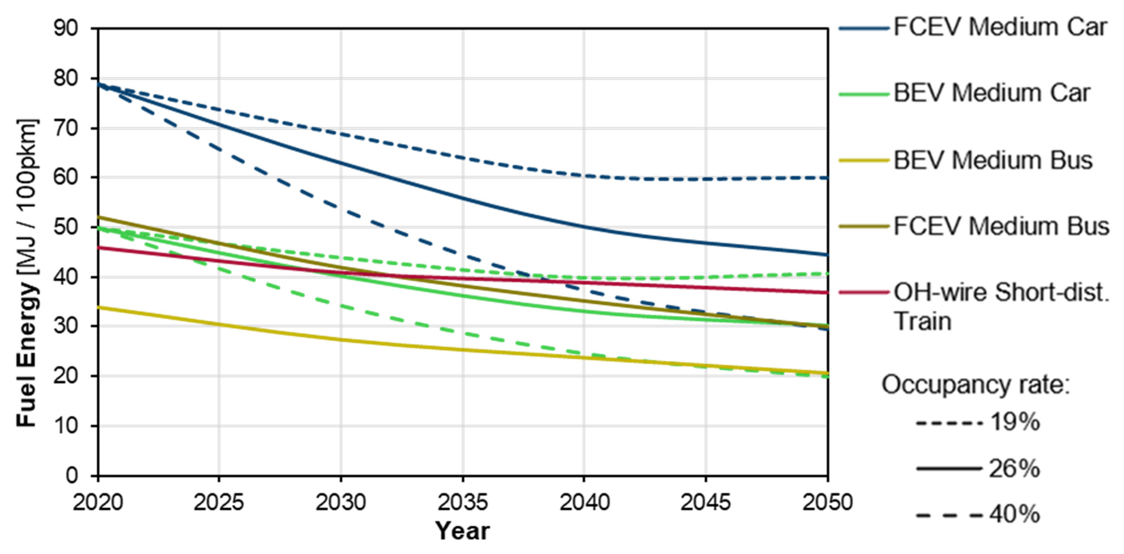
5.6. Change in Occupancy through 2050

The effects of increased autonomous driving on occupancy rates and fuel energy demand are discussed in this section. Harb et al. (2018) assessed the effects of occupancy rates and vehicle miles traveled by providing 13 subjects with chauffeur services for a week. The study found that the vehicle miles traveled tended to increase as the subjects sent their vehicles for errands. These trips would equate to a 0% occupancy rate trip for autonomous vehicles [77]. This indicates that the average occupancy rates are lower for private vehicles with the emergence of accessible autonomous driving.

On the other hand, autonomous driving could facilitate increased ridesharing. The effects of shared self-driving urban mobility in the city of Lisbon, Portugal were modeled by Martinez and Viegas, the results of which showed that the occupancy rates of these shared vehicles could be between 40% and 60% [78]. Raposo et al. (2018) report that the occupancy rates can vary between 19% and 40%, depending on how many of the trips are shared [79].

Taking the occupancy rates reported in Raposo et al. (2018) to be for the year 2050, the effects of changes in occupancy rates on the fuel energy demand per passenger in a medium car are depicted in Figure 18. It is estimated that the occupancy rates will change linearly from 2020 through 2050. The figure also indicates the energy demand for a constant occupancy rate of 26% for the car. BEVs and FCEVs were chosen for this analysis based on their anticipated future importance. The energy demand for battery electric and fuel cell medium buses and an electric short-distance train are also represented for comparison. The occupancy rates for the buses and trains are assumed to be constant at 19% and 27%, respectively [72], over the timefame.

Figure 18 highlights the importance of future user behavior for reducing the energy demand per pkm. User behavior, which changes the average occupancy rate, can vary the energy demand from 20.0 to 40.8 MJ/100 pkm for BEVs, and from 29.4 to 60.1 MJ/100 pkm for FCEVs by 2050. For the higher occupancy rates, the energy demand for a BEV car can be better than that for a battery electric bus in 2050, assuming that the occupancy rates for buses do not significantly change.

6. Conclusions

The German transport sector is currently in the midst of undergoing a massive transformation as part of the country’s attempt to meet its climate targets. It is expected that there will be profound modal shifts in the transport sector. This paper aims to build a tank-to-wheel energy model for the major modes of transport in Germany. Furthermore, future efficiency improvements were also considered for the various modes. The results were validated through a comparison with data reported for real vehicles and those from the literature.

Driving conditions were the most important criterion when comparing the vehicle energy demand across drivetrains. On the other hand, occupancy rates were the most critical indicator when comparing energy demand between the different modes.

For both short- and long-distance passenger transport, public transportation was often found to be the most energy-efficient means. For short-distance journeys, battery electric buses (33.9 MJ/100 pkm) and trams (45.8 MJ/100 pkm), and for long-distance journeys, battery electric coaches (21.3 MJ/100 pkm) and electric trains (31.8 MJ/100 pkm), represented the highest energy efficiencies. The aviation modes considered in this model generally featured the highest energy consumption, at between 110 and 217 MJ/100 pkm.

With respect to freight transportation, international shipping (9.9 MJ/100 tkm) was the most energy-efficient, whereas national flights (1726 MJ/100 tkm) exhibited the lowest energy efficiency. For national freight transport, electric trains (35.2 MJ/100 tkm), as well as battery electric (45.1 MJ/100 tkm) and fuel cell (64.2 MJ/100 tkm) semi-trucks, represented some of the best modes.

In future transport, the first aim should be to increase occupancy rates. This will be challenging to implement, but it is a free upgrade, as no additional technology investment is required to decrease the energy intensity of transport. Furthermore, the increased electrification of drivetrains will reduce the final energy demand for the transport sector.

References

1. IPBES. Summary for Policymakers of the Ipbes Global Assessment Report on Biodiversity and Ecosystem Services. 2019. Available online: https://ipbes.net/system/tdf/ipbes_global_assessment_report_summary_for_policymakers.pdf?file=1&type=node&id=35329 (accessed on 18 January 2022).
2. Indicator: Greenhouse Gas Emissions|Umweltbundesamt. Available online: https://www.umweltbundesamt.de/en/indicator-greenhouse-gas-emissions#at-a-glance (accessed on 1 February 2021).
3. Climate Change Act—Climate Neutrality by 2045. Available online: https://www.bundesregierung.de/breg-de/themen/klimaschutz/climate-change-act-2021-1913970 (accessed on 17 October 2021).
4. Climate Action Plan 2050—Germany’s Long-Term Emission Development Strategy|BMU. The Federal Minister for the Environment, Nature Conservation, and Nuclear Safety; Available online: https://www.bmu.de/en/topics/climate-energy/climate/national-climate-policy/greenhouse-gas-neutral-germany-2050/ (accessed on 5 July 2020).
5. Amelang, S. Germany commits additional €3 bln to ease green mobility transition in car industry. Clean Energy Wire 2020. Available online: https://www.cleanenergywire.org/news/germany-commits-additional-eu3-bln-ease-green-mobility-transition-car-industry (accessed on 14 December 2020).
6. Jardin, P.; Esser, A.; Givone, S.; Eichenlaub, T.; Schleiffer, J.-E.; Rinderknecht, S. The Sensitivity in Consumption of Different Vehicle Drivetrain Concepts Under Varying Operating Conditions: A Simulative Data Driven Approach. Vehicles 2019, 1, 69–87. [Google Scholar] [CrossRef] [Green Version]
7. Gao, D.W.; Mi, C.; Emadi, A. Modeling and Simulation of Electric and Hybrid Vehicles. Proc. IEEE 2007, 95, 729–745. [Google Scholar] [CrossRef]
8. Fiori, C.; Ahn, K.; Rakha, H.A. Power-based electric vehicle energy consumption model: Model development and validation. Appl. Energy 2016, 168, 257–268. [Google Scholar] [CrossRef]
9. Halbach, S.; Sharer, P.; Pagerit, S.; Rousseau, A.P.; Folkerts, C. Model architecture, methods, and interfaces for efficient math-based design and simulation of automotive control systems. SAE Tech. Pap. 2010, 2010, 20100241. [Google Scholar] [CrossRef] [Green Version]
10. Ahmad, F.; Mazlan, S.A.; Zamzuri, H.; Jamaluddin, H.; Hudha, K.; Short, M. Modelling and validation of the vehicle longitudinal model. Int. J. Automot. Mech. Eng. 2014, 10, 2042–2056. [Google Scholar] [CrossRef]
11. Edwardes, W.; Rakha, H. Virginia tech comprehensive power-based fuel consumption model. Transp. Res. Rec. 2014, 2428, 1–9. [Google Scholar] [CrossRef]
12. Edwardes, W.; Rakha, H. Modeling diesel and hybrid bus fuel consumption with Virginia Tech comprehensive power-based fuel consumption model: Model enhancements and calibration issues. Transp. Res. Rec. 2015, 2533, 100–108. [Google Scholar] [CrossRef]
13. Park, S.; Rakha, H.; Ahn, K.; Moran, K. Virginia Tech Comprehensive Power-based Fuel Consumption Model (VT-CPFM): Model Validation and Calibration Considerations. Int. J. Transp. Sci. Technol. 2013, 2, 317–336. [Google Scholar] [CrossRef] [Green Version]
14. Vagg, C.; Brace, C.J.; Akehurst, S.; Ash, L. Minimizing battery stress during hybrid electric vehicle control design: Real world considerations for model-based control development. In Proceedings of the 2013 9th IEEE Vehicle Power and Propulsion Conference IEEE VPPC 2013, Beijing, China, 15–18 October 2013; pp. 329–334. [Google Scholar] [CrossRef] [Green Version]
15. Abousleiman, R.; Rawashdeh, O. Energy consumption model of an electric vehicle. In Proceedings of the 2015 IEEE Transportation Electrification Conference and Expo, ITEC 2015, Dearborn, MI, USA, 14–17 June 2015. [Google Scholar] [CrossRef]
16. Luin, B.; Petelin, S.; Al-Mansour, F. Microsimulation of electric vehicle energy consumption. Energy 2019, 174, 24–32. [Google Scholar] [CrossRef]
17. Hayes, J.G.; Davis, K. Simplified electric vehicle powertrain model for range and energy consumption based on EPA Coast-down Parameters and Test Validation by Argonne national lab data on the Nissan leaf. In Proceedings of the 2014 IEEE Transportation Electrification Conference and Expo Components, System Power Electron—From Technology to Bussiness Public Policy, ITEC 2014, Dearborn, MI, USA, 16–19 June 2014; Available online: https://ieeexplore.ieee.org/document/6861831 (accessed on 18 January 2022).
18. Grube, T.; Stolten, D. The impact of drive cycles and auxiliary power on passenger car fuel economy. Energies 2018, 11, 1010. [Google Scholar] [CrossRef] [Green Version]
19. Bielaczyc, P.; Szczotka, A.; Woodburn, J. The effect of a low ambient temperature on the cold-start emissions and fuel consumption of passenger cars. Proc. Inst. Mech. Eng. Part D J. Automob. Eng. 2011, 225, 1253–1264. [Google Scholar] [CrossRef]
20. Duarte, G.O.; Gonçalves, G.A.; Farias, T.L. Analysis of fuel consumption and pollutant emissions of regulated and alternative driving cycles based on real-world measurements. Transp. Res. Part D Transp. Environ. 2016, 44, 43–54. [Google Scholar] [CrossRef]
21. Energy Statistics—An Overview Statistics Explained. Available online: https://ec.europa.eu/eurostat/statisticsexplained/ (accessed on 15 October 2020).
22. Teter, J.; Le Feuvre, P.; Bains, P.; Re, L. IEA. Aviation, IEA, Paris. 2020. Available online: https://www.iea.org/reports/aviation (accessed on 14 February 2021).
23. Burzlaff, M. Aircraft Fuel Consumption—Estimation and Visualization. Fuel Consum. 2017. [Google Scholar] [CrossRef]
24. Park, Y.; O’Kelly, M.E. Fuel burn rates of commercial passenger aircraft: Variations by seat configuration and stage distance. J. Transp. Geogr. 2014, 41, 137–147. [Google Scholar] [CrossRef]
25. Peeters, P.; Middel, J.; Hoolhorts, A. Fuel Efficiency of Commercial Aircraft: An Overview of Historical and Future Trends; National Aerospace Laboratory NLR: Amsterdam, The Netherlands, 2005; Available online: https://www.transportenvironment.org/sites/te/files/media/2005-12_nlr_aviation_fuel_efficiency.pdf (accessed on 18 January 2022).
26. Kharina, A.; Rutherford, D. Fuel Efficiency Trends for New Commercial Jet Aircraft: 1960 to 2014; The International Council on Clean Transportation: Washington, DC, USA, 2015; Available online: https://theicct.org/wp-content/uploads/2021/06/ICCT_Aircraft-FE-Trends_20150902.pdf (accessed on 18 January 2022).
27. Xu, J. Design Perspectives on Delivery Drones; RAND Corporation: Santa Monica, CA, USA, 2017. [Google Scholar] [CrossRef] [Green Version]
28. Electric VTOL Aircraft for Urban Air Mobility: Bauhaus Luftfahrt. Available online: https://www.bauhaus-luftfahrt.net/en/research/systems-aircraft-technologies/electric-vtol-aircraft-for-urban-air-mobility/ (accessed on 28 September 2020).
29. Zhang, H.; Jia, L.; Wang, L.; Xu, X. Energy consumption optimization of train operation for railway systems: Algorithm development and real-world case study. J. Clean. Prod. 2019, 214, 1024–1037. [Google Scholar] [CrossRef]
30. Salvador, P.; Martínez, P.; Villalba, I.; Insa, R. Modelling energy consumption in diesel multiple units. Proc. Inst. Mech. Eng. Part F J. Rail Rapid Transit 2018, 232, 1539–1548. [Google Scholar] [CrossRef]
31. Wang, J.; Rakha, H.A. Electric train energy consumption modeling. Appl. Energy 2017, 193, 346–355. [Google Scholar] [CrossRef] [Green Version]
32. Kee, K.-K.; Lau Simon, B.-Y.; Yong Renco, K.-H. Prediction of Ship Fuel Consumption and Speed Curve by Using Statistical Method. J. Comput. Sci. Comput. Math. 2018, 8, 19–24. [Google Scholar] [CrossRef] [Green Version]
33. Jeon, M.; Noh, Y.; Shin, Y.; Lim, O.-K.; Lee, I.; Cho, D. Prediction of ship fuel consumption by using an artificial neural network. J. Mech. Sci. Technol. 2018, 32, 5785–5796. [Google Scholar] [CrossRef]
34. Yang, L.; Chen, G.; Rytter, N.G.M.; Zhao, J.; Yang, D. A genetic algorithm-based grey-box model for ship fuel consumption prediction towards sustainable shipping. Ann. Oper. Res. 2019, 813, 13. [Google Scholar] [CrossRef]
35. Germany—Countries & Regions—IEA. Available online: https://www.iea.org/countries/germany (accessed on 9 July 2020).
36. Guzzella, L.; Sciarretta, A. Vehicle Propulsion Systems, 2nd ed.; Springer: Zürich, Switzerland, 2007; ISBN 9783540746911. [Google Scholar]
37. Grube, T. Potentiale des Strommanagements zur Reduzierung des Spezifischen Energiebedarfs von Pkw; Technische Universität: Berlin, Germany, 2014. [Google Scholar]
38. National Research Council of the National Academies. Transitions to Alternative Vehicles and Fuels; National Research Council of the National Academies: Washington, DC, USA, 2013. Available online: https://www.nap.edu/catalog/18264/transitions-to-alternative-vehicles-and-fuels (accessed on 18 January 2022). [CrossRef]
39. Rajamani, R. Vehicle Dynamics and Control, 1st ed.; Ling, F.F., Ed.; Springer: Berlin/Heidelberg, Germany, 2006; ISBN 9780387263960. [Google Scholar]
40. Forward and Backward Euler Methods. Available online: https://web.mit.edu/10.001/Web/Course_Notes/Differential_Equations_Notes/node3.html (accessed on 16 September 2020).
41. Barlow, T.J.; Latham, S.; Mccrae, I.S.; Boulter, P.G. A Reference Book of Driving Cycles for Use in the Measurement of Road Vehicle Emissions; Berkshire; 2009; Available online: https://trid.trb.org/view/909274 (accessed on 18 January 2022).
42. Emission Test Cycles: WLTC. Available online: https://dieselnet.com/standards/cycles/wltp.php (accessed on 10 July 2020).
43. Office for Official Publications of the European Communities L-2985 Luxembourg. Regulation (EEC) No 4064/89 Merger Procedure Article 6(1)(b); Office for Official Publications of the European Communities L-2985 Luxembourg: Brussels, Belgium, 1999. [Google Scholar]
44. Islam, E.S.; Moawad, A.; Kim, N.; Rousseau, A. Energy Consumption and Cost Reduction of Future Light-Duty Vehicles through Advanced Vehicle Technologies: A Modeling Simulation Study Through 2050; Argonne National Lab.: Argonne, IL, USA, 2020. Available online: https://publications.anl.gov/anlpubs/2020/08/161542.pdf (accessed on 18 January 2022).
45. Al-Samari, A. Study of emissions and fuel economy for parallel hybrid versus conventional vehicles on real world and standard driving cycles. Alex. Eng. J. 2017, 56, 721–726. [Google Scholar] [CrossRef]
46. Spanoudakis, P.; Tsourveloudis, N.; Doitsidis, L.; Karapidakis, E. Experimental Research of Transmissions on Electric Vehicles’ Energy Consumption. Energies 2019, 12, 388. [Google Scholar] [CrossRef] [Green Version]
47. Drivetrain Losses (Efficiency)—x-engineer.org. Available online: https://x-engineer.org/automotive-engineering/drivetrain/transmissions/drivetrain-losses-efficiency/ (accessed on 17 September 2020).
48. Li, K.; Tseng, K.J. Energy efficiency of lithium-ion battery used as energy storage devices in micro-grid. In Proceedings of the IECON 2015—41st Annual Conference of the IEEE Industrial Electronics Society, Yokohama, Japan, 9–12 November 2015; Institute of Electrical and Electronics Engineers Inc.: Piscataway, NJ, USA, 2015; pp. 5235–5240. [Google Scholar]
49. Schimpe, M.; Naumann, M.; Truong, N.; Hesse, H.C.; Santhanagopalan, S.; Saxon, A.; Jossen, A. Energy efficiency evaluation of a stationary lithium-ion battery container storage system via electro-thermal modeling and detailed component analysis. Appl. Energy 2018, 210, 211–229. [Google Scholar] [CrossRef]
50. Eftekhari, A. Energy efficiency: A critically important but neglected factor in battery research. Sustain. Energy Fuels 2017, 1, 2053–2060. [Google Scholar] [CrossRef]
51. Trost, T. Erneuerbare Mobilität im Motorisierten Individualverkehr; Fraunhofer Verlag: Stuttgart, Germany, 2017; ISBN 9783839611296. [Google Scholar]
52. Occupancy Rates—European Environment Agency. Available online: https://www.eea.europa.eu/publications/ENVISSUENo12/page029.html (accessed on 15 October 2020).
53. Air—Density, Specific Weight and Thermal Expansion Coefficient at Varying Temperature and Constant Pressures. Available online: https://www.engineeringtoolbox.com/air-density-specific-weight-d_600.html?vA=15&units=C# (accessed on 17 September 2020).
54. Berdowski, Z.; Broek-Serlé, F.N.; Jetten, J.T.; Kawabatta, Y.; Schoemaker, J.T.; Versteegh, R. Survey on Standard Weights of Passengers and Baggage Final Report. Available online: https://www.easa.europa.eu/system/files/dfu/WeightSurveyR20090095Final.pdf (accessed on 18 January 2022).
55. Cox, B. Mobility and the Energy Transition: A Life Cycle Assessment of Swiss Passenger Transport Technologies Including Developments Until 2050. Ph.D. Thesis, ETH Zurich, Zurich, Switzerland, 2018. [Google Scholar] [CrossRef]
56. Knote, T.; Haufe, B.; Saroch, L. Gefördert durch das Bundesministerium für Umwelt, Naturschutz, Bau und Reaktorsicherheit E-Bus-Standard «Ansätze zur Standardisierung und Zielkosten für Elektrobusse»; Fraunhofer IVI: Dresden, Germany, 2017. [Google Scholar]
57. VW.com|Official Home of Volkswagen Cars & SUVs. Available online: https://www.vw.com/en.html (accessed on 12 May 2021).
58. Electric Cars, Solar & Clean Energy|Tesla. Available online: https://www.tesla.com/ (accessed on 12 May 2021).
59. Hülsmann, F.; Mottschall, M.; Hacker, F.; Kasten, P. Konventionelle und Alternative Fahrzeugtechnologien bei Pkw und Schweren Nutzfahrzeugen—Potenziale zur Minderung des Energieverbrauchs bis 2050; Öko-Institut: Freiburg, Germany, 2014; Available online: https://www.oeko.de/oekodoc/2105/2014-662-de.pdf (accessed on 18 January 2022).
60. Dünnebeil, F.; Keller, H. Monitoring Emission Savings from Low Rolling Resistance Tire Labelling and Phase-Out Schemes; Institut für Energie- und Umweltforschung Heidelberg: Heidelberg, Germany, 2015; Volume 49, Available online: http://transferproject.org/wp-content/uploads/2014/10/TRANSfer_MRV-Blueprint_lower-tires_EU.pdf (accessed on 18 January 2022).
61. Wietschel, M.; Moll, C.; Oberle, S.; Lux, B.; Sebastian, T.; Neuling, U.; Kaltschmitt, M.; Ashley-Belbin, N. Klimabilanz, Kosten und Potenziale Verschiedener Kraftstoffarten und Antriebssysteme für Pkw und Lkw; Fraunhofer ISI: Karlsruhe, Germany, 2019; Available online: https://www.isi.fraunhofer.de/content/dam/isi/dokumente/cce/2019/klimabilanz-kosten-potenziale-antriebe-pkw-lkw.pdf (accessed on 18 January 2022).
62. Vijayagopal, R.; Prada, D.N.; Rousseau, A. Fuel Economy and Cost Estimates for Medium- and Heavy-Duty Trucks; Argonne National Lab.: Argonne, IL, USA, 2019. Available online: https://publications.anl.gov/anlpubs/2021/02/165815.pdf (accessed on 18 January 2022).
63. Study on Air Traffic: Lufthansa Dominates the Skies over Germany. Available online: https://ga.de/ga-english/news/lufthansa-dominates-the-skies-over-germany_aid-43675911 (accessed on 13 September 2020).
64. Germany: State of the Market|Routesonline. Available online: https://www.routesonline.com/news/29/breaking-news/283754/germany-state-of-the-market-/ (accessed on 13 September 2020).
65. 1.A.3.a Aviation 2 LTO Emissions Calculator 2019—European Environment Agency. Available online: https://www.eea.europa.eu/publications/emep-eea-guidebook-2019/part-b-sectoral-guidance-chapters/1-energy/1-a-combustion/1-a-3-a-aviation-1-annex5-LTO/view (accessed on 13 September 2020).
66. Energiewende Outlook: Transportation Sector. Available online: www.pwc.de/energy-transition (accessed on 10 September 2020).
67. Kuminek, T. Energy consumption in tram transport. Logist. Transp. 2013, 18, 93–100. [Google Scholar]
68. GEMIS Database—IINAS. Available online: http://iinas.org/database.html (accessed on 13 September 2020).
69. Deutsche Bahn 2018 Integrated Report On Track towards a Better Railway; Deutsche Bahn: Berlin, Germany, 2019; Available online: https://ibir.deutschebahn.com/ib2018/fileadmin/PDF/IB18_e_web.pdf (accessed on 18 January 2022).
70. Bründlinger, T.; König, J.E.; Frank, O.; Gründig, O.; Jugel, C.; Kraft, P.; Krieger, O.; Mischinger, S.; Prein, P.; Seidl, H.; et al. Dena-Leitstudie Integrierte Energiewende. Impulse für die Gestaltung des Energiesystems bis 2050. Deutche Energie-Agentur 2018. Available online: https://www.dena.de/fileadmin/dena/Dokumente/Pdf/9261_dena-Leitstudie_Integrierte_Energiewende_lang.pdf (accessed on 18 January 2022).
71. International Shipping—Analysis—IEA. Available online: https://www.iea.org/reports/international-shipping (accessed on 15 October 2020).
72. Allekotte, M.; Bergk, F.; Biemann, K.; Deregowski, C.; Knörr Ifeu, W.; Hans-Jörg-Althaus, H.; Sutter Infras, D.; Thomas Bergmann, Z. Ökologische Bewertung von Verkehrsarten. 2019. Available online: http://www.umweltbundesamt.de/publikationen (accessed on 13 September 2020).
73. Facts & Figures. Available online: https://www.atag.org/facts-figures.html (accessed on 2 October 2020).
74. Zimmer, W.; Von Waldenfels, R.; Cyganski, R.; Wolfermann, A.; Winkler, C.; Heinrichs, M.; Dünnebeil, F.; Fehrenbach, H.; Kämper, C.; Biemann, K.; et al. Endbericht Renewbility III; Öko-Institut: Berlin, Germany, 2016; Available online: https://elib.dlr.de/109486/1/__bafiler1_VF-BA_VF_Server_neu_Projekte_PJ_laufend_RNB3_2-Ergebnisse_21-Berichte_Renewbility-III_Endbericht.pdf (accessed on 18 January 2022).
75. Emission Test Cycles: World Harmonized Vehicle Cycle (WHVC). Available online: https://dieselnet.com/standards/cycles/whvc.php (accessed on 16 September 2020).
76. Emission Test Cycles: Neighborhood Refuse Truck Cycle. Available online: https://dieselnet.com/standards/cycles/neigh_refuse_truck.php (accessed on 26 September 2020).
77. Harb, M.; Xiao, Y.; Circella, G.; Mokhtarian, P.L.; Walker, J.L. Projecting travelers into a world of self-driving vehicles: Estimating travel behavior implications via a naturalistic experiment. Transportation 2018, 45, 1671–1685. [Google Scholar] [CrossRef]
78. Martinez, L.M.; Viegas, J.M. Assessing the impacts of deploying a shared self-driving urban mobility system: An agent-based model applied to the city of Lisbon, Portugal. Int. J. Transp. Sci. Technol. 2017, 6, 13–27. [Google Scholar] [CrossRef]
79. Raposo, A.; Grosso, M.; Macías, F.; Galassi, E.; Krasenbrink, C.; Krause, A.; Levati, J.; Saveyn, A.; Thiel, B.; Ciuffo, C. An Analysis of Possible Socio-Economic Effects of a Cooperative, Connected and Automated Mobility (CCAM) in Europe; 2018; Available online: https://publications.jrc.ec.europa.eu/repository/handle/JRC111477 (accessed on 18 January 2022).
Figure 1. Structure of the model of the on-road transport mode energy demand.
Energies 15 02232 g001
Figure 2. WLTC Class 3b with different driving scenarios (adapted from [42]).
Energies 15 02232 g002
Figure 3. HVAC energy consumption as a function of ambient temperature (adapted from [56]).
Energies 15 02232 g003
Figure 4. Comparison of manufacturers’ data (WLTC) and model energy demand for medium cars for different vehicle masses ([57,58]). The solid lines represent the model’s results.
Energies 15 02232 g004
Figure 5. Model vs. literature energy demand for medium buses [59,60]. The solid lines represent the fuel energy demand for the average occupancy rate. The shaded area represents the energy demand for varying occupancy rates of between 0% and 100%, according to the model.
Energies 15 02232 g005
Figure 6. Model vs. literature energy demand for large trucks [59,61,62]. Solid lines represent the fuel energy demand for the average occupancy rate. The shaded area represents the energy demand for varying occupancy rates of between 0% and 100%, according to the model.
Energies 15 02232 g006
Figure 7. Seating and cargo capacity as a function of the flight distance.
Energies 15 02232 g007
Figure 8. Freight unmanned aviation energy demand for Amazon Prime Air with a maximum capacity of 2.3 kg [27].
Energies 15 02232 g008
Figure 9. Passenger unmanned aviation energy demand for unmanned aviation with a maximum capacity of four passengers [28].
Energies 15 02232 g009
Figure 10. Effects of parameter variation on fuel demand for BEVs for urban (left) and highway (right) driving scenarios.
Energies 15 02232 g010
Figure 11. Fuel energy demand vs. occupancy rate for selected short-distance passenger modes.
Energies 15 02232 g011
Figure 12. Fuel energy demand vs. occupancy rate for select long-distance passenger modes.
Energies 15 02232 g012
Figure 13. Fuel energy demand vs. loading rate for selected freight modes.
Energies 15 02232 g013
Figure 14. Energy demand for different drivetrain medium cars through 2050. For PHEV and REEV, fuel and electricity demand are summed up according to the respective driving shares.
Energies 15 02232 g014
Figure 15. Fuel energy demand vs. electric share for a medium car. The assumption here is that the electric share is only influenced by the driver’s behavior.
Energies 15 02232 g015
Figure 16. Fuel energy demand for a small truck (urban cargo), garbage vehicle, and semi-truck (long-haul).
Energies 15 02232 g016
Figure 17. Fuel energy demand for medium buses for varying ambient temperatures.
Energies 15 02232 g017
Figure 18. Change in energy demand for medium cars due to changes in occupancy rates in the future, brought about by autonomous vehicles. The figures for buses and trains are shown for comparison. For the model’s default values, please see Table 3.
Energies 15 02232 g018