Article

Development of a Trajectory Period Folding Method for Burnup Calculations

Faculty of Energy and Fuels, AGH University of Science and Technology, al. Mickiewicza 30, 30-059 Krakow, Poland
*
Author to whom correspondence should be addressed.
Energies 2022, 15(6), 2245; https://doi.org/10.3390/en15062245
Submission received: 12 February 2022 / Revised: 2 March 2022 / Accepted: 17 March 2022 / Published: 18 March 2022
(This article belongs to the Special Issue Advances in Modelling for Nuclear Science and Engineering)

Abstract

:
In this paper, we present a trajectory period folding method for numerical modelling of nuclear transformations. The method uses the linear chain method, commonly applied for modelling of isotopic changes in matter. The developed method folds two consecutive periods of time and forms linear chain representations. In the same way as in the linear chain method, the mass flow of straight nuclide-to-nuclide transitions following the formation of nuclide transmutation chains in every step is considered over the total period of interest. Therefore, all quantitative data about the isotopic transformations for the period beyond a particular calculation step are preserved. Moreover, it is possible to investigate the formation history of any isotope from the beginning of irradiation to the arbitrary time step, including cooling periods and multi-recycling for any designed nuclear fuel cycle. We present a case study for the transition from 238U to 239Pu and define the properties of the developed method and its possible applications in reactor physics calculations.

1. Introduction

The development of new tools and methods for nuclear system analysis is driven by the progress in research on generation IV nuclear reactors [1]. The increased interest of the scientific community is focused on numerical tools, which can more precisely describe processes occurring in the reactor core during its operation. One of the leading tasks is to define changes in isotopic fuel composition during reactor operation and after its reloading from the reactor core.
From the one side, changes in isotopic fuel composition influence the reactor’s core characteristics during its operation, which play a key role in core design. From the other side, the composition of the spent nuclear fuel plays a crucial role in the design of the nuclear back-end fuel cycle, especially with multi-recycling options [2,3]. In both cases, isotopic changes in the nuclear fuel during its burnup and cooling should be accurately estimated using the best available nuclear data and numerical tools. Isotopic changes in matter are mathematically defined by the Bateman transformation equations, which can be solved using two general groups of methods. The first group contains exponential matrix methods, e.g., the Chebyshev rational approximation method (CRAM), Taylor series expansion and Runge–Kutta methods of the Gauss type (RKG) [4,5,6]. The second group contains so-called linear chain methods, e.g., transmutation trajectory analysis (TTA) [4,7], which show more physical aspects of formed chains for fuel-vector evolution. Moreover, they are used as a reference point in testing exponential matrix methods. The mathematical apparatus for both groups is different. In the exponential matrix methods, the transformation Bateman equation is defined using one equation in matrix form [8]. In the linear chain methods, the Bateman equation is expressed by a set of first-order differential equations denoting one transmutation linear chain as a system of direct nuclide-to-nuclide transitions, beginning from the ancestor nuclide and ending at the resultant nuclide, such as in the decay chain [9].
In this paper, the TTA method, first derived by Cetnar, is the starting point for the derivation of the trajectory period folding method [7,10]. In addition, for simplicity, we used the same descriptions and definitions of the used variables and functions in the derived equations as those initially defined by Cetnar. The TTA method was implemented in the Monte Carlo continuous energy Burnup code (MCB) [11] and validated using destructive assay data from the spent fuel assemblies irradiated in the Japanese Ohi-2 PWR [12,13]. In addition, benchmarking of the MCB code with other burnup codes was performed [14,15]. The MCB code considers a large set of transmutation reactions, including fission and radiative capture. The MCB code is the coupling of the MCNP code and TTA with inclusion of the trajectory period folding method. It uses a similar mathematical approach for statistical analysis as that used for the MCNP code [16].
Figure 1 shows graphical interpretation of the main nomenclature used in the paper, i.e., trajectory, transition, chain.
In a typical burnup calculation, transmutation rates computed in an individual time period are applied for the computation of new material composition, and at that time, they are no longer used but are overwritten by the values of the following step [17]. Thus, there are no possibilities of transmutation-rate interpretation over the whole analysed nuclear fuel cycle—only nuclide vectors computed stepwise. In the proposed method, the mass flow of direct nuclide-to-nuclide transitions following nuclide transmutation chains in every individual step is considered over the new period of interest obtained from two consecutive periods. Therefore, all quantitative data about the transmutation progression for the period beyond the individual calculation step are preserved. The method builds sets of transmutation trajectories for each computing time step and then combines them in the procedure of time-period folding. Resulting period-folded trajectories are interpreted as they would be obtained by the set of parameters from one calculation step. This process responds to the trajectory period folding and can be recursively repeated by appending consecutive steps obtained using the standard solution to the build time-dependent physical evolution of transmutation chains and note the behaviour of a considered system.
The method was derived from the observation that it is possible to prolong the evolution of single trajectories by calculating the transitions of trajectories obtained from two consecutive steps, where the trajectory from the second step starts with the same nuclide as the ending trajectory of the first step. It turns out that the appropriate sum of trajectory transitions corresponds to the matrix element obtained as a result of matrix multiplication. Thus, the trajectory period folding methodology is an alternative to the matrix multiplication method. Both methods allow for obtention of individual nuclide transmutation. A variation of the matrix multiplication method was studied by Takeda in his solution [18,19].
Section 2 shows the mathematical apparatus defining the transition matrix of a folded period, and Section 3 describes the theory of transition trajectory period folding. The implementation and coupling procedure of the trajectory period folding method with the transmutation trajectory analysis method is shown in Section 4. Section 5 focuses on passage trajectory period folding, which numerically controls the number of created transmutation trajectories. The case study for simplified transition is described in Section 6. Discussion and summary are presented in Section 7, and Section 8 concludes the study.

2. Transition Matrix of a Folded Period

Trajectories, which start and end with the same pair of nuclides, are used to calculate nuclide contribution from the initial to the final nuclide. After numerically completing, the transmutation-trajectory formation process, trajectory summation can be seen as an equivalent solution to the matrix exponential method. The transition element of the matrix, bj,i, for trajectories,   T i , l ( k ) ( k ) , can be extracted from the equation for nuclide concentrations:
b j , i ( t ) = k = 1 m i T i , l ( k ) ( k ) ( t ) · δ j , l ( k )  
where:
  • i is the index of the nuclide family corresponding to the index of the transmuting nuclide;
  • k is the trajectory index of i-th family, which contains mi trajectories;
  • l(k) represents the index of the final isotope in k-th trajectory;
  • j is the index of the descendant nuclide.
The TTA methodology applied to the calculation of transmutation chains for all occurring nuclide families can be used to build the transition G(t) matrix. Such a matrix has the following characteristics: the sum of the elements of each column in the matrix is equal to one, and each column represents transmutation from primary daughter to the resulting nuclides. The calculation of nuclide concentration (of j index) after one period is expressed then by the sum:
N j ( t ) = i = 1 n k = 1 m i T i , l ( k ) ( k ) ( t ) · δ j , l ( k ) · N i ( 0 )
The nuclide vector evolution in two cycles is equal to the multiplication of transition matrices representing two consecutive periods:
N ( t 1 ) = G 1 ( t 1 ) · N ( 0 )
N ( t 2 ) = G 2 ( t 2 ) · N ( t 1 )  
then:
N ( t 2 ) = G 2 ( t 2 ) · G 1 ( t 1 ) · N ( 0 )  
and:
N ( t 2 ) = G 1 , 2 ( t 1 + t 2 ) · N ( 0 )
The derived G 1 , 2 ( t 1 + t 2 )   matrix can be represented in terms of matrix elements, which can be obtained in the matrix multiplication process as follows:
( G 1 , 2 ( t 1 + t 2 ) ) j , i = g j , i ( t 1 + t 2 ) r = 1 n g r , i ( t 1 ) · g j , r ( t 2 )
where r is nuclide index over all possible transmutations, starting from nuclide i and ending at nuclide j within the first period. The presented multiplication of the matrix elements is interpreted as a period folding representation of the transmutation relation between two nuclides. Therefore, matrix elements from Equation (1) are called the elements of the period-folded matrix (or shortly folded matrix elements). In the matrix, its columns are vectors representing concentration flow from initial nuclide concentrations (Equation (8)). In such a way, each column corresponds to the nuclide family of the i-th index. It is worth recalling that the matrix elements can be obtained directly in the matrix exponential method or they can be built from trajectories using Equation (2) in the linear chain method.
G ( t ) = [ [ G 1 ( t ) ] , [ G 2 ( t ) ] , , [ G i ( t ) ] , , [ G n ( t ) ] ]
The product of the matrix, G ( t ) , and the nuclide vector, N ( 0 ) , represents the amount of individual transmutation mass produced from the initial vector, which could be presented as follows:
G ( t ) · N ( 0 ) = [ [ G 1 ( t ) · N 1 ( 0 ) ] + [ G i ( t ) · N i ( 0 ) ] + + [ G n ( t ) · N n ( 0 ) ] ]
where:
  • i is the initial nuclide index (or the family index);
  • N i ( 0 ) is the initial contribution of i-th nuclide;
  • G i ( t ) is the transition vector obtained from the i-th column of total transition matrix.
In the burnup calculation, multiplication of matrices representing two periods (Equation (7)) is usually not performed. Instead, transmutation rates computed in individual time intervals are only applied for the computation of new material composition. Maintaining transmutation rates for the following step and performing the folding procedure, defined as multiplication of two matrices from consecutive periods, may provide additional information on how the initial nuclide vector transmutes. Subsequently, repetition of this procedure for each calculation step makes it possible to calculate individual mass evolution derived from the initial nuclide vector, which can be presented in the same way as the total nuclide concentration evolution.
However, performing multiplication of the matrix elements in order to obtain the individual mass flows does not explain exactly how the transmutation chains are built. To acquire information about the physical mass flow between nuclides for folded periods, the linear chain method is necessary. A description of a new approach based on the trajectory period folding method is presented in the next sections.

3. Transition Trajectories Period Folding

In order to describe the period folding procedure, let us consider the two-step burnup problem. Based on the multiplication of transition matrices, it is known that a set of trajectories obtained from two consecutive periods is needed to represent a single period. Each trajectory begins with an ancestor nuclide and ends with a descendant nuclide. The sum of the ancestor nuclide and descendant nuclide corresponds to the matrix transmutation element. Using Equation (7) and substituting it into Equation (1), it is easy to show that the nuclide-to-nuclide transmutation relation for the folded time is expressed by two sets of transition trajectories, as follows:
g 1 , 2 j , i ( t 1 + t 2 ) = k 1 = 1 m i 1 k 2 = 1 m i 2 T 1 i 1 ,     l 1 ( k 1 ) ( k 1 ) ( t 1 ) · δ i 2 , l 1 ( k 1 ) · T 2 i 2 ,     l 2 ( k 2 ) ( k 2 ) ( t 2 ) · δ j , l 2 ( k 2 )
where:
  • m i 1 is the number of trajectories for the first period;
  • m i 2 is the number of trajectories for the second period.
Assuming that the set of trajectories extended for the folded period ( t 1 + t 2 ) can be formed, the folded period matrix elements correspond to the sum of folded period trajectories, as follows:
g 1 , 2 j , i ( t 1 + t 2 ) = k = 1 m i T 1 , 2 i , l ( k ) ( k ) ( t 1 + t 2 ) · δ j , l ( k )
where T 1 , 2 i   , l ( k ) ( k ) ( t 1 + t 2 ) is the k-th folded trajectory over the first and second period. The total number of folded trajectories, mi, is larger than number of trajectories, m i 1 , for the first step in Equation (10).
From the relation between the trajectories described by Equations (10) and (11), it can be concluded that the set of trajectories for two consecutive periods, t1 and t2, can form trajectories for one folded period (t1 + t2). Subsequently, period-folded trajectories can be used to calculate period matrix elements. Moreover, period-folded trajectories have all the features of standard trajectories obtained using the TTA approach. Therefore, period-folded trajectories are suitable for description of transmutation chains formed in the system described in a multistep process.

4. Implementation Procedure

The decomposition of the general transmutation chain into its individual components, called the transmutation trajectories, is called transmutation trajectory analysis. The decomposition is accompanied by the reconstruction of the general transmutation chain in a series of trajectories, with the control of the transformed mass balance in the transmutation phase space. The transmutation trajectory can be interpreted as the basic component of the transmutation chain structure. The transmutation trajectory is described by the track leading from the starting isotope to the last isotope over which, for a defined time, the mass removal to the final isotope is computed (called transition) and beyond the final isotope (called passage). The track defines the series of consecutive reactions that follow from the starting isotope to the final isotope of an individual trajectory. The transition and passage values are ultimate parameters for control of the transmutation system integrity and mass flow. They are applied in a numerical procedure that forms the series for trajectories and subsequent isotope transformations describing the general transmutation chain. The joining of two successive sets of trajectories to obtain their folded form is a compound process that requires additional data about the nuclide order in the transmutation chain.
The implementation procedure can be described as follows. It starts with one period-folded trajectory that is hypothetically known. An example trajectory for the problem explanation is assumed to be described by the transmutation chain:
U 238 U 239 N 239 p P 239 u
The algorithm of forming trajectories begins with detecting all feasible transmutations that could appear in the first and second time intervals. The starting iteration of the algorithm chooses the family from the initial time interval if the initial nuclide vector comprises more than one isotope. The instance considers the initial ancestor isotope, starting with 238U family. The second-level iteration chooses the trajectory, which is defined by a linear transmutation chain that comprises the same chained series as the time-interval-folded transmutation chain. As an example, the chosen k-th trajectory is defined by the following transmutation chain:
T 1 1 , l ( k ) ( k ) ( t 1 ) : U 238 U 239 N 239 p
where the first subscript of the trajectory characterises the initial family, which begins with the 238U ancestor, and the second subscript represents the descendant isotope (239Np) in the k-th trajectory.
The trajectory closing the first time interval ends with 239Np; thus, the period-folded trajectory has to be extended by the trajectory from the second interval, beginning with 239Np. The third-level iteration is performed by seeking the family from the second time interval, which starts with 239Np. Considering the example, index 3 is allocated to 239Np family. In the series of trajectories (family) starting with 239Np, the fourth-level iteration is completed over a set of trajectories by searching for the residual corresponding chain series. In this instance, the looked-for trajectory is the h-th trajectory, which agrees to the transmutation trajectory for neptunium over the second interval.
T 2 3 , l ( h ) ( h ) ( t 2 ) : N 239 p P 239 u
Thus far, one possible track has been found in which 238U, over two time intervals, transmutes to 239Pu over the transmutation chain (Equation (12)) where T 1 1   , l ( k ) ( k ) ( t 1 )   mass of 238U transmutes through the k-th trajectory to 239Np over the first time interval, whereas T 2 3   , l ( h ) ( h ) ( t 2 ) mass of 239Np transmutes over the second time interval to 239Pu. Thus, after two time intervals, the combined transition is:
T 1 , 2 1 , l ( g ) ( g ) ( t 1 + t 2 ) = T 1 1 , l ( k ) ( k ) ( t 1 ) · T 2 3 , l ( h ) ( h ) ( t 2 ) :     U 238 U 239 N 239 p P 239 u
The shown track is one of the four combinations that present the same period (interval)-folded trajectory (Equation (12)). Therefore, the entire sum of all possible combinations among the transitions have be taken into account (Figure 2).
The algorithm is repeated until all combinations are detected. The sum of all possible combined transitions defines the folded-period trajectory transition (or folded trajectories). The presented procedure can be shown by the following formula:
T 1 , 2 i , j ( k ) ( k ) ( t 1 + t 2 ) = k 1 = 1 m i 1 ω ( k , k 1 , k 2 ) · T 1 i 1 , j 1 ( k 1 ) ( k 1 ) ( t 1 ) · T 2 i 2 , j 2 ( k 2 ) ( k 2 ) ( t 2 )
where:
ω ( k , k 1 , k 2 ) = 1   f o r   { T 1 , 2 i , j ( k ) ( k ) } { T 1 i 1 , j 1 ( k 1 ) ( k 1 ) } { T 2 i 2 , j 2 ( k 2 ) ( k 2 ) }   e l s e   ω ( k , k 1 , k 2 ) = 0
where:
  • i, i1 and i2 are the indices of nuclide family from folded, first and second periods, respectively;
  • k, k1 and k2 and are the trajectory indices of i-th, i1-th and i2-th nuclide families, each containing m, m i 1 and m i 2 trajectories, respectively;
  • j(k), j1(k1) and j2(k2) are the indices of last nuclide in trajectory k, k1 and k2, respectively.
Each trajectory defines the sequence of nuclides in the transmutation chain with its initial and target nuclide. The brackets, ‘{}’, symbolize an operation used to denote the sequence of a nuclide transmutation chain in a given trajectory. The symbol ‘ ’ denotes the append operation. The operation adds a list of sequences to the end of the other list, where the last nuclide from the first-period trajectory is the same as the ancestor nuclide from the second period. The omega constant, ω, is used to fulfil a special condition of transition multiplication for two chains. The ω condition can be presented in another way using the sequence formalism. For instance, the sequence of nuclides (n) in a chain for the k-th folded trajectory is given as:
C 1 , 2 i   ( k ) = n 1 , n 2 , n 3 , , n p ( k )
where p(k) is the length of chain. The same procedure can be applied to the first and the second period:
C 1 i 1   ( k 1 ) = m 1 , m 2 , m 3 , , n p 1 ( k 1 )
C 2 i 2   ( k 2 ) = w 1 , w 2 , w 3 , , w p 2 ( k 2 )
Now, it is possible to define the first condition under which ω ( k , k 1 , k 2 ) is equal to one. The sum of the trajectory sequence from the first and the second periods have the same length as that of the folded trajectory.
ω ( k , k 1 , k 2 ) : p ( k ) = p 1 ( k 1 ) + p 2 ( k 2 ) 1
The sequence is represented as the list of elements with a particular order. Therefore, the second condition must be fulfilled for the first period:
i 1 , p 1 ( k 1 ) : n i = m i
and for the second period:
i p 1 ( k 1 ) , p ( k ) : n i = w i p 1 ( k 1 ) + 1
This results from condition that the nuclide at the beginning of trajectory (i) is always the same as the nuclide at the beginning of the trajectory in period one (i1). In trajectory k1, the last nuclide, p1(k1), is the same as the first nuclide, i2; in other words, the nuclide in the family i2. In trajectory k2, the last nuclide, p2(k2), is the same as the last nuclide, p(k), in the folded trajectory, k. The multiplication is performed when the joint nuclide sequence of trajectories from the first and second periods is the same as the sequence of the folded-period trajectory. The final transition value of the folded-period trajectory is the sum of the multiplication of all transmutation combinations that can occur in the first and second steps.
The obtained set of trajectories folded over the two-steps problem can be continued with the third period in order to obtain a set of folded-period trajectories describing three folded periods. By performing subsequent iterations, this approach can fold any required number of steps in order to observe the evolution of transmutation chains.

5. Passage Trajectory Period Folding

During the period-folding procedure, the number of trajectory combinations can rise significantly, for instance, taking into consideration one ancestor at the beginning of the first step. For the first step, the ancestor has a set of m1 trajectories that ends with n2 nuclide elements in total. Therefore, the second period has n2 families (or nuclide ancestors). Those families would have m2 trajectories in total, each of them ending with n3 elements in total. On average, each nuclide would be obtained by m n number of different trajectories for all families. It is possible to show that, on average, the folding procedure will produce ( m n ) s
m 1 · m 2 n 2 · m 3 n 3 · · m i n i ( m n ) s
trajectories in total, where s is the number of steps. The folding procedure forms the trajectory number, which grows exponentially. Repeated trajectories are merged, but still, the tendency is to enlarge the number of trajectories after several time steps. Most folded trajectories after several time steps would form very long chains, and their transition value would be very low. A large number of trajectories slows down the computational performance of the algorithm. Additionally, their uncontrolled growth may lead to a memory overflow error. The proposed solution uses a cut-off restriction similar to the extension process for a single period. The cut-off parameter for folded trajectories should be the same or smaller than the cut-off for a single period because it considers a longer period; therefore, it minimizes so-called residual passages for folded trajectories. In the TTA procedure, the process of chain extension is controlled by the passage function. The residual passage shows the portion of concentrations that was not allocated to any isotope, whereas the transmutation transition presents the allocated portion.
Additionally, in the folding procedure, the passage is used to prevent an overwhelming extension. That is why it is necessary to find a formula for the folded-period passage. The formula for the passage describing a folded trajectory can be derived by using already defined functions of trajectory and passage in a single period. The functions are adopted to describe a single trajectory, the starting with i-th ancestor nuclide and leading to the descendant nuclide denoted by the function, l(k), corresponding to the input given by the k-th trajectory:
T i , l ( k ) ( k ) ( t 1 ) · N i ( 0 ) = N l ( k ) ( t 1 )
P i , l ( k ) ( k ) ( t 1 ) · N i ( 0 ) = I i , l ( k ) ( k ) · ( t 1 ) = 0 t 1 A i , l ( k ) ( k ) ( t ) d t
where:
  • i is the index of the ancestor nuclide (the first in the transmutation chain);
  • k is the trajectory index;
  • j is the index of the descendant nuclide resulting in the transmutation chain;
  • j(k) is the indices of the last nuclide in the trajectory k;
  • and A i , l ( k ) ( k ) is the activity of the considered trajectory,
A i , l ( k ) ( k ) ( t ) = N l ( k ) ( t ) · λ l ( k ) = T i , l ( k ) ( k ) ( t ) · N i ( 0 ) · λ l ( k )
where Nl,(k) is the nuclide concentration produced by the k-th trajectory. Substituting Equation (27) into Equation (26), the relation between transition and passage for a single trajectory can be presented as follows:
P i , l ( k ) ( k ) ( t 1 ) = 0 t 1 T i , l ( k ) ( k ) ( t ) · λ l ( k ) · d t
The passage of a folded period can be obtained through decomposition of the integral removal rate (total disintegration rate). The integral is split into two separate definite integrals, representing two computational steps.
P 1 , 2 i , l ( k ) ( k ) ( t 1 + t 2 ) = 0 t 1 + t 2 T 1 , 2 i , l ( k ) ( k ) ( t ) · λ l ( k ) · d t = 0 t 1 T 1 , 2 i , l ( k ) ( k ) ( t ) · λ l ( k ) · d t + t 1 t 1 + t 2 T 1 , 2 i , l ( k ) ( k ) ( t ) · λ l ( k ) · d t
The folded passage from 0 to t2 is divided into two terms. The first integral concerns the passage P1 of the final nuclide during the first period, whereas the second integral under the sum concerns the nuclide passage P2 during the second period from t1 to t2.
P 1 = 0 t 1 T 1 i , l 1 ( k 1 ) ( k 1 ) ( t ) · λ l 1 ( k 1 ) · d t = P 1 i , l 1 ( k 1 ) ( k 1 ) ( t 1 )
P 2 = k 1 = 1 m i 1 ω ( k , k 1 , k 2 ) · T 1 i , l 1 ( k 1 ) ( k 1 ) ( t 1 )   · P 2 i 2 , l 2 ( k 2 ) ( k 2 ) ( t 2 )
The folded passage can be obtained from two consecutive steps as follows:
P 1 , 2 i , l ( k ) ( k ) ( t 1 + t 2 ) = P 1 i , l 1 ( k 1 ) ( k 1 ) ( t 1 ) + k 1 = 1 m i 1 ω ( k , k 1 , k 2 ) · T 1 i , l 1 ( k 1 ) ( k 1 ) ( t 1 )   · P 2 i 2 , l 2 ( k 2 ) ( k 2 ) ( t 2 )
The procedure for trajectory period folding updates all passages and transition trajectories, starting from the first trajectory, which presents the ancestor survival. Although the transitions carry practical information about the system evolution, the passages are calculated to be used in the mass balance formula, yet the passage for the last trajectory is subject to the condition P 1 , 2 i , l ( k ) ( k ) ( t 1 + t 2 ) > c u t o f f . If this criterion is fulfilled, the extension is performed further for the new generation in the current chain; thus, another nuclide can be attached to the chain. The next trajectory generation is formed in the same way as in the TTA algorithm for a single period by appending an additional nuclide to the trajectory from the previous older generation. New values of the transition and passage are not calculated using the Bateman formula; instead, they are obtained using Equations (16) and (32). The procedure of trajectory extension is recursively repeated for the final isotope in each previously constructed folded trajectory until the passage is below the cut-off parameter.
Passage and transition of a folded period fulfil the same mass-balance condition as in the case of a single period. The residual passage for a folded period can be calculated as the summation of the trajectory passages that have not been extended. The mass balance for the folded trajectories should also be used in numerical testing of the method.
R m i ( t 1 + t 2 ) + T m i ( t 1 + t 2 ) = 1

6. Trajectory Period Folding Case Study

In this section, an example of the trajectory period folding procedure is described. The two consecutive steps during periods A and B, solved with the TTA approach, are used. In the example, a simplified case of a few trajectories shown in Figure 2 is considered. The single initial nuclide was used to form a set of linear chains, forming its trajectory family. In cases where more than one initial nuclide is presented, the procedure is repeated in a loop. Figure 3 shows the initial trajectory family for period A, which is the starting point of the case study.
For period B, four ancestor nuclides were taken into account. After the TTA forming procedure, their set of trajectories looked as follows (Figure 4, Figure 5, Figure 6 and Figure 7):
After formation of the trajectories set, the calculation of function values for the folded period can be started. The values of transitions and passages are obtained using Equations (16) and (32). Period-folded trajectories in the first approximation have the same transmutation chains as the trajectories in the first period A. Their transition and passage values are calculated as follows (Table 1):
So far, the set of period-folded trajectories from period A + B has the same chain-transmutation pattern as the set of trajectories from period A. The passage value for the period-folded trajectory is always equal to the passage from the first step increased by the passage from the second step (Equation (32)). This means that over time, the passage always grows, together with the extension of already considered trajectories. Similarly to the single-period case, calculation of the passage value is used to control the trajectory extension process. If a newly formed trajectory has a sufficiently high passage value (larger than the cut-off parameter), it is extended. It is iteratively checked whether the passage of extended trajectory exceeds the cut-off parameter in order to decide whether to truncate or to continue the extension of the trajectory.

7. Discussion

A set of folded trajectories obtained for the considered period can be used to present various dependencies in the analyzed system. Folded trajectories describe the relation between nuclides through different sequential reactions. Thus, transition and passage quantities can be easily extracted and summed in order to express various dependencies between ancestor and descendant nuclides. Because folded trajectories can be calculated for any period of time, it is easy to obtain any of the dependencies discussed below in the form of a time-dependent feature describing the transmuting fuel.
(a)
The first dependency considers the use of folded trajectories to trace the evolution of individual nuclide masses, as described in the previous sections. As a reminder, it is expressed as follows:
N j ( t ) N i ( 0 ) = k = 1 m i T i , l ( k ) ( k ) ( t ) · δ j , l ( k )
The sum of all trajectories that start and end with the same pair of nuclides corresponds to the matrix element describing the relation between the initial and the derived nuclide for the transmutation period [20].
(b)
The second dependency, which can be obtained from linear chains, concerns the importance of a specific reaction or reaction sequence. The reactions occurring in a chain are summed up and multiplied by the transition value. The selection of reactions can be performed in various configurations. Depending on the interest, reactions can be counted for a single family or selected trajectories between specific nuclides. For instance, this approach can be used to find a reaction with higher importance in the simulated system or as an alternative method of calculating the conversion (breeding) ratio [21]. A sample relation can be written as:
T i , { a , b } = k = 1 m i T i , l ( k ) ( k ) ( t ) · δ { a , b } , l ( k )
where { a , b }   is a nuclear reaction or a sequence of reactions between nuclides a and b occurring in the sequence of transmutation reactions that conditions the trajectories. Trajectories are calculated for family, i, which contains mi trajectories in total, where k is the trajectory index. The reaction is counted when it appears in the considered trajectory sequence.
(c)
The third dependency considers burnup modelling, where calculations need to be performed in many burnable zones over the reactor core to find axial and radial distributions of defined isotopes [22]. The material-mixing procedure can be applied, whereas the following material (fuel) batches have to be composed. In this case, it may be accompanied by the trajectory-averaging procedure. The trajectory-averaging procedure can be performed together with mixing of the materials and represents the defined material batch. Thus, the period-folding procedure can be performed for each calculated burnable zone over all irradiation and cooling periods. Thus, the user can indicate which group of burnable zones to trace as a single batch for a specific period of time. The average value of the transition is calculated automatically during the simulation using the following relation:
T i , l ( k ) k ( t ) = p = 1 S ( N i ( p ) · T i , l ( k ) ( p ) , ( k ) ( t ) ) p = 1 S N i ( p )  
where:
S—number of burnable zones,
N i p —mass of the nuclide i-th in the p-th zone.
(d)
The fourth dependency is related to numerical error propagation in folding procedure. As mentioned in the previous sections, numerical error is connected with the residual passage determined by the cut-off parameter. Residual passage, R m ( t ) , is defined as the total numerical error in the considered family. It is calculated for each computational single period as a sum of passages for trajectories that have not yet been extended. Therefore, cumulative residual passage of a folded period represents a cumulative truncation error of folded trajectories in the same way as residual passages for a single period [23,24].
(e)
The last dependency considers trajectory sensitivity in the nuclide cross sections [25,26]. The formed trajectories may be purposely influenced by the introduced changed in nuclide cross sections, which further affects the formation of the nuclides for the second time step. The obtained sensitivity coefficients and resultant uncertainties can be presented as a function of time. The analysis of those coefficients allows us to identify the most sensitive trajectories and thus reaction-rate sensitivities, which lead to the production of, e.g., safety-related actinides. Therefore, the most important reaction rates can be identified in order to be assessed and to reduce their uncertainties [27]. This kind of information may be useful in qualification and experimental verification of neutronic calculations. However, a sensitivity and uncertainty formalism accompanied by the presented methods demands development. Some trials were performed using perturbation theory, but the task is quite complicated and foreseen for further studies.

8. Summary

In this study, a new method of numerical analysis of fuel evolution was presented. It extends the definition of formed trajectory series described by the transition and passage functions beyond an individual time step. The trajectories formed for each calculation time interval are joint in the period-folding procedure, allowing for the definition of nuclide field evolution over a longer time interval. The presented work exploits the linear chain methodology and shows more competently the physical aspect of formed chains during the entire fuel cycle, comprising irradiation and cooling times in fuel reprocessing. The main benefit of the method is that the results represent the strict series of physically occurring isotope transitions, which saves the whole quantitative data about the transmutation process in the considered system. One-step representation can characterize transmuting systems, the evolution of which cannot be obtained by a one-step burnup procedure [28].
Period-folded trajectories directly describe how nuclides transmute between reactor cycles. By using the period-folded methodology, the obtained trajectories developed using the TTA method can be used in the calculation of total nuclide production, individual nuclide concentration produced from initial fuel, nuclear reactions and nuclear transmutation chains for any analysed period. Proper estimation of nuclide production during nuclear operations of fuel reprocessing may become an issue. At this point, the standard method lacks description of how particular nuclides are produced (i.e., which reactions are involved and with what intensity). A deeper understanding of the transmutation process may help to identify important reactions in terms of reactor safety or other theoretical aspects of nuclear reactor core design and optimisation. Moreover, the application of the developed method for the dedicated benchmarks on inventory calculations is recommended [29].

9. Conclusions

In this paper, the following crucial information related to the development of the trajectory period folding method were presented:
  • The developed numerical method of transmutation trajectory folding might be applied for the analysis of any subcritical or critical nuclear system with an arbitrary number of successive cooling and irradiation intervals.
  • The standard transmutation trajectory analysis solution of Bateman equations for successive time intervals could be applied to characterize the joined isotope mass balance for the whole irradiation period with multiple-cycle reloading.
  • The detection of significant trajectories preceding the formation of TRU elements is important for the understanding of the notably radioactive isotope-formation mechanism, which might help to optimize treatment of discharged nuclear fuel before its final disposal or reprocessing.
  • The trajectory period folding method may reveal reactions that appear more often than others in the production of crucial nuclides from the safety point of view.
  • The developed method can help to understand how different minor actinides from LWRs waste may influence the build-up of some isotope mass peaks in multi-cycle reloading schemas, e.g., in fast spectrum reactors, before reaching equilibrium levels.
  • The method can help in determination of total neutron generation rate through defined transmutation paths.

Author Contributions

Methodology, software, investigation, visualization, writing—original draft, P.S.; conceptualization, investigation, validation, writing-original draft, editing, funding acquisition, M.O.; investigation, methodology, software, supervision, J.C. All authors have read and agreed to the published version of the manuscript.

Funding

We kindly acknowledge the financial support of this study under scientific subsidy 16.16.210.476 from the Polish Ministry of Science and Higher Education.

Institutional Review Board Statement

Not applicable.

Informed Consent Statement

Not applicable.

Data Availability Statement

Not applicable.

Acknowledgments

This research was partially supported by PL Grid Infrastructure, available at the Academic Computer Centre CYFRONET AGH. In addition, the partial financial support of this study under the scientific subvention 16.16.210.476 by the Polish Ministry of Science and Higher Education is kindly acknowledged.

Conflicts of Interest

The authors declare no conflict of interest.

References

  1. Hanbook of Nuclear Engineering; Lead-Cooled Fast Reactor; Cacuci, D.G. (Ed.) Springer: Berlin/Heidelberg, Germany, 2010; ISBN 978-0-387-98149-9. [Google Scholar]
  2. Stanisz, P.; Oettingen, M.; Cetnar, J. Monte Carlo modeling of Lead-Cooled Fast Reactor in adiabatic equilibrium state. Nucl. Eng. Des. 2016, 301, 341–352. [Google Scholar] [CrossRef]
  3. Artioli, C.; Grasso, G.; Petrovich, C. A new paradigm for core design aimed at the sustainability of nuclear energy: The solution of the extended equilibrium state. Ann. Nuclear Energy 2010, 37, 915–922. [Google Scholar] [CrossRef]
  4. Isotalo, A.E.; Aarnio, P.A. Comparison of depletion algorithms for large systems of nuclides. Ann. Nuclear Energy 2011, 38, 261–268. [Google Scholar] [CrossRef]
  5. Pusa, M.; JLeppänen, J. Computing the Matrix Exponential in Burnup Calculations. Nuclear Sci. Eng. 2010, 164, 140–150. [Google Scholar] [CrossRef]
  6. Moler, C.; van Loan, C. Nineteen Dubious Ways to Compute the Exponential of a Matrix, Twenty-Five Years Later. SIAM Rev. 2003, 45, 3–49. [Google Scholar] [CrossRef]
  7. Cetnar, J. General solution of bateman equations for nuclear transmutations. Ann. Nucl. Energy 2006, 33, 640–645. [Google Scholar] [CrossRef]
  8. Pusa, M. Numerical Methods for Nuclear Fuel Burnup Calculations. Ph.D. Thesis, VTT Technical Research Centre of Finland, Espoo, Finland, 2013. [Google Scholar]
  9. Huang, K.; Wu, H.; Cao, L.; Li, Y.; Shen, W. Improvements to the Transmutation Trajectory Analysis of depletion evaluation. Ann. Nuclear Energy 2016, 87, 637–647. [Google Scholar] [CrossRef]
  10. Cetnar, J.; Stanisz, P.; Oettingen, M. Linear Chain Method for Numerical Modelling of Burnup Systems. Energies 2021, 14, 1520. [Google Scholar] [CrossRef]
  11. Oettingen, M.; Cetnar, J.; Mirowski, T. The MCB code for numerical modelling of fourth generation nuclear reactors. Comput. Sci. 2015, 16, 329–350. [Google Scholar] [CrossRef] [Green Version]
  12. Oettingen, M.; Cetnar, J. Validation of gadolinium burnout using PWR benchmark specification. Nuclear Eng. Des. 2014, 273, 359–366. [Google Scholar] [CrossRef]
  13. Oettingen, M.; Cetnar, J. Comparative analysis between measured and calculated concentrations of major actinides using destructive assay data from Ohi-2 PWR. Nukleonika 2015, 60, 571–580. [Google Scholar] [CrossRef] [Green Version]
  14. Oettingen, M. Validation of Fuel Burnup Modelling with MCB Monte Carlo System Using Destructive Assay Data from Ohi-2 PWR; Wydawnictwa AGH: Krakow, Poland, 2016; p. 174. [Google Scholar]
  15. Stanisz, P.; Malicki, M.; Kopeć, M. Validation of VHTRC calculation benchmark of critical experiment using the MCB code. E3S Web Conf. 2016, 10, 123. [Google Scholar] [CrossRef] [Green Version]
  16. X5-Team: MCNP—A General Monte Carlo N-Particle Transport Code, 5th ed.; Volume I: Overview and Theory; Los Alamos National Laboratory: Los Alamos, NM, USA, 2008.
  17. Isotalo, A. Computational Methods for Burnup Calculations with Monte Carlo Neutronics. Ph.D. Thesis, Aalto University, Espoo, Finland, 2013. [Google Scholar]
  18. Takeda, T.; Hazama, T.; Fujimura, K.; Sawada, S. Method Development and Reactor Physics Data Evaluation for Improving Prediction Accuracy of Fast Reactors’ Minor Actinides Transmutation Performance. In Proceedings of the PHYSOR2014 International Conference, Kyoto, Japan, 28 September–3 October 2014. [Google Scholar]
  19. Takeda, T. Minor actinides transmutation performance in a fast reactor. Ann. Nuclear Energy 2016, 95, 48–53. [Google Scholar] [CrossRef]
  20. Stanisz, P.J.; Cetnar, J.; Oettingen, M. Radionuclide neutron source trajectories in the closed nuclear fuel cycle. Nukleonika 2019, 64, 3–9. [Google Scholar] [CrossRef] [Green Version]
  21. Salvatores, M.; Palmiotti, G. Radioactive waste partitioning and transmutation within advanced fuel cycles: Achievements and challenges. Prog. Part. Nuclear Phys. 2011, 66, 144–166. [Google Scholar] [CrossRef]
  22. Górkiewicz, M.; Cetnar, J. Flattening of the Power Distribution in the HTGR Core with Structured Control Rods. Energies 2021, 14, 7377. [Google Scholar] [CrossRef]
  23. Kępisty, G.; Oettingen, M.; Stanisz, P.; Cetnar, J. Statistical error propagation in HTR burnup model. Ann. Nuclear Energy 2017, 105, 355–360. [Google Scholar] [CrossRef]
  24. Tohjoh, M.; Endob, T.; Watanabe, M.; Yamamoto, A. Effect of error propagation of nuclide number densities on Monte Carlo burnup calculations. Ann. Nuclear Energy 2006, 33, 1424–1436. [Google Scholar] [CrossRef]
  25. Cacuci, D.G. High-Order Deterministic Sensitivity Analysis and Uncertainty Quantification: Review and New Developments. Energies 2021, 14, 6715. [Google Scholar] [CrossRef]
  26. Tadepalli, S.C.; Subhash, P. Simplified recursive relations for the derivatives of Bateman linear chain solution and their application to sensitivity and multi-point analysis. Ann. Nuclear Energy 2018, 121, 479–486. [Google Scholar] [CrossRef]
  27. Frosio, T.; Bonaccorsi, T.; Blaise, P. Nuclear data uncertainties propagation methods in Boltzmann/Bateman coupled problems: Application to reactivity in MTR. Ann. Nuclear Energy 2016, 90, 303–317. [Google Scholar] [CrossRef] [Green Version]
  28. Oettingen, M. Assessment of the Radiotoxicity of Spent Nuclear Fuel from a Fleet of PWR Reactors. Energies 2021, 14, 3094. [Google Scholar] [CrossRef]
  29. Neuber, J.C. Specification for Phase II-E Benchmark: Study on the Impact of Changes in the Isotopic Inventory Due to Control Rod Insertions in PWR UO2 Fuel Assemblies during Irradiation on the End Effect, 1st ed.; OECD Nuclear Energy Agency: Paris, France, 2006. [Google Scholar]
Figure 1. Graphical interpretation of the TTA method with used nomenclature, e.g., transition 238U to 239Pu.
Energies 15 02245 g001
Figure 2. Graphical interpretation of the combinations between the transitions for given example.
Energies 15 02245 g002
Figure 3. Transmutation trajectories of 238U family for period A.
Energies 15 02245 g003
Figure 4. Transmutation trajectories of 238U family for period B.
Energies 15 02245 g004
Figure 5. Transmutation trajectories of 239U family for period B.
Energies 15 02245 g005
Figure 6. Transmutation trajectories of 239Np family for period B.
Energies 15 02245 g006
Figure 7. Transmutation trajectories of 239Pu family for period B.
Energies 15 02245 g007
Table 1. Transition and passage values for the case study.
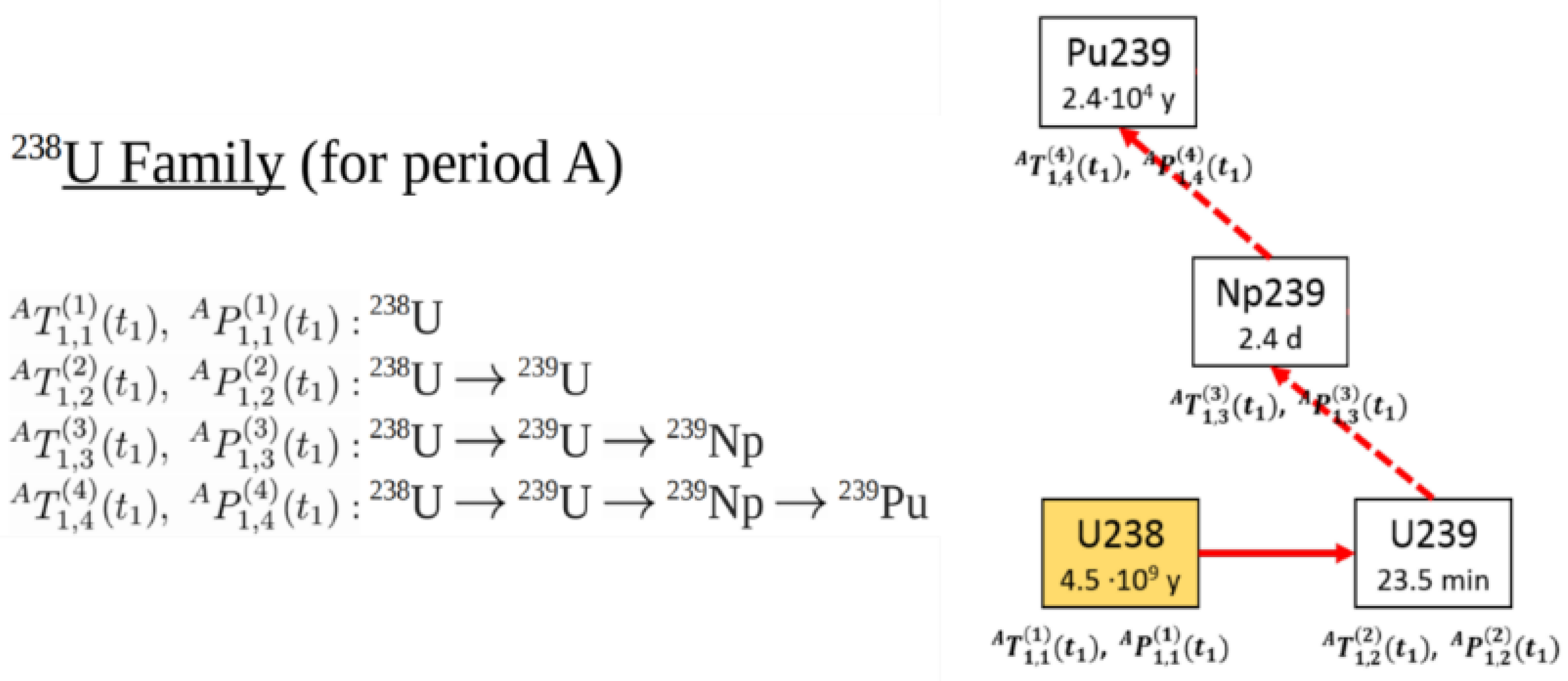
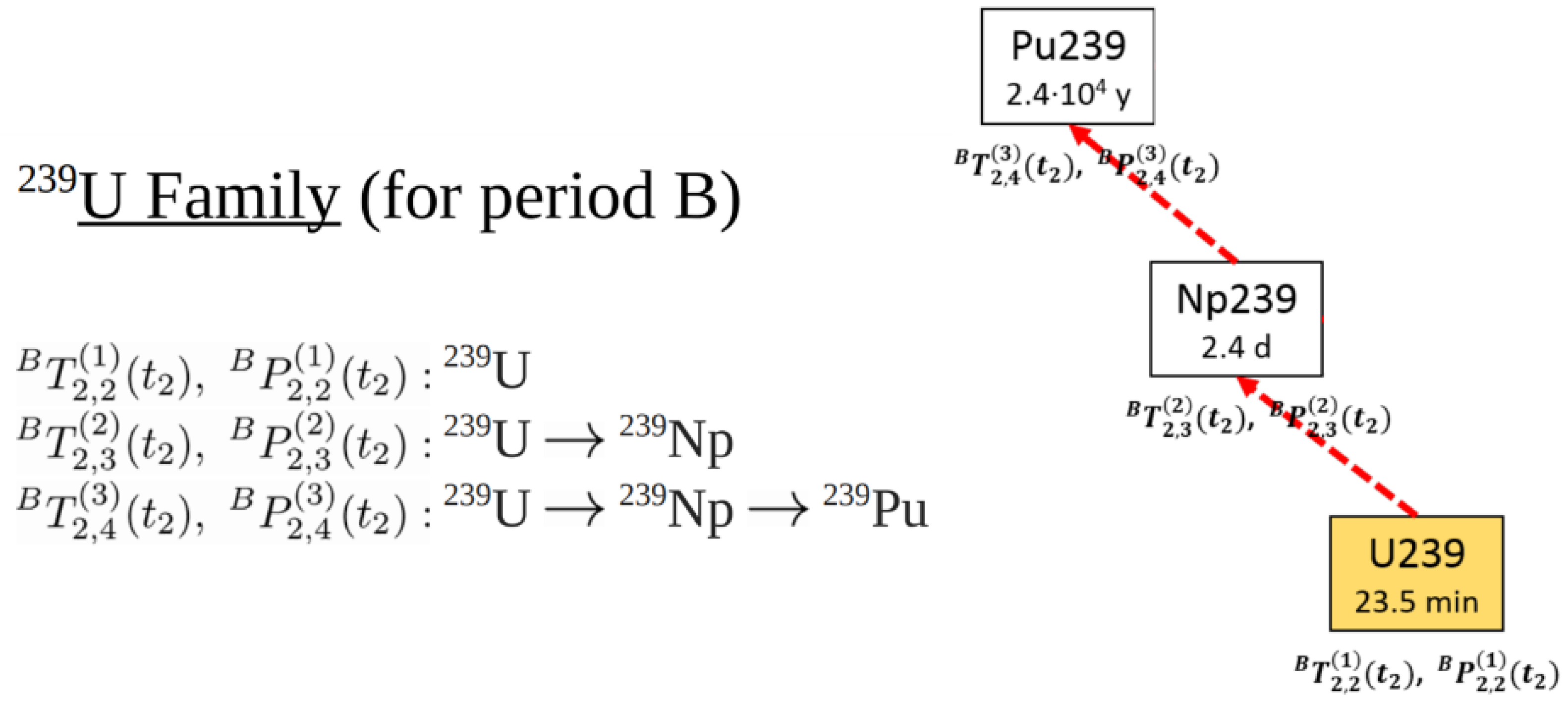
Chain transmutation pattern: 238U (survival)
A: 238UB: 238U T A 1 , 1 ( 1 ) ( t 1 ) · T B 1 , 1 ( 1 ) ( t 2 )
T A , B 1 , 1 ( 1 ) ( t 1 + t 2 ) = T A 1 , 1 ( 1 ) ( t 1 ) · T B 1 , 1 ( 1 ) ( t 2 )
P A , B 1 , 1 ( 1 ) ( t 1 + t 2 ) = P A 1 , 1 ( 1 ) ( t 1 ) + T A 1 , 1 ( 1 ) ( t 1 ) · P B 1 , 1 ( 1 ) ( t 2 )
Chain transmutation pattern: 238U→239U
A: 238U B: 238U→239U T A 1 , 1 ( 1 ) ( t 1 ) · T B 1 , 2 ( 2 ) ( t 2 )
A: 238U→239U B: 239U T A 1 , 2 ( 2 ) ( t 1 ) · T B 2 , 2 ( 1 ) ( t 2 )
T A , B 1 , 2 ( 2 ) ( t 1 + t 2 ) = T A 1 , 1 ( 1 ) ( t 1 ) · T B 1 , 2 ( 2 ) ( t 2 ) + T A 1 , 2 ( 2 ) ( t 1 ) · T B 2 , 2 ( 1 ) ( t 2 )
P A , B 1 , 2 ( 2 ) ( t 1 + t 2 ) = P A 1 , 2 ( 2 ) ( t 1 ) + T A 1 , 1 ( 1 ) ( t 1 ) · P B 1 , 2 ( 2 ) ( t 2 ) + T A 1 , 2 ( 2 ) ( t 1 ) · P B 2 , 2 ( 1 ) ( t 2 )
Chain transmutation pattern: 238U→239U→239Np
A: 238U B: 238U→239U→239Np T A 1 , 1 ( 1 ) ( t 1 ) · T B 1 , 3 ( 3 ) ( t 2 )
A: 238U→239U B: 239U→239Np T A 1 , 2 ( 2 ) ( t 1 ) · T B 2 , 3 ( 2 ) ( t 2 )
A: 238U→239U→239Np B: 239Np T A 1 , 3 ( 3 ) ( t 1 ) · T B 3 , 3 ( 1 ) ( t 2 )
T A , B 1 , 3 ( 3 ) ( t 1 + t 2 ) = T A 1 , 1 ( 1 ) ( t 1 ) · T B 1 , 3 ( 3 ) ( t 2 ) + T A 1 , 2 ( 2 ) ( t 1 ) · T B 2 , 3 ( 2 ) ( t 2 ) + T A 1 , 3 ( 3 ) ( t 1 ) · T B 3 , 3 ( 1 ) ( t 2 )
P A , B 1 , 3 ( 3 ) ( t 1 + t 2 ) = P A 1 , 3 ( 3 ) ( t 1 ) + T A 1 , 1 ( 1 ) ( t 1 ) · P B 1 , 3 ( 3 ) ( t 2 ) + T A 1 , 2 ( 2 ) ( t 1 ) · P B 2 , 3 ( 2 ) ( t 2 ) + T A 1 , 3 ( 3 ) ( t 1 ) · P B 3 , 3 ( 1 ) ( t 2 )
Chain transmutation pattern: 238U→239U→239Np→239Pu
A: 238U B: 238U→239U→239Np→239Pu T A 1 , 1 ( 1 ) ( t 1 ) · T B 1 , 4 ( 4 ) ( t 2 )
A: 238U→239U B: 239U→239Np→239Pu T A 1 , 2 ( 2 ) ( t 1 ) · T B 2 , 4 ( 3 ) ( t 2 )
A: 238U→239U→239Np B: 239Np→239Pu T A 1 , 3 ( 3 ) ( t 1 ) · T B 3 , 4 ( 2 ) ( t 2 )
A: 238U→239U→239Np→239Pu B: 239Pu T A 1 , 4 ( 4 ) ( t 1 ) · T B 4 , 4 ( 1 ) ( t 2 )
T A , B 1 , 4 ( 4 ) ( t 1 + t 2 ) = T A 1 , 1 ( 1 ) ( t 1 ) · T B 1 , 4 ( 4 ) ( t 2 ) + T A 1 , 2 ( 2 ) ( t 1 ) · T B 2 , 4 ( 3 ) ( t 2 ) + T A 1 , 3 ( 3 ) ( t 1 ) · T B 3 , 4 ( 2 ) ( t 2 ) + T A 1 , 4 ( 4 ) ( t 1 ) · T B 4 , 4 ( 1 ) ( t 2 )
P A , B 1 , 4 ( 4 ) ( t 1 + t 2 ) = P A 1 , 4 ( 4 ) ( t 1 ) + T A 1 , 1 ( 1 ) ( t 1 ) · P B 1 , 4 ( 4 ) ( t 2 ) + T A 1 , 2 ( 2 ) ( t 1 ) · P B 2 , 4 ( 3 ) ( t 2 ) + T A 1 , 3 ( 3 ) ( t 1 ) · P B 3 , 4 ( 4 ) ( t 2 ) + T A 1 , 4 ( 4 ) ( t 1 ) · P B 4 , 4 ( 1 ) ( t 2 )
Publisher’s Note: MDPI stays neutral with regard to jurisdictional claims in published maps and institutional affiliations.

