Modeling Cycle-to-Cycle Variations of a Spark-Ignited Gas Engine Using Artificial Flow Fields Generated by a Variational Autoencoder

Abstract

A deeper understanding of the physical nature of cycle-to-cycle variations (CCV) in internal combustion engines (ICE) as well as reliable simulation strategies to predict these CCV are indispensable for the development of modern highly efficient combustion engines. Since the combustion process in ICE strongly depends on the turbulent flow field in the cylinder and, for spark-ignited engines, especially around the spark plug, the prediction of CCV using computational fluid dynamics (CFD) is limited to the modeling of turbulent flows. One possible way to determine CCV is by applying large eddy simulation (LES), whose potential in this field has already been shown despite its drawback of requiring considerable computational time and resources. This paper presents a novel strategy based on unsteady Reynolds-averaged Navier–Stokes (uRANS) CFD in combination with variational autoencoders (VAEs). A VAE is trained with flow field data from presimulated cycles at a specific crank angle. Then, the VAE can be used to generate artificial flow fields that serve to initialize new CFD simulations of the combustion process. With this novel approach, a high number of individual cycles can be simulated in a fraction of the time that LES needs for the same amount of cycles. Since the VAE is trained on data from presimulated cycles, the physical information of the cycles is transferred to the generated artificial cycles.

1. Introduction

Research and development in the field of internal combustion engines (ICE) seems to be outdated given the recent announcements by OEMs that they will stop selling cars with ICE and the EU’s ambitious Green Deal and Fit for 55. Nevertheless, ICE technology is not restricted to passenger cars, and there are many more areas of application including the transportation of goods [1], shipping [2], and energy production in remote areas [3] in which ICE will likely continue to play an important role. Furthermore, e-fuels as well as carbon-free fuels such as ammonia or hydrogen will permit the continued use of ICE applications while keeping greenhouse gas emissions on a level comparable to other energy conversion technologies.

One common focus of current and future engine research is the investigation of cycle-to-cycle variations (CCV). The goal of engine manufacturers is to develop highly efficient, low-emission engines, especially for spark-ignited (SI) engines, and the way to achieve this is by using lean burn combustion concepts or exhaust gas recirculation. These technologies significantly promote combustion instabilities as discussed in the reviews of Young [4], Ozdor et al. [5], and Maurya [6]. To a certain extent, the causes of CCV in SI engines are well known. Ranging from physiochemical (e.g., flow field, turbulence, composition), to operational sources (e.g., load, engine speed) to geometric sources (e.g., compression ratio, spark plug properties) [4,5,6,7,8,9], the variety of influencing factors that promote cyclic fluctuations in ICE indicates great challenges in their prediction to develop efficient control strategies for reducing CCV.

Since CCV corresponds to fluctuations in the engine behavior over a certain number of cycles at constant operating conditions, questions may arise as to how to specify CCV and which engine process property is used for quantification. A common approach is to determine the coefficient of variation (CoV) of directly measured quantities: peak firing pressure, location of peak firing pressure, or derived quantities such as the indicated mean effective pressure (IMEP). Recent approaches focus on the early phase of the combustion process and refer to the CoV calculation on combustion progress variables such as the mass fraction burned point at 2% or 10% (MFB2 or MFB10, respectively). If these conditions are used to quantify CCV with experimental data, the increased impact of measurement errors has to be considered compared to the direct usage of the measured cylinder pressure due to the influence of other quantities on their calculation [10,11,12].

An important tool for investigating the sources of CCV in ICE is simulation via computational fluid dynamics (CFD). Simulation makes it possible to examine in detail the turbulent flow and the combustion process (to a certain extent), which otherwise would be nearly impossible or would require enormous effort to obtain from a real engine. Large eddy simulation (LES) has recently become widespread for investigating CCV in ICE [13] and has also found its way from academic to industrial settings. Since computational power has increased significantly in the last few decades, LES has already found its way into industry and everyday CFD. Since LES uses a filtering approach rather than averaging the governing equations upon which unsteady Reynolds-averaged Navier–Stokes (uRANS) is based, it has its advantages in the calculation of fluctuating phenomena such as CCV. Various studies have been conducted that focus on the CCV sources investigated with LES to obtain a sufficiently high resolution of the turbulent structures in the flow field and analyze the influence on flame kernel development and flame propagation [14,15,16,17,18,19,20,21]. To overcome the issue of the significantly high computational cost of conducting consecutive simulation of engine cycles with LES, novel approaches based on perturbing simulation parameters (e.g., initial conditions) permit the execution of cycle simulations in parallel. Studies that apply perturbations to the turbulence intensity or the flow field [22,23] in the combustion chamber have successfully demonstrated the applicability of this methodology. Although these methods show a significant reduction in the computational time for CCV via LES, the parallel execution of the single-cycle simulations requires enormous computational power and, if commercial software is used, a sufficient number of licenses. Furthermore, perturbing the flow field or the turbulence intensity randomly does not initially imply that these fields are physically meaningful. Nevertheless, due to the small amplitude of the induced perturbations, this issue may be ignored. In addition to the LES method, Scarcelli et al. [24] concluded that uRANS turbulence modeling in combination with sufficient fine mesh resolution can be used of CCV in SI engines since most of the underlying effects for CCV can be captured by this method.

The idea behind the present paper is based on the previously mentioned approach of running multiple cycle simulations in parallel instead of consecutively in order to obtain cyclic fluctuations of an ICE via CFD. The difference and thus the novelty of the proposed method are its application of a variational autoencoder (VAE) to generate flow fields and turbulence intensity rather than randomly perturbing them. Thanks to the work of Kingma and Welling [25], VAE has received significant attention in the data science community. As a part of the deep learning-based generative model family, VAEs have proven that they can be applied to generate new artificial images from a branch of trained images and have also been successfully used for data augmentation and source classification in various scientific fields [26,27]. Similar to a classic autoencoder, VAE consists of an encoder, a decoder, and a latent space. The dimensionality of the initial data fed to the encoder, which is commonly represented by a neural network, is reduced followed by the reverse process in the decoder. Since the structures of the data in the latent space are uninterpretable, the use of a classical autoencoder for data augmentation is not feasible. Here, the difference between an autoencoder and a VAE comes into play. VAEs use regularization to enable a regular latent space which leads to inferences between decoded points in the latent space and points in their vicinity. As a result, artificial data can be generated by sending new data points from the latent space through the encoder. The present approach uses this feature by feeding flow and turbulent kinetic energy ($TKE$) fields of an engine cylinder into a VAE in order to learn flow features and represent the cylinder flow in low-dimensional space. By changing the latent space values in meaningful ranges and propagating the data through the trained decoder, artificial flow and $TKE$ fields are generated, which serve as initial states for turbulent combustion simulation. Thus, multicycle simulations can be performed without the need to run the low-pressure part of the engine cycle, significantly reducing the computational time. Furthermore, the method also enables the simulation of concurrent cycles in parallel, which was previously mentioned as the significant advantage of the perturbation methods.

The method of generating artificial flow fields by VAE to simulate cyclic variations is demonstrated using a large gas engine. The flow and $TKE$ fields are determined by uRANS simulation and extracted at certain timing of the engine cycle [28]. Furthermore, the preprocessing of the data is described so it may be used in the proposed VAE architecture. A particular emphasis is laid on the validation of the VAE to rule out any misinterpretation of the ability of the proposed method to model cyclic variations. The final model result supports the hypothesis that the VAE approach can be used to generate artificial flow and turbulent kinetic energy fields, which serve as the basis for cycle-to-cycle simulations of ICE. Although the present investigations are based on uRANS turbulence modeling, the methodology is also applicable to LES. In addition to the velocity and $TKE$ fields, other values—for example, residual gas distribution or air–fuel ratio—can be used to extend the approach to further factors that influence cyclic variations.

2. Materials and Methods

2.1. Engine Setup

The basis for the present study is a large gas engine platform with a bore and stroke of 135 mm and 175 mm, respectively, and a displacement of roughly 2.4 dm³. The engine is operated with a premixed gas–air mixture at lean conditions. Full load operating conditions at 1500 min⁻¹ are considered in the investigations described below.

2.2. CFD Simulation Setup

The commercial CFD solver CONVERGE, version 3.0, is used for the simulation. The domain is discretized with a cut-cell Cartesian grid with 2 mm cells in the ports and 1 mm cells in the cylinder during gas exchange and combustion. Wall refinement is applied to better capture near wall effects. Adaptive mesh refinement in the cylinder better captures gradients of velocity and temperature. Turbulence is modeled using the k-$\epsilon$ RNG turbulence model. The time step is adaptively changed to achieve a Courant number of 2–4 during gas exchange and compression. During combustion, the time step remains constant at 10⁻⁶ s, and a reduced NUI Galway reaction mechanism for natural gas is used [29].

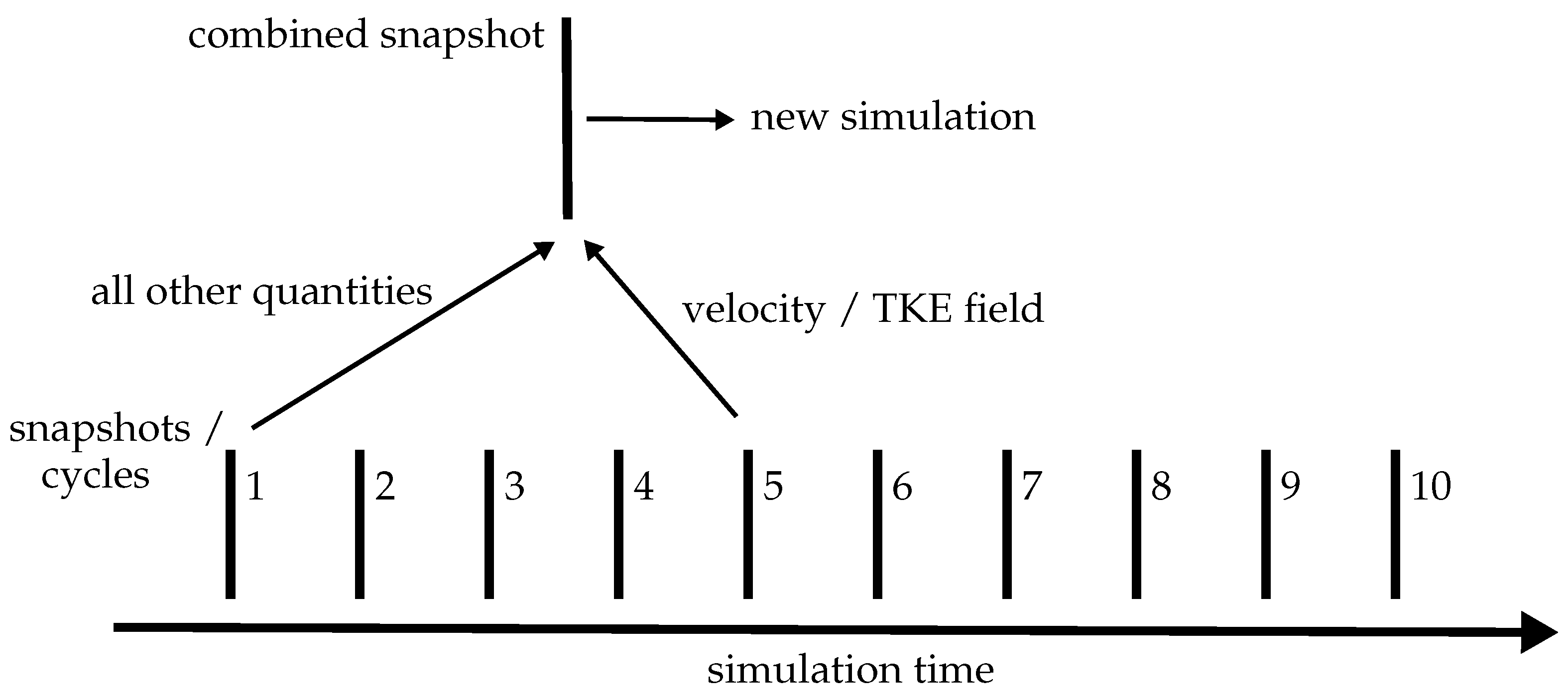
2.3. Multicycle Simulations

To produce the flow fields that act as the source for training the VAE, CFD simulations of eleven consecutive engine cycles are performed using the uRANS method according to approaches from past studies that are found in the literature [24,30,31]. By ignoring the first cycle to avoid initialization effects, ten cycles remain from which the flow field in each coordinate direction as well as the $TKE$ field at 5 CAD before spark timing are used for the VAE training process. Since Gößnitzer and Givler [28] provide a detailed description of the method for how to extract the flow field and recombine the snapshots, only a brief explanation is given at this point. The extraction of the desired fields is restricted to a cylindrical domain in the vicinity of the spark plug so that the data used to train the VAE remain within reasonable limits. Although the flow field in this region usually has a major impact on cyclic variations, the VAE can also be trained by fields from throughout the entire cylinder.

For the VAE to be able to process the data, the number of data points per field has to be constant for all variables and cyclic fields. This is not guaranteed due to the use of AMR. Thus, each velocity and $TKE$ snapshot is mapped on a common grid, yielding a uniform number of values for each field. To ignore the influence of pressure, temperature, and gas composition, the corresponding fields from the first cycle are taken and combined with the snapshot velocity and $TKE$ fields of the other nine cycles. The resulting combined snapshots are rerun, and the simulated cylinder pressure as well as the rate of heat release are used in the evaluation of the proposed approach. Figure 1 visualizes how the evaluation data are generated.

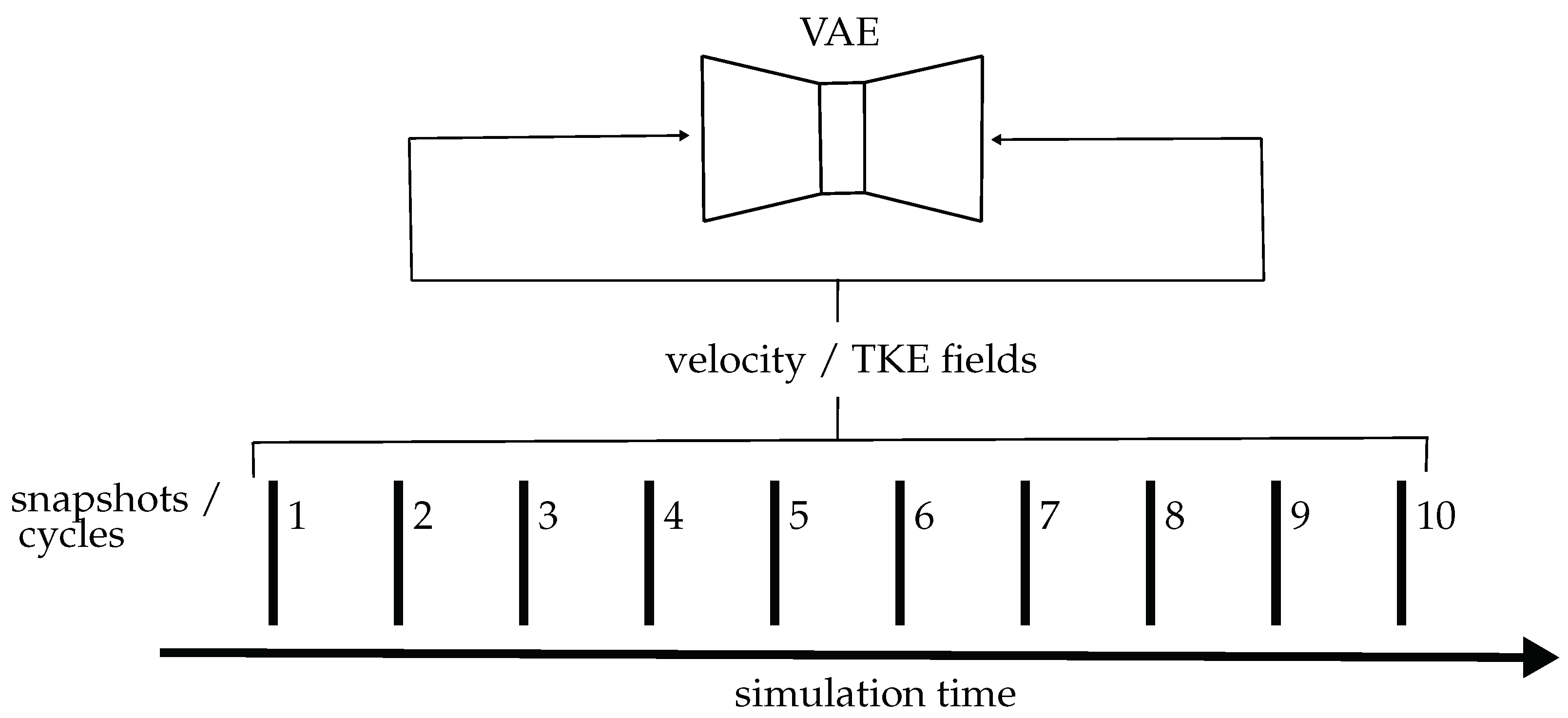
2.4. Variational Autoencoder

A variational autoencoder is a type of deep generative model that has received considerable attention in recent years due to its ability to produce high-quality synthetic data samples for various domains. An autoencoder is typically split into two connected segments, namely the encoder and the decoder. The effective purpose of the encoder is dimensionality reduction of the input data, which creates a downscaled representation in a latent space of a predefined size. Then, the decoder upsamples this compressed representation back to the original input size [32]. The training process is governed by backpropagation of the reconstruction loss, which is calculated as a customizable metric between the original input data and the decoder output, e.g., mean squared error (MSE).

While simpler autoencoder architectures, which take this latent space as unaltered input for the decoder portion of the model, have been used effectively for image denoising [33], anomaly detection [34], dimensionality reduction [35], or feature extraction [36], they lack the capacity to generate synthetic data resembling their inputs. Hence, the concept of VAE introduces an additional concept to the latent space [37]. Instead of directly propagating the low-dimensional representation to the decoder, it is used to define a Gaussian distribution. This is typically done by receiving two outputs per latent space parameter that describe the mean and standard deviations of the distribution. Samples taken from these distributions, i.e., the actual latent space, are then used as inputs for the decoder.

Instead of reducing input dimensionality to distinct vectors for every sample propagated through the encoder, the model learns a distribution for the latent variable, which is parametrized differently for every input image. As an additional boundary condition of the model, the distributions defined via the latent space are constrained to be as close to a standard Gaussian (zero mean and unit variance) as possible. This is implemented via a second term that complements the reconstruction loss for a VAE, the Kullback–Leibler divergence, which results in a regularization of the latent space:

$$Los{s}_{VAE}=Los{s}_{reconstruction}+\beta ·KL\left[\mathcal{N}({\mathit{\mu }}_x,{\mathsf{\Sigma }}_x),\mathcal{N}(\mathbf{0},\mathbf{1})\right]$$

(1)

with ${\mathit{\mu }}_x$ and ${\mathsf{\Sigma }}_x$ representing the encoded mean and covariance matrices, respectively, in a given training example x, and $\beta$ acting as a parameter boosting latent space disentanglement, which is discussed below. This effectively makes it possible to generate new synthetic data resembling the training data by sampling new inputs for the decoder from the distributions defined via the learned examples. Without this form of regularization [37], parameters within the latent space can be encoded too far apart from each other, thereby losing the factor of continuity necessary for generating realistic synthetic data. Hence, there is an elevated risk that conventional autoencoders will generate meaningless data when the decoder inputs are randomly sampled within the unregularized latent space.

The parameter $\beta$ in the equation represents a manually chosen factor for the Kullback–Leibler divergence term. While the parameter was initially introduced as a value greater than 1 to enhance disentanglement of the latent variables, this can negatively influence the model’s reconstruction quality [38]. However, it has been shown that $\beta$ values below 1 can also provide the desired disentanglement with no negative effects on the reconstruction [39]. In conclusion, setting the $\beta$ parameter to 1 will make the model equivalent to a standard VAE.

While VAE architecture (treated in Section 2.4.2) in terms of the width and depth has a considerable impact on various factors including general model performance as well as computational complexity and cost, determination of the latent space size is essential to tuning the efficiency of a model. It has been shown that in the design of autoencoders that exclusively use linear operations, the parameters within the latent space will approximately reflect the modes obtained from principal component analysis (PCA) [40]. Furthermore, PCA is an efficient tool for determining the least amount of information required for maximum explanatory power in work with high-dimensional datasets [41]. For this reason, even though a VAE is generally able to reproduce images more effectively [42], the choice of the number of latent space dimensions in this study was guided by a PCA of each component within the flow field data. The capacity of VAEs to be used as efficient generative models has been previously investigated using similarly complex data [43].

2.4.1. Principal Component Analysis and Latent Space Definition

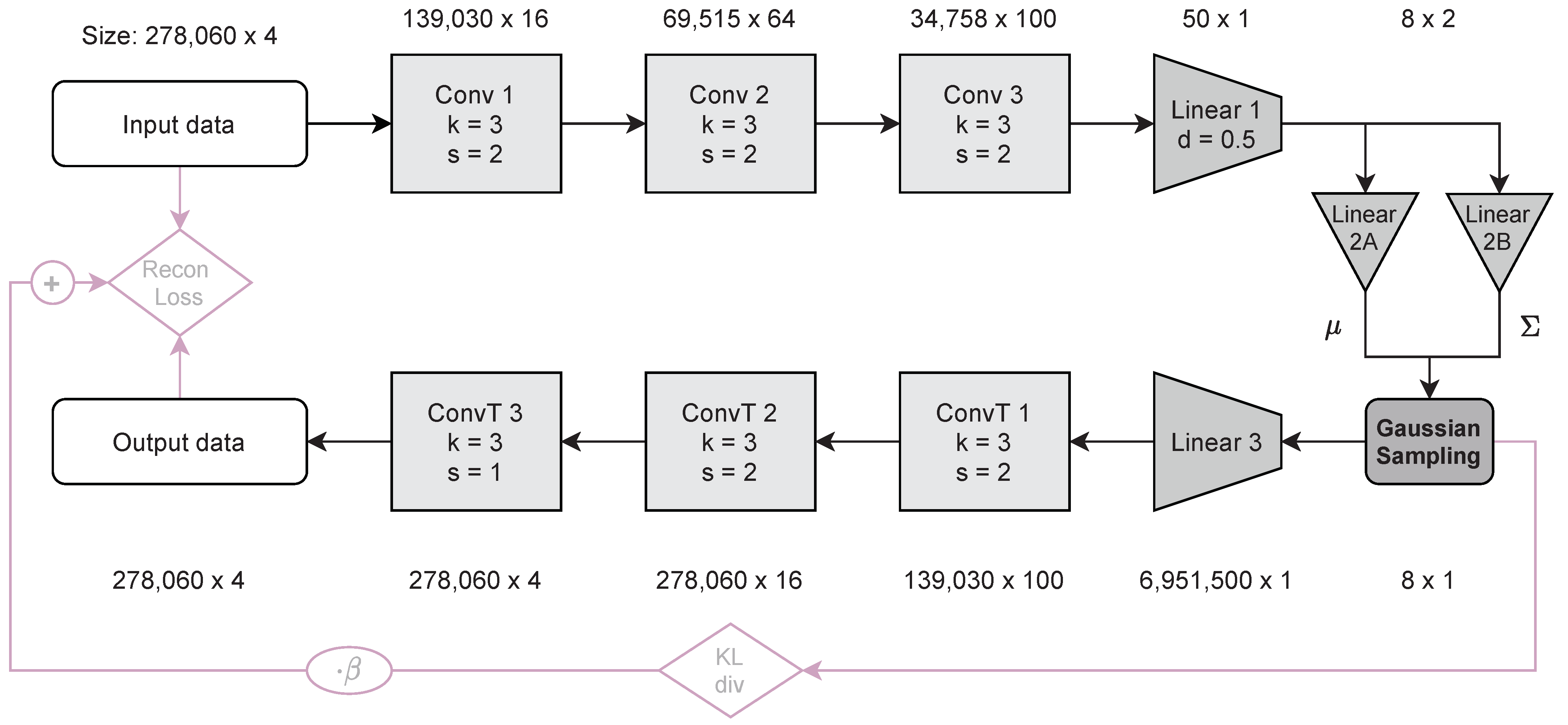
PCA is a widespread method for efficient dimensionality reduction of large datasets under the condition that the statistical information or variability of the initial data is preserved as much as possible. In practice, this is achieved via linear functions of the original data variables, which produce new parameters that maximize variance while being uncorrelated with each other [44]. Hence, the process itself can be described as an eigenvalue problem [45]. These parameters are referred to as principal components (PC).

Due to the underlying composition of the input data in this study, the number of flow fields (10) is much lower than the recorded variables for each recorded quantity (278,060). While this does not interfere with the ability to apply PCA, the number of usable PCs is inherently constrained by the lower of the two values, as it determines the data matrix rank and therefore the number of nonzero eigenvalues. While several specialized forms exist, the PCA in this study was conducted with a singular value decomposition (SVD) of the centered data as described in [46].

The relative explanatory power of each PC is expressed by its explained variance ratio (EVR), which gives the percentage of statistical information it describes. Per definition, this must add up to 1 if the maximum possible number of PCs is computed. To find the minimum amount necessary for a meaningful, lower-dimensional representation of the original data, PCs are first ordered in descending order starting at the highest EVR.

Table 1. Cumulative sum of explained variance ratios, calculated for the specified amount of principal components extracted via distinct PCAs of the original data’s quantities.

# of PCs	u	v	w	$\mathit{TKE}$	Mean
1	0.503	0.350	0.357	0.404	0.404
2	0.689	0.625	0.573	0.568	0.614
3	0.806	0.778	0.702	0.702	0.747
4	0.870	0.851	0.803	0.821	0.836
5	0.918	0.907	0.869	0.889	0.895
6	0.951	0.941	0.920	0.934	0.937
7	0.971	0.969	0.963	0.972	0.969
8	0.987	0.989	0.986	0.987	0.987
9	0.999	0.999	0.999	0.999	0.999
10	1.000	1.000	1.000	1.000	1.000

depicts these EVRs for the specified number of PCs extracted from the flow field data, with each row representing the sum of the respective component EVR and all values before it, i.e., the third row shows the added EVRs of PCs 1, 2, and 3. In this step, the original flow field data were separated into four matrices for each of the columns in the original data with distinct PCAs being conducted for each quantity.

As indicated in the table, the EVR of quantities u and v rises slightly faster as the number of PCs increases than with either w or $TKE$. However, the range of EVRs with seven PCs is already below 1% with a minimum value of 0.963. For the purposes of this study, it was decided that a mean EVR of 0.987 with eight components is sufficient. Accordingly, the dimension of the latent space was also set to eight.

2.4.2. Architecture

Given the high-dimensional nature of the input data with 278,060 variables in each of the four columns for every sample flow field, it was decided to use a convolutional neural network (CNN) architecture for the VAE. CNNs are deep learning models that are made up of multiple convolutional layers, which are followed by at least one linear layer. The former type of layer employs so-called “filters” or “kernels”, which are custom-sized vectors that are trained to extract features from their inputs via eponymous convolution operations. Each layer may consist of any desired number of kernels, each of which generates a distinct output from the same input. Due to this independence, all operations within one convolutional layer can be computed in parallel. Furthermore, the number of trainable parameters is significantly lower than in conventional linear neural network layers. These two aspects provide CNNs with remarkably better computational efficiency while adding the ability to extract multiple features within one single layer, which can also store contextual information within the input. All of these factors contribute to the popularity of CNNs whenever work is done with high-dimensional inputs or data with underlying patterns, for example in image classification [47], sentence modeling [48], or time series anomaly detection [49,50]. Using appropriate parametrization of convolutional layers also allows for efficient dimensionality reduction of input data while simultaneously collecting meaningful features, which is essential for this study.

While the two-dimensional layout of the input data allows the use of 2D kernels as they are employed in image classification, this is not necessary, as the columns are independent from each other. Therefore, the VAE in this study employs 1D kernels with each column representing an individual channel of the input signal. The number of convolutional layers in the encoder was set to three, each of which reduced the input dimension by a factor of two while increasing the amount of kernels per layer before further propagating to two linear layers. This results in a rather high number of trainable parameters, in turn elevating the risk of overfitting, which in generative neural networks describes an instance where the model’s learning process progresses past a tipping point, leading it to specialize on its inputs. Thus, the ability to produce new data becomes increasingly more limited to samples closely resembling the training data. However, since the underlying problem of this study specifically demands for generated data similar to the model inputs, this elevated risk of overfitting is negligible. Following the encoder part of the VAE, the resulting parameters are used to define distributions of the latent space from which the decoder inputs are sampled. The decoder itself essentially represents a mirrored version of the encoder with the exception of only a single linear layer being used before three transposed convolutional layers. Bias terms were used for all linear and convolutional layers within the model. The padding parameter for all convolutional and transposed convolutional layers was set to “same”.

Figure 2 illustrates the VAE architecture.

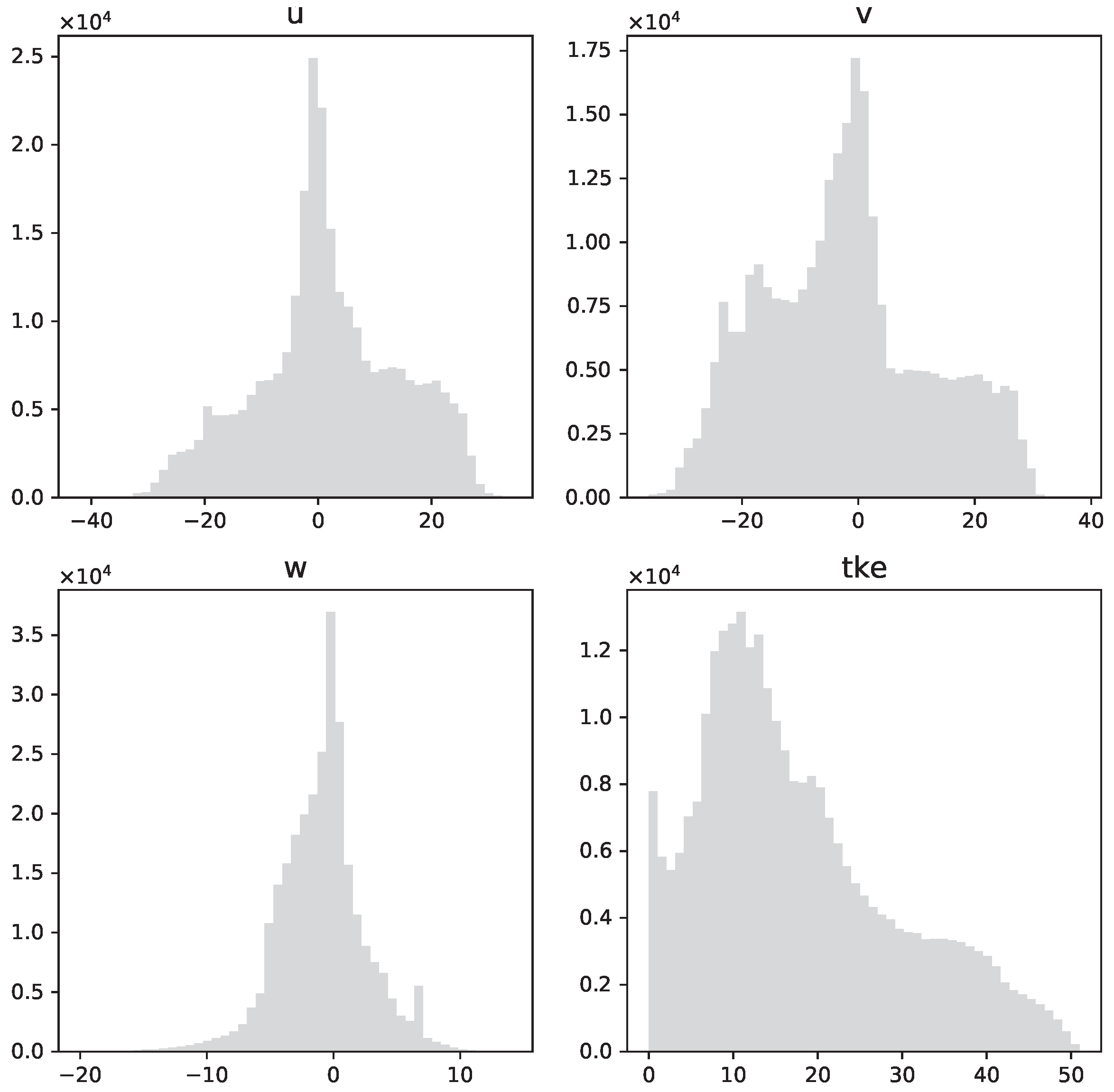
2.4.3. Data Preparation, Hyperparameters, and Training

As with other deep learning methods, the learning efficiency of a VAE is governed by a set of hyperparameters and model buildup decisions, which will be discussed in this section.

To begin with, the input data need to be preprocessed for optimum compatibility with the neural network. Figure 3 illustrates the underlying distribution of each quantity in the input data. As can be observed, u, v, and w are centered around zero, while $TKE$ by definition can only take positive values. To enhance the processability of input values with respect to the reconstruction problem, it was decided to scale all flow fields in a feature range from $-1$ to 1.

In connection with this scaling, the $tanh$ was chosen as the nonlinear activation function for all convolutional and linear layers within the network, since it processes layer outputs in the same range.

The reconstruction loss was implemented as a mean square error (MSE) loss with ADAM—a stochastic gradient descent method—as the learning algorithm, as it has been proven to be efficient with high-dimensional data [51]. After initial tests, the learning rate was set to $0.0001$ with an exponential decay rate of $0.5$ and a batch size of three.

The dropout value for the first linear layer of the encoder was set to $0.5$. As mentioned above, the $\beta$ parameter for latent variable disentanglement was set to $0.2$ in order to preserve a high reconstruction accuracy. The model was trained for 500 epochs to ensure the loss would converge. Figure 4 shows the VAE training process using ten velocity and $TKE$ fields of the multicycle simulations.

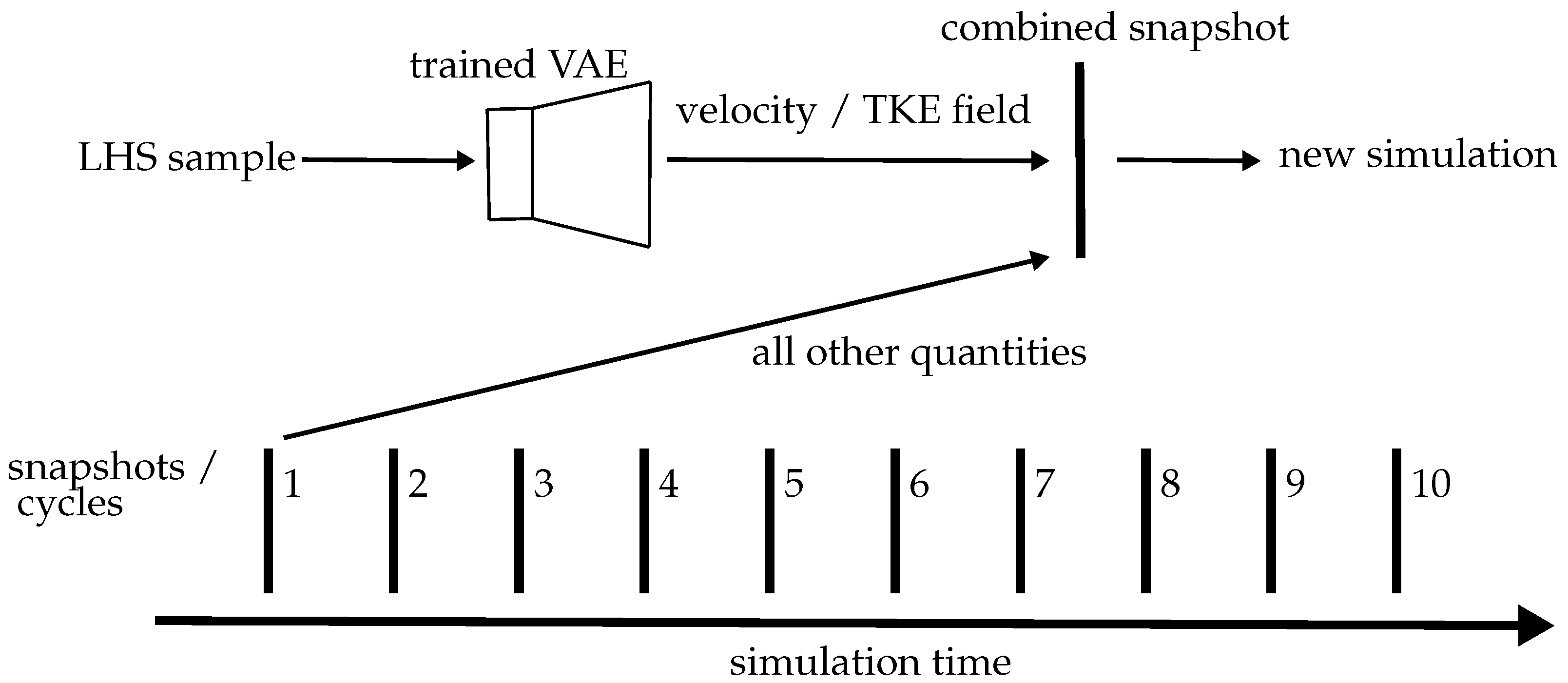
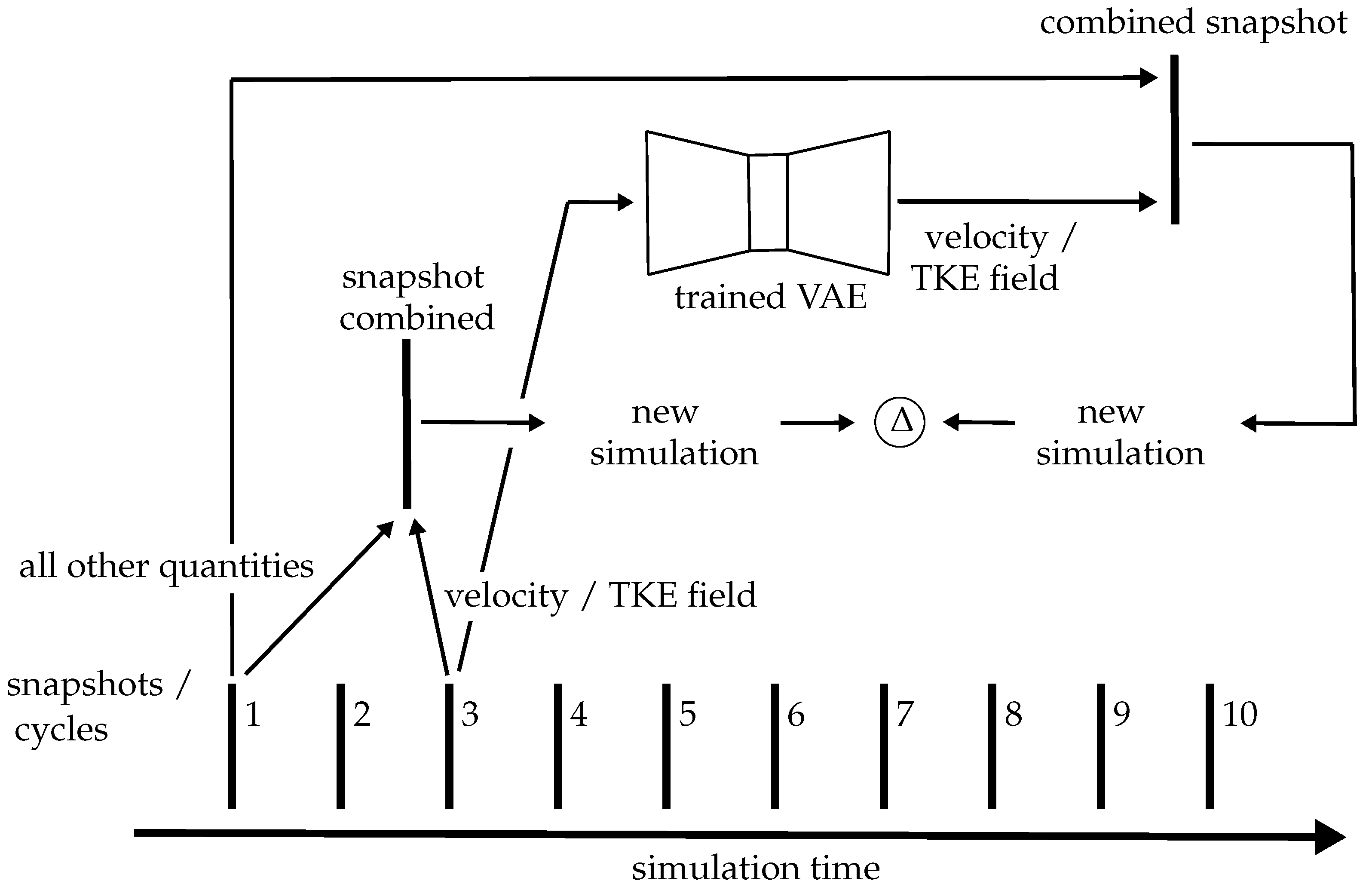
2.5. Artificial Flow Field Generation

After the training process, the VAE can be used to generate new velocity and $TKE$ fields in the considered domain around the spark plug. Only the decoder part of the VAE is required. To create new data in terms of velocity and $TKE$ fields, the encoder requires input values in the dimension of the latent space, which is eight in the present case. The input values are generated with the Latin hypercube sampling (LHS) technique. The VAE training process yields a dimension-reduced transformation of the flow fields in the form of latent space dimension times the number of training flow field values. These values are used to set the boundaries for the LHS process. Therefore, the generated generated artificial fields are forced to lie between the extreme cycles of the training set, and the methodology does not produce physically meaningless cycles. Nevertheless, it is evident that cyclic fluctuations that exceed those in the training set cannot be modeled.

To generate the initial state for the combustion process simulation with the artificial velocity and $TKE$ fields, a methodology similar to the one described earlier for combining snapshots is applied. All quantities of the first cycle are combined with the velocity and $TKE$ field in the cylindrical domain around the spark plug generated by the VAE. Figure 5 illustrates the artificial flow field generation.

3. Results

To maintain confidentiality, the reported data in terms of in-cylinder variables is normalized. The in-cylinder peak pressures are normalized to the minimum and maximum peak pressures. In other words, peak pressures of 100% and 0% correspond to the highest and lowest peak pressure, respectively, and the reported absolute crank angle degrees are normalized with respect to the ignition timing; i.e., all reported absolute crank angle degrees in this paper are relative to the ignition.

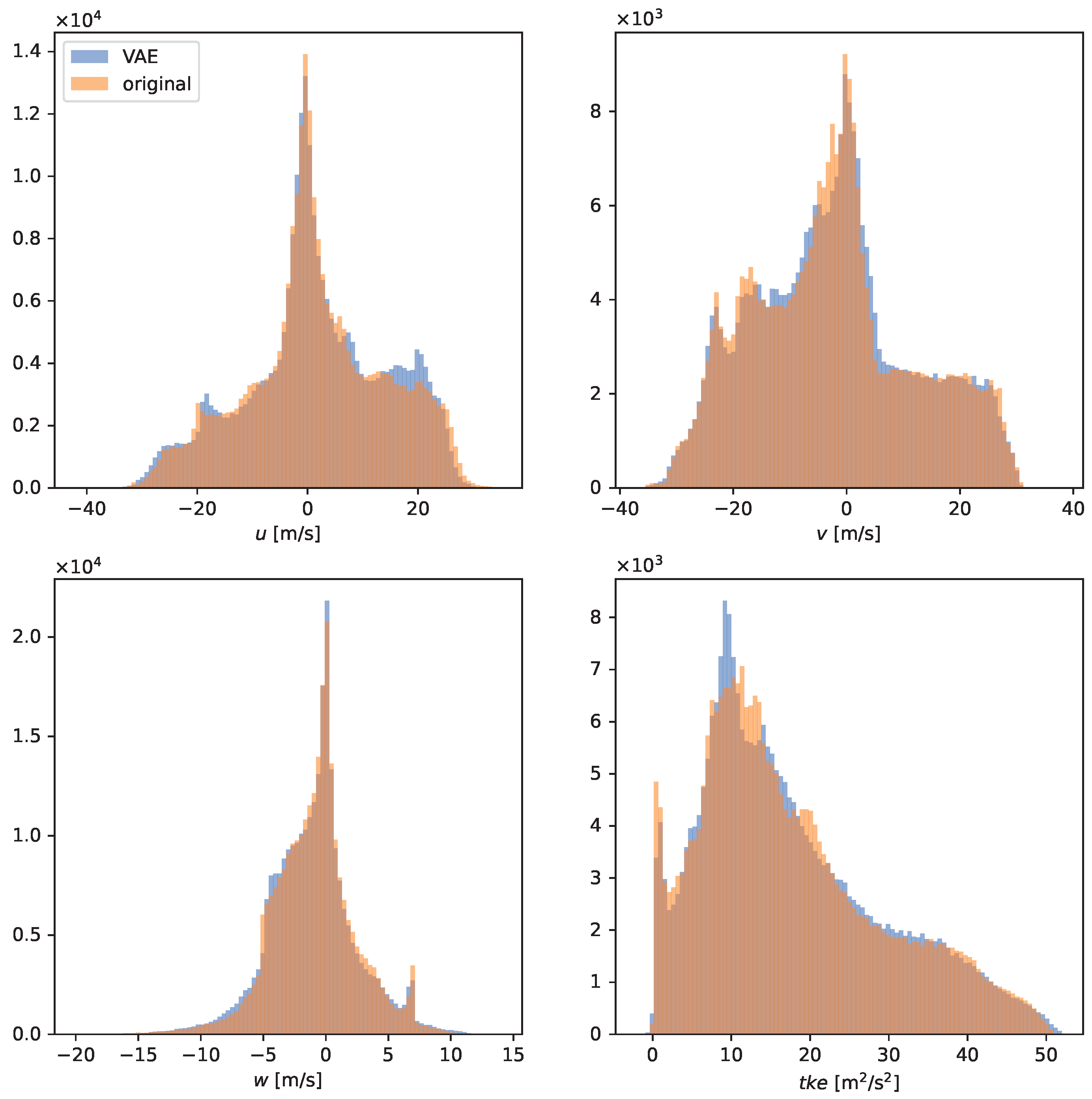
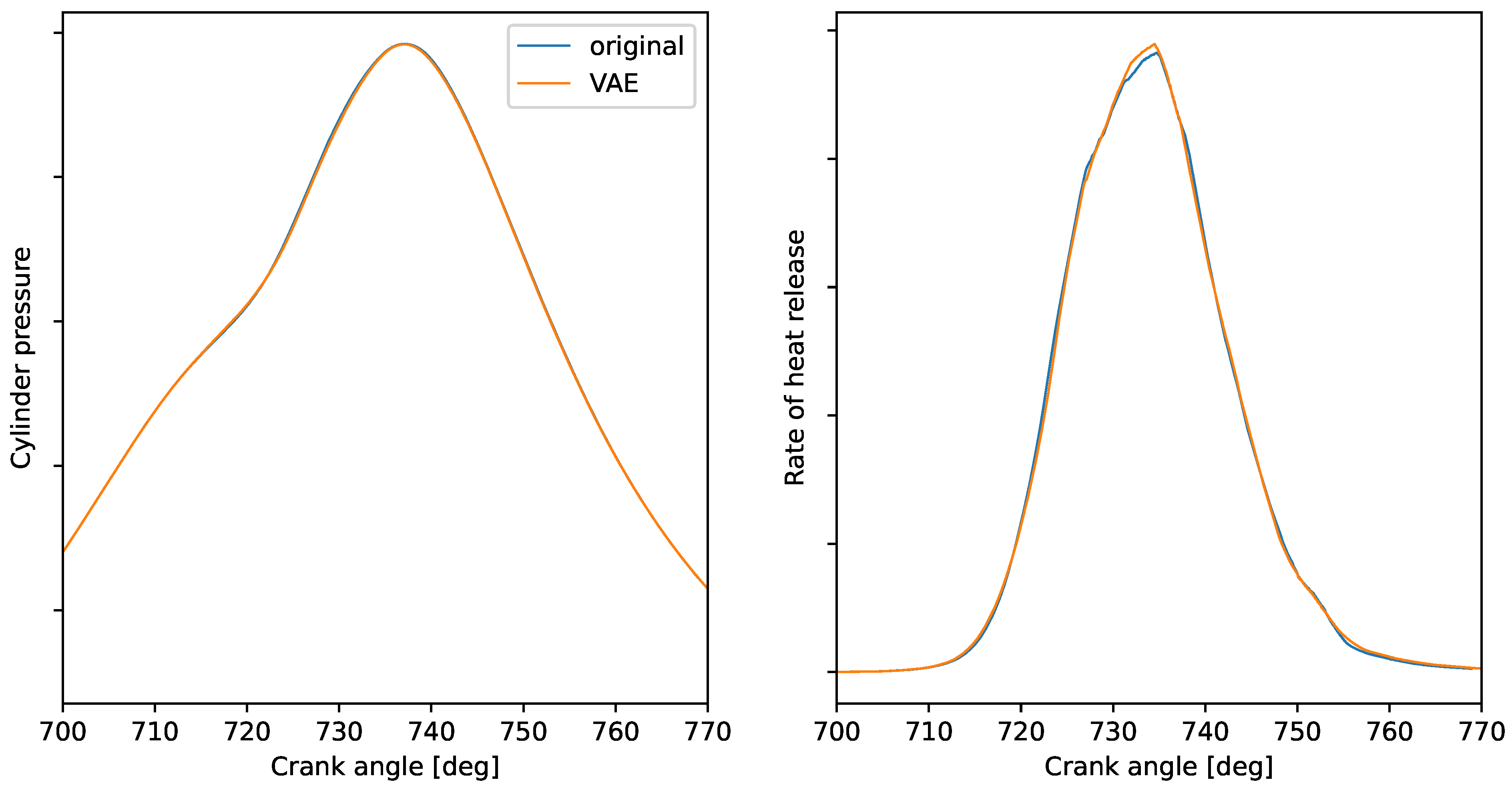
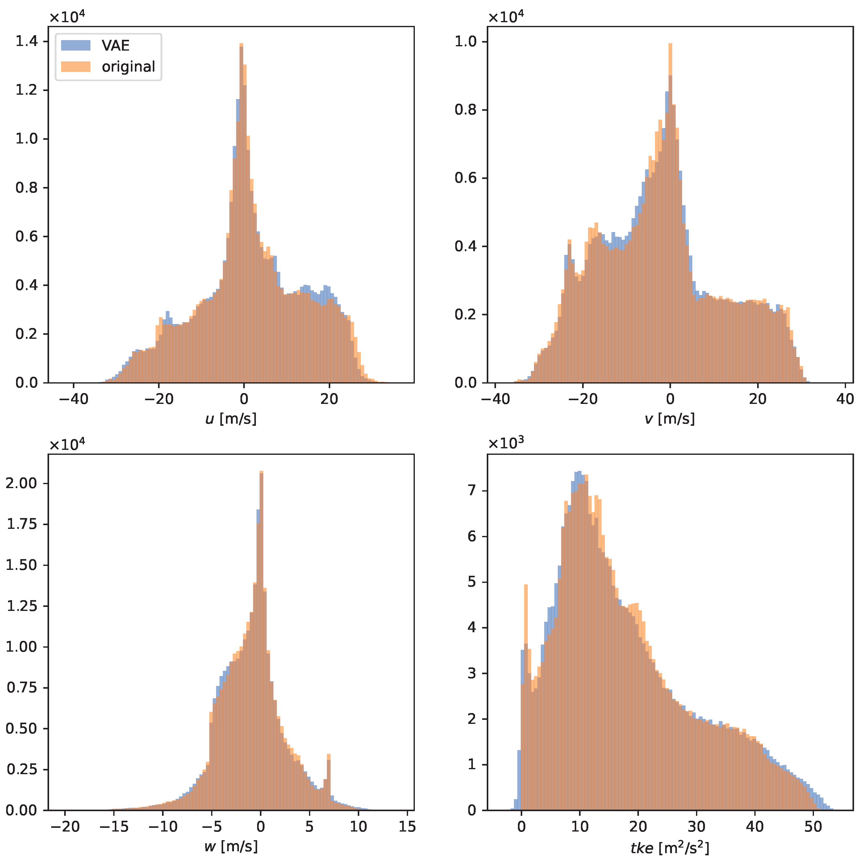
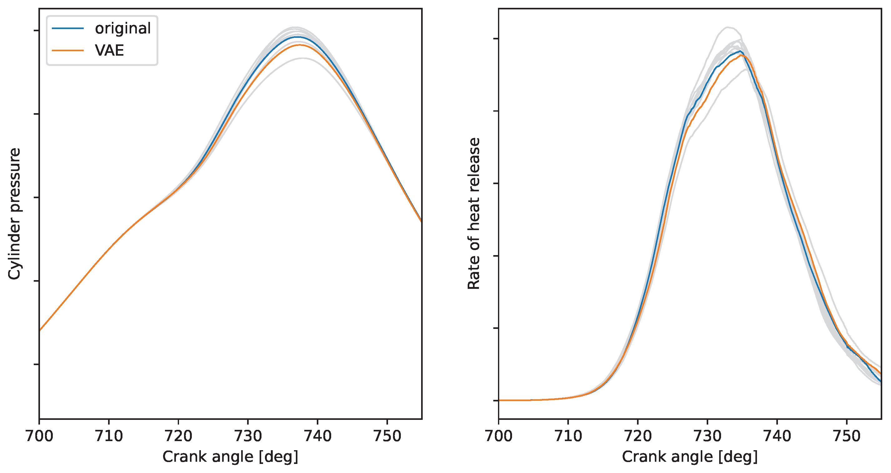
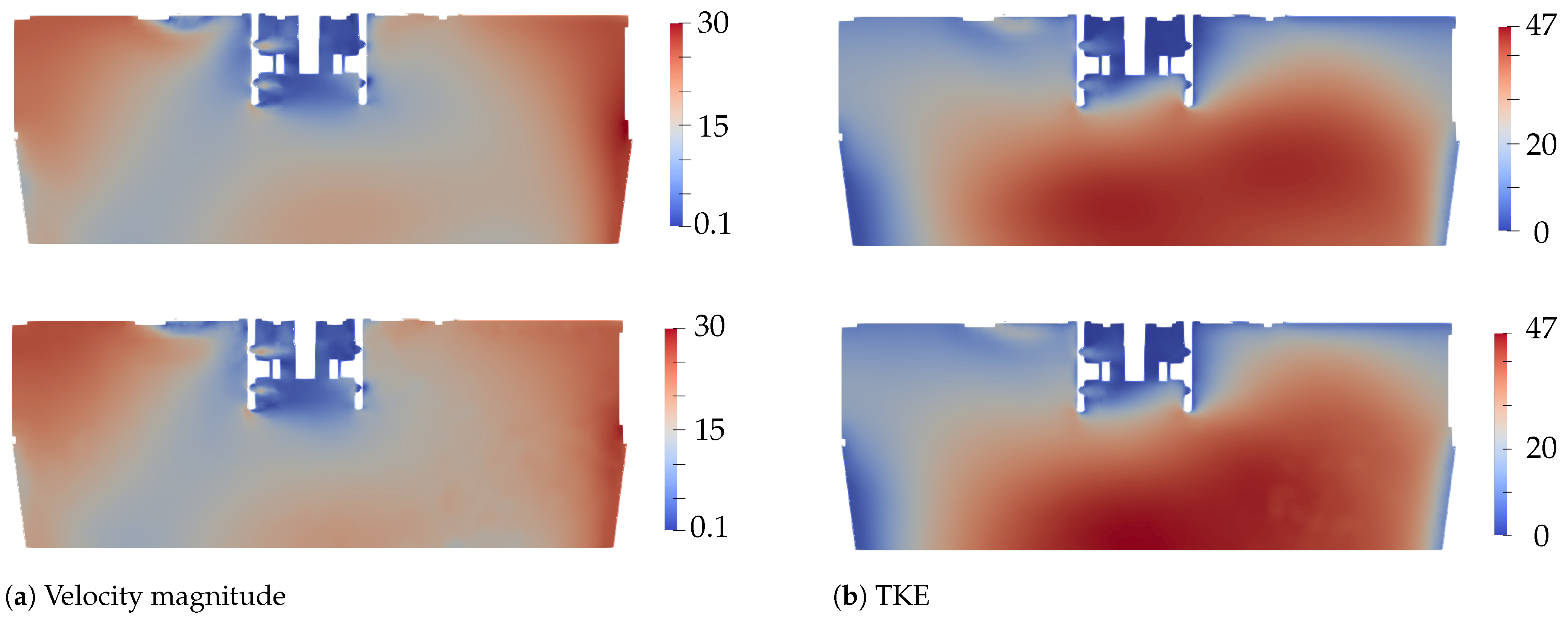
3.1. Model Validation

As described in the methodology section, the present approach is based on combustion process simulation with flow field initial states generated by a VAE. The artificial velocity and $TKE$ fields are produced by LHS values, which are processed by the decoder part of the trained VAE. A validation procedure according to Figure 6 is applied to exclude the possibility of the generation of flow fields that differ from the training set fields from data processing with a poorly trained VAE. Therefore, an arbitrary flow field of the test set is used (cycle 3 in the present case) and processed by the entire VAE, covering the encoder and decoder parts. If the VAE is trained well on the flow fields of the test set, the VAE output corresponds to the given input. In the technique that combines flow fields with quantities of other cycle snapshots described above, the original velocity and $TKE$ fields as well as the VAE output fields are combined with the residual quantities of cycle 1. Finally, both newly generated initial states are used to rerun the ICE combustion process CFD simulation, and the results for cylinder pressure and rate of heat release are compared.

Figure 7 shows the results of the combustion process CFD simulation. As the results indicate, the initial fields reconstructed by the trained VAE yield a congruent in-cylinder pressure trace and an almost congruent rate of heat release. Based on these results, it is concluded that the VAE is trained well on the given flow fields contained in the training dataset.

A further step in the validation process is the investigation of the value distribution of the desired field quantity. Since the information from qualitative analysis of the deviation between the original field and the VAE reconstructed by 3D visualization is only of limited value, an illustration in terms of histograms of the individual field variables is used. As the results in Figure 8 show, the distribution of the original and VAE reconstructed values exhibit very good agreement. The root mean squared error between the original and VAE reconstructed data of the entire variable set is 1.01, which emphasizes the assumption of a well-trained VAE.

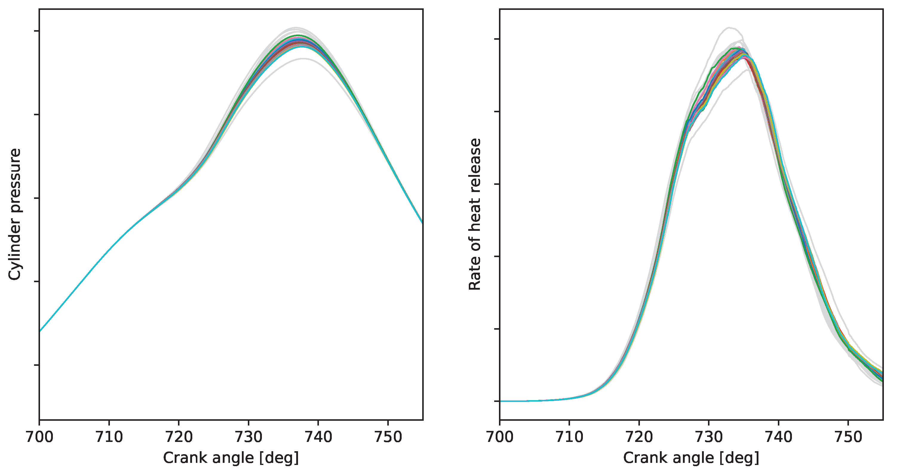
3.2. Artificial Cyclic Variations

The trained VAE is used to generate 20 artificial initial velocity as well as $TKE$ fields with LHS. Through the application of the field combination methodology described above, the artificial fields are combined with the residual quantities of cycle 1 to yield 20 initial states and thus 20 combustion process CFD simulations. To provide detailed insight into the VAE data generation, the following analysis focuses on one specific VAE generated flow field and cycle 3 of the multicycle set used in the validation step. Figure 9 shows the in-cylinder pressure trace and the rate of heat release of the original multicycle set (cycle 3 is highlighted) as well as one artificial cycle based on the VAE generated flow fields. The results indicate the deviation between cycle 3 and the artificial generated cycle, which proves the ability of the VAE to generate velocity and $TKE$ fields that further lead to physically meaningful cycles. A quantitative analysis of the results yields a peak cylinder pressure ($p_{\max }$) of 68.6% for cycle 3 and 42.6% for the artificial cycle while 50% fuel mass fraction burned (MFB_50%) values are 33.5 CAD for cycle 3 and 33.8 CAD for the artificial cycle.

The histogram illustration (Figure 10) is also employed to point out the difference between the velocity and $TKE$ fields of cycle 3 of the original data set and the artificial data generated by the VAE. Although the main characteristic of the distribution was maintained by the VAE, which is required to obtain physically meaningful flow fields, slight differences can be identified. Examples can be seen in the u field at the vicinity of 20 m/s or $TKE$ in the vicinity of 15 m²/s².

In order to prove the physical correctness and the conservation of the flow characteristics of the original data from the VAE, Figure 11 shows the velocity magnitude and $TKE$ in a cut through the middle plane of the considered domain. It can be clearly seen that the flow fields are similar but have slight deviations in some regions. Hence, the VAE is able to generate velocity and $TKE$ fields that are completely new but very similar to the original fields obtained from multicycle CFD simulation.

Figure 12 shows the final results of the multicycle simulations using the original flow field data and the artificial flow field data generated by the VAE. The results indicate that the artificial velocity and $TKE$ fields obtained by the VAE yield meaningful results that fall within the range of the original cycle data used for the VAE training. However, the cyclic variation range of the 20 artificial cycles is not as pronounced as that of the original cycles. The peak pressure $p_{\max }$ ranges from 38.4% to 74.8% and MFB_50% ranges from 33.1 to 34.1 CAD. In terms of CoV, the original data set has a 1.69% peak pressure and 1.29% MFB_50%, and the artificial cycles have 0.65% peak pressure and 0.71% MFB_50%. From the CoV difference between the original and artificial cycles, it can be concluded that the VAE tends to generalize in the training process, and thus, extreme values are less conserved. This observed compression of the VAE’s generative degrees of freedom can be counteracted by measures such as early stopping, amplification of the discussed latent space disentanglement, or dedicated curation of the training data to contain a close to uniform distribution of more and less extreme samples. However, all of these strategies have to be carefully balanced to not interfere with the overall quality of reconstructed flow fields and thus require a large number of experiments. Nevertheless, the results prove the potential of the present approach.

4. Summary and Conclusions

This paper has presented a novel method for generating artificial flow fields that can be used to initialize ICE combustion process CFD simulation. The method uses a VAE to generate flow field data, specifically velocity and $TKE$. To train the VAE, flow fields are extracted from multicycle CFD simulations at a specific crank angle. The data for this study were generated by RANS CFD simulations, but the methodology is also applicable to LES-generated flow field data. To validate the training quality of the VAE on the original velocity and $TKE$ fields, the reconstruction of one of the original cycle flow fields has been investigated and shown to be valid. The trained VAE has been used to generate 20 artificial velocity and $TKE$ fields, which act as initial states for the same number of CFD simulations of the ICE combustion process. Cyclic fluctuations in terms of peak firing pressure and MFB_50% and have been evaluated, which yield 1.69% and 1.29% for the original multicycle data as well as 0.65% and 0.71% for the VAE-based cycles, respectively. These results indicate a trend for the VAE to generalize the training data, yielding the disappearance of extreme values. Further investigations are necessary to overcome this issue and obtain further agreement between the multicycle data used for training and the generated artificially data. However, the comparison between velocity and $TKE$ fields from the original simulation and the VAE-generated flow fields that apply histograms and flow field illustrations show how the VAE maintains the underlying in-cylinder physics. In comparison to state-of-the art methods that generate initial flow fields for multicycle simulation using random perturbation, the proposed method is able to maintain flow field properties to a great extent.

References

1. Smallbone, A.; Jia, B.; Atkins, P.; Roskilly, A.P. The impact of disruptive powertrain technologies on energy consumption and carbon dioxide emissions from heavy-duty vehicles. Energy Convers. Manag. X 2020, 6, 100030. [Google Scholar] [CrossRef]
2. Ni, P.; Wang, X.; Li, H. A review on regulations, current status, effects and reduction strategies of emissions for marine diesel engines. Fuel 2020, 279, 118477. [Google Scholar] [CrossRef]
3. Guelpa, E.; Bischi, A.; Verda, V.; Chertkov, M.; Lund, H. Towards future infrastructures for sustainable multi-energy systems: A review. Energy 2019, 184, 2–21. [Google Scholar] [CrossRef]
4. Young, M.B. Cyclic Dispersion in the Homogeneous-Charge Spark-Ignition Engine-A Literature Survey. SAE Trans. 1981, 49–73. [Google Scholar] [CrossRef]
5. Ozdor, N.; Dulger, M.; Sher, E. Cyclic Variability in Spark Ignition Engines A Literature Survey. SAE Trans. 1994, 103, 1514–1552. [Google Scholar] [CrossRef]
6. Maurya, R.K. Combustion Stability Analysis. In Reciprocating Engine Combustion Diagnostics: In-Cylinder Pressure Measurement and Analysis; Springer: Cham, Switzerland, 2019; pp. 361–459. [Google Scholar] [CrossRef]
7. Matekunas, F.A. Modes and Measures of Cyclic Combustion Variability. SAE Trans. 1983, 1139–1156. [Google Scholar] [CrossRef]
8. El-Adawy, M.; Heikal, M.R.; A. Aziz, A.R.; Adam, I.K.; Ismael, M.A.; Babiker, M.E.; Baharom, M.B.; Firmansyah; Abidin, E.Z.Z. On the Application of Proper Orthogonal Decomposition (POD) for In-Cylinder Flow Analysis. Energies 2018, 11, 2261. [Google Scholar] [CrossRef] [Green Version]
9. Martinez-Boggio, S.; Merola, S.; Teixeira Lacava, P.; Irimescu, A.; Curto-Risso, P. Effect of Fuel and Air Dilution on Syngas Combustion in an Optical SI Engine. Energies 2019, 12, 1566. [Google Scholar] [CrossRef] [Green Version]
10. Johansson, B. Cycle to Cycle Variations in S.I. Engines-The Effects of Fluid Flow and Gas Composition in the Vicinity of the Spark Plug on Early Combustion. SAE Trans. 1986, 2281–2296. [Google Scholar] [CrossRef] [Green Version]
11. Schiffmann, P. Root Causes of Cyclic Variability of Early Flame Kernels in Spark Ignited Engines. Ph.D. Thesis, University of Michigan, Ann Arbor, MI, USA, 2016. [Google Scholar]
12. Schiffmann, P.; Reuss, D.L.; Sick, V. Empirical investigation of spark-ignited flame-initiation cycle-to-cycle variability in a homogeneous charge reciprocating engine. Int. J. Engine Res. 2018, 19, 491–508. [Google Scholar] [CrossRef]
13. Lauer, T.; Frühhaber, J. Towards a Predictive Simulation of Turbulent Combustion?-An Assessment for Large Internal Combustion Engines. Energies 2021, 14, 43. [Google Scholar] [CrossRef]
14. Vermorel, O.; Richard, S.; Colin, O.; Angelberger, C.; Benkenida, A.; Veynante, D. Towards the understanding of cyclic variability in a spark ignited engine using multi-cycle LES. Combust. Flame 2009, 156, 1525–1541. [Google Scholar] [CrossRef]
15. Liu, K.; Haworth, D.C.; Yang, X.; Gopalakrishnan, V. Large-eddy simulation of motored flow in a two-valve piston engine: POD analysis and cycle-to-cycle variations. Flow Turbul. Combust. 2013, 91, 373–403. [Google Scholar] [CrossRef]
16. Fontanesi, S.; d’Adamo, A.; Rutland, C. Large-Eddy simulation analysis of spark configuration effect on cycle-to-cycle variability of combustion and knock. Int. J. Engine Res. 2015, 16, 403–418. [Google Scholar] [CrossRef] [Green Version]
17. Richard, S.; Dulbecco, A.; Angelberger, C.; Truffin, K. Invited Review: Development of a one-dimensional computational fluid dynamics modeling approach to predict cycle-to-cycle variability in spark-ignition engines based on physical understanding acquired from large-eddy simulation. Int. J. Engine Res. 2015, 16, 379–402. [Google Scholar] [CrossRef]
18. He, C.; Kuenne, G.; Yildar, E.; van Oijen, J.; di Mare, F.; Sadiki, A.; Ding, C.P.; Baum, E.; Peterson, B.; Böhm, B.; et al. Evaluation of the flame propagation within an SI engine using flame imaging and LES. Combust. Theory Model. 2017, 21, 1080–1113. [Google Scholar] [CrossRef] [Green Version]
19. Zhao, L.; Moiz, A.A.; Som, S.; Fogla, N.; Bybee, M.; Wahiduzzaman, S.; Mirzaeian, M.; Millo, F.; Kodavasal, J. Examining the role of flame topologies and in-cylinder flow fields on cyclic variability in spark-ignited engines using large-eddy simulation. Int. J. Engine Res. 2018, 19, 886–904. [Google Scholar] [CrossRef]
20. Ameen, M.M.; Mirzaeian, M.; Millo, F.; Som, S. Numerical Prediction of Cyclic Variability in a Spark Ignition Engine Using a Parallel Large Eddy Simulation Approach. J. Energy Resour. Technol. 2018, 140, 052203. [Google Scholar] [CrossRef] [Green Version]
21. Netzer, C.; Pasternak, M.; Seidel, L.; Ravet, F.; Mauss, F. Computationally efficient prediction of cycle-to-cycle variations in spark-ignition engines. Int. J. Engine Res. 2020, 21, 649–663. [Google Scholar] [CrossRef]
22. Ameen, M.M.; Yang, X.; Kuo, T.W.; Som, S. Parallel methodology to capture cyclic variability in motored engines. Int. J. Engine Res. 2017, 18, 366–377. [Google Scholar] [CrossRef]
23. Accelerating Computational Fluid Dynamics Simulations of Engine Knock Using a Concurrent Cycles Approach, Vol. ASME 2020 Internal Combustion Engine Division Fall Technical Conference, Internal Combustion Engine Division Fall Technical Conference, 2020, V001T06A002. Available online: http://xxx.lanl.gov/abs/https://asmedigitalcollection.asme.org/ICEF/proceedings-pdf/ICEF2020/84034/V001T06A002/6603631/v001t06a002-icef2020-2916.pdf (accessed on 26 January 2022).
24. Scarcelli, R.; Richards, K.; Pomraning, E.; Senecal, P.K.; Wallner, T.; Sevik, J. Cycle-to-Cycle Variations in Multi-Cycle Engine RANS Simulations. In Proceedings of the SAE 2016 World Congress and Exhibition, Detroit, MI, USA, 12–14 April 2016. [Google Scholar] [CrossRef]
25. Kingma, D.; Welling, M. Auto-Encoding Variational Bayes. In Proceedings of the International Conference on Learning Representations, Banff, AB, Canada, 14–16 April 2014. [Google Scholar]
26. Zemouri, R.; Lévesque, M.; Amyot, N.; Hudon, C.; Kokoko, O.; Tahan, S.A. Deep Convolutional Variational Autoencoder as a 2D-Visualization Tool for Partial Discharge Source Classification in Hydrogenerators. IEEE Access 2020, 8, 5438–5454. [Google Scholar] [CrossRef]
27. Kopf, A.; Claassen, M. Latent representation learning in biology and translational medicine. Patterns 2021, 2, 100198. [Google Scholar] [CrossRef]
28. Gößnitzer, C.; Givler, S. A New Method to Determine the Impact of Individual Field Quantities on Cycle-to-Cycle Variations in a Spark-Ignited Gas Engine. Energies 2021, 14, 4136. [Google Scholar] [CrossRef]
29. Bourque, G.; Healy, D.; Curran, H.; Zinner, C.; Kalitan, D.; de Vries, J.; Aul, C.; Petersen, E. Ignition and Flame Speed Kinetics of Two Natural Gas Blends with High Levels of Heavier Hydrocarbons. J. Eng. Gas Turbines Power 2009, 132, 021504. [Google Scholar] [CrossRef]
30. Kosmadakis, G.; Rakopoulos, D.; Arroyo, J.; Moreno, F.; Muñoz, M.; Rakopoulos, C. CFD-based method with an improved ignition model for estimating cyclic variability in a spark-ignition engine fueled with methane. Energy Convers. Manag. 2018, 174, 769–778. [Google Scholar] [CrossRef]
31. Kosmadakis, G.M.; Rakopoulos, C.D. A Fast CFD-Based Methodology for Determining the Cyclic Variability and Its Effects on Performance and Emissions of Spark-Ignition Engines. Energies 2019, 12, 4131. [Google Scholar] [CrossRef] [Green Version]
32. Kramer, M.A. Nonlinear principal component analysis using autoassociative neural networks. AIChE J. 1991, 37, 233–243. [Google Scholar] [CrossRef]
33. Gondara, L. Medical image denoising using convolutional denoising autoencoders. In Proceedings of the 2016 IEEE 16th international conference on data mining workshops (ICDMW), Barcelona, Spain, 12–15 December 2016; pp. 241–246. [Google Scholar]
34. Zhou, C.; Paffenroth, R.C. Anomaly detection with robust deep autoencoders. In Proceedings of the 23rd ACM SIGKDD International Conference on Knowledge Discovery and Data Mining, Halifax, NS, Canada, 13–17 August 2017; pp. 665–674. [Google Scholar]
35. Wang, Y.; Yao, H.; Zhao, S. Auto-encoder based dimensionality reduction. Neurocomputing 2016, 184, 232–242. [Google Scholar] [CrossRef]
36. Xing, C.; Ma, L.; Yang, X. Stacked denoise autoencoder based feature extraction and classification for hyperspectral images. J. Sens. 2016, 2016, 3632943. [Google Scholar] [CrossRef] [Green Version]
37. Kingma, D.P.; Welling, M. An introduction to variational autoencoders. arXiv 2019, arXiv:1906.02691. [Google Scholar]
38. Burgess, C.P.; Higgins, I.; Pal, A.; Matthey, L.; Watters, N.; Desjardins, G.; Lerchner, A. Understanding disentangling in beta-VAE. arXiv 2018, arXiv:1804.03599. [Google Scholar]
39. Shao, H.; Lin, H.; Yang, Q.; Yao, S.; Zhao, H.; Abdelzaher, T. DynamicVAE: Decoupling Reconstruction Error and Disentangled Representation Learning. arXiv 2020, arXiv:2009.06795. [Google Scholar]
40. Oja, E. Simplified neuron model as a principal component analyzer. J. Math. Biol. 1982, 15, 267–273. [Google Scholar] [CrossRef]
41. Vajapeyam, S. Understanding Shannon’s Entropy metric for Information. arXiv 2014, arXiv:1405.2061. [Google Scholar]
42. Du, T.Y. Dimensionality reduction techniques for visualizing morphometric data: Comparing principal component analysis to nonlinear methods. Evol. Biol. 2019, 46, 106–121. [Google Scholar] [CrossRef]
43. Wang, J.; He, C.; Li, R.; Chen, H.; Zhai, C.; Zhang, M. Flow field prediction of supercritical airfoils via variational autoencoder based deep learning framework. Phys. Fluids 2021, 33, 086108. [Google Scholar] [CrossRef]
44. Jolliffe, I.T.; Cadima, J. Principal component analysis: A review and recent developments. Philos. Trans. R. Soc. Math. Phys. Eng. Sci. 2016, 374, 20150202. [Google Scholar] [CrossRef]
45. Hotelling, H. Analysis of a complex of statistical variables into principal components. J. Educ. Psychol. 1933, 24, 417. [Google Scholar] [CrossRef]
46. Tipping, M.E.; Bishop, C.M. Probabilistic principal component analysis. J. R. Stat. Soc. Ser. B 1999, 61, 611–622. [Google Scholar] [CrossRef]
47. Krizhevsky, A.; Sutskever, I.; Hinton, G.E. Imagenet classification with deep convolutional neural networks. Adv. Neural Inf. Process. Syst. 2012, 25, 1097–1105. [Google Scholar] [CrossRef]
48. Kalchbrenner, N.; Grefenstette, E.; Blunsom, P. A convolutional neural network for modelling sentences. arXiv 2014, arXiv:1404.2188. [Google Scholar]
49. Kefalas, A.; Ofner, A.B.; Pirker, G.; Posch, S.; Geiger, B.C.; Wimmer, A. Detection of knocking combustion using the continuous wavelet transformation and a convolutional neural network. Energies 2021, 14, 439. [Google Scholar] [CrossRef]
50. Ofner, A.B.; Kefalas, A.; Posch, S.; Geiger, B.C. Knock Detection in Combustion Engine Time Series Using a Theory-Guided 1D Convolutional Neural Network Approach. IEEE/ASME Trans. Mechatron. 2022; in press. [Google Scholar] [CrossRef]
51. Kingma, D.P.; Ba, J. Adam: A method for stochastic optimization. arXiv 2014, arXiv:1412.6980. [Google Scholar]
Figure 1. Generation of the evaluation data. Here, the velocity and T K E field is extracted from the fifth cycle and combined with all other quantities of the first cycle. Then, the simulation starts at the time that the fifth snapshot was taken.
Energies 15 02325 g001
Figure 2. VAE architecture. The format given for the data dimensions is N × C with N representing the number of variables and C representing the number of channels. k is the kernel size of the filters in the corresponding layer and s is the stride parameter, which defines the step size of the convolution operations within the respective layer.
Energies 15 02325 g002
Figure 3. Distribution of variables in each input data column.
Energies 15 02325 g003
Figure 4. Training of the VAE with velocity and T K E fields in the specified domain of the ten cycles of the multicycle simulation.
Energies 15 02325 g004
Figure 5. Generation of artificial velocity and T K E field using the trained VAE. The corresponding initial field is created by the new fields and the residual fields of cycle one.
Energies 15 02325 g005
Figure 6. Procedure to validate the ability of the VAE to generate meaningful artificial velocity and T K E fields.
Energies 15 02325 g006
Figure 7. In-cylinder combustion process results started with the original and the VAE reconstructed velocity and T K E fields.
Energies 15 02325 g007
Figure 8. Histogram of the velocity components u , v , w , and T K E of the original and VAE reconstructed fields.
Energies 15 02325 g008
Figure 9. In-cylinder combustion process results of the common multicycle simulations and one artificial generated initialization set.
Energies 15 02325 g009
Figure 10. Histogram of the velocity components u , v , w , and T K E of cycle 3 from the original multicycle dataset and the VAE generated fields.
Energies 15 02325 g010
Figure 11. Velocity magnitude and T K E in a cut plane through the spark plug from the original multicycle dataset and the VAE generated fields.
Energies 15 02325 g011
Figure 12. In-cylinder combustion process results of the common multicycle simulation and 20 artificially generated initialization sets.
Energies 15 02325 g012