Abstract
Proton Exchange Membrane Fuel Cells (PEMFCs) are clean energy conversion devices that are widely used in various energy applications. In most applications, the main challenge is accurately estimating the state of health (SoH) of the PEMFCs during dynamic operating conditions. Moreover, their behavior is affected by numerous physical phenomena such as heat and membrane flooding. This paper proposes the design of an observer to estimate the PEMFC parameters. A state-space model is first built from 2D physical equations solved by a finite difference in a discretized space domain. The discretized dynamic model is then used to design an observer based on the continuous-discrete extended Kalman filter. The observer has been validated experimentally and is used to estimate the parameters of a PEMFC under dynamic operating conditions. For several load variations, the results obtained using the proposed observer accurately characterize the dynamic responses of PEMFC in real-time.
1. Introduction
1.1. Background
The need for clean energy production across a number of application sectors is expected to increase significantly in the years to come. Fuel cells (FCs) offer a promising alternative clean-energy conversion technology and are widely used in multiple sectors such as transportation and microgrid systems. More particularly, FCs are also associated with optimizing renewable energy storage. Critically, FCs perform best when supplied with pure hydrogen, which results in zero carbon dioxide emissions [1,2]. However, pure hydrogen production, storage, and distribution represent major obstacles to commercializing fuel cell technology [3,4,5]. Another important challenge associated with FC systems is accurately estimating both their dynamic response in real-time and their state of health (SoH). This paper aims to build an observer to reliably predict these performance indicators.
Based on the kind of electrolytes they employ, there are five types of fuel cells [6]: Proton Exchange Membrane Fuel Cells (PEMFCs), Phosphoric Acid Fuel Cells (PAFCs), Alkaline Fuel Cells (AFCs), Molten Carbonate Fuel Cell (MCFCs), and Solid Oxide Fuel Cells (SOFCs). The PAFC, MCFC, and SOFC operate at high temperatures (220 °C, 650 °C, and up to 1000 °C, respectively), whereas the AFC operating temperature may vary from 50 to 200 °C, offering higher performance than the PEMFC. However, in the case of AFC, the hydrogen and oxygen must be pure for optimal performance [7]. Among the various types of fuel cells, Proton Exchange Membrane Fuel Cells (PEMFCs) offer considerable advantages due to their low operating temperature (generally under 100 °C), high power density, quick start-up capability, and long lifetime [8,9]. This overview of the different types of FC demonstrates the key parameters to consider when evaluating overall performance, notably operating temperature and fuel purity. This work focuses exclusively on PEMFCs.
Building an observer for PEMFCs requires understanding the different physical phenomena within this type of FC, such as voltage losses and voltage/current undershoot. Voltage drop in PEMFCs is caused by activation, mass transport, and ohmic losses, which can be characterized by the Tafel slope, mass transport, and ohmic resistances. These three parameters can be estimated experimentally using two dynamic tests: current steps and current sweeps [10]. The PEMFC voltage undershoot phenomenon happens when the current transiently increases to the next step value. This voltage overshoot/undershoot is mainly affected by certain operating conditions such as diverging water saturation levels appearing particularly after prolonged FC operation. The current does not show undershoot due to the effect of double-layer charge [11,12].
1.2. Literature Review
The main challenge when considering the observer design is the complexity of modeling PEMFC systems given that they are non-linear and multi-variable [13,14], and the fact that several phenomena such as heat and membrane flooding can impact PEMFC performance [15]. Numerous models have been presented in the literature, however, these models are either based on the steady-state representation of FCs or are limited to account for specific dynamic behaviors [16,17,18]. These models are either based on sophisticated mathematical equations [19] or data collected from real-life PEMFC [12]. The authors in [12] developed a semi-empirical, two-dimensional, and non-isothermal dynamic model to simulate the transient response in the step changes of the cell potential. The data used to build the model in [12] was collected from performing a specific number of tests.
Diagnosis methods have been also widely used to monitor the degradations of the fuel cell performance [20,21]. Electrochemical impedance spectroscopy (EIS) was used in [22,23] to identify the Warburg impedance and the constant phase element (CPE), which help to observe the hydration of the electrode-membrane state assembly and SoH. However, EIS is not a very convenient solution for onboard integration because the measurement time is long and the EIS device is expensive. Other papers offered advanced diagnostic techniques, such as particle filter-based prognostics [24,25], but these techniques are based on complicated calculation algorithms which limit their application for real-time estimation of PEMFC parameters. Other observers proposed in [26,27] are based on the measurements of non-electrical quantities such as pressure or oxygen concentration. Spatial discretization was applied on the 2D or 3D models of FCs to solve the models using these measurements.
1.3. Study Aim
Developing a PEMFC observer which is implementable in real-time is extremely important in industrial applications. The model on which this observer is based must take into account the most important phenomena and parameters affecting the FC behavior, such as the double-layer and voltage potentials (concentration, activation, and ohmic polarization). In this paper, a simplified 2D physical model that describes these phenomena with physical equations is derived from the first and second Fick’s law and Tafel’s law. To solve these equations, a spatial discretization method is suggested. The space-discretized dynamic model for gas channels, the Gas Diffusion Layer (GDL), and Catalyst Layer (CL) is then obtained. After that, an observer based on the continuous-discrete extended Kalman filter (EKF) is built using the obtained discretized dynamic model. This observer is based on measuring electrical quantities of voltage and current.
Based on the presented literature review, the observer developed in this paper offers certain advantages over previously proposed observers in that it only uses current and voltage measurements, it does not require complicated measurements, it is able to estimate the dynamic response of the PEMFCs, and it can be implemented in real-time.
1.4. Nomenclature and Constants
All the cell geometry parameters and variables are described in Table 1.

Table 1.
Parameters and variables of PEMFC.
2. Physical Two-Dimensional Model
2.1. Geometry and Assumptions
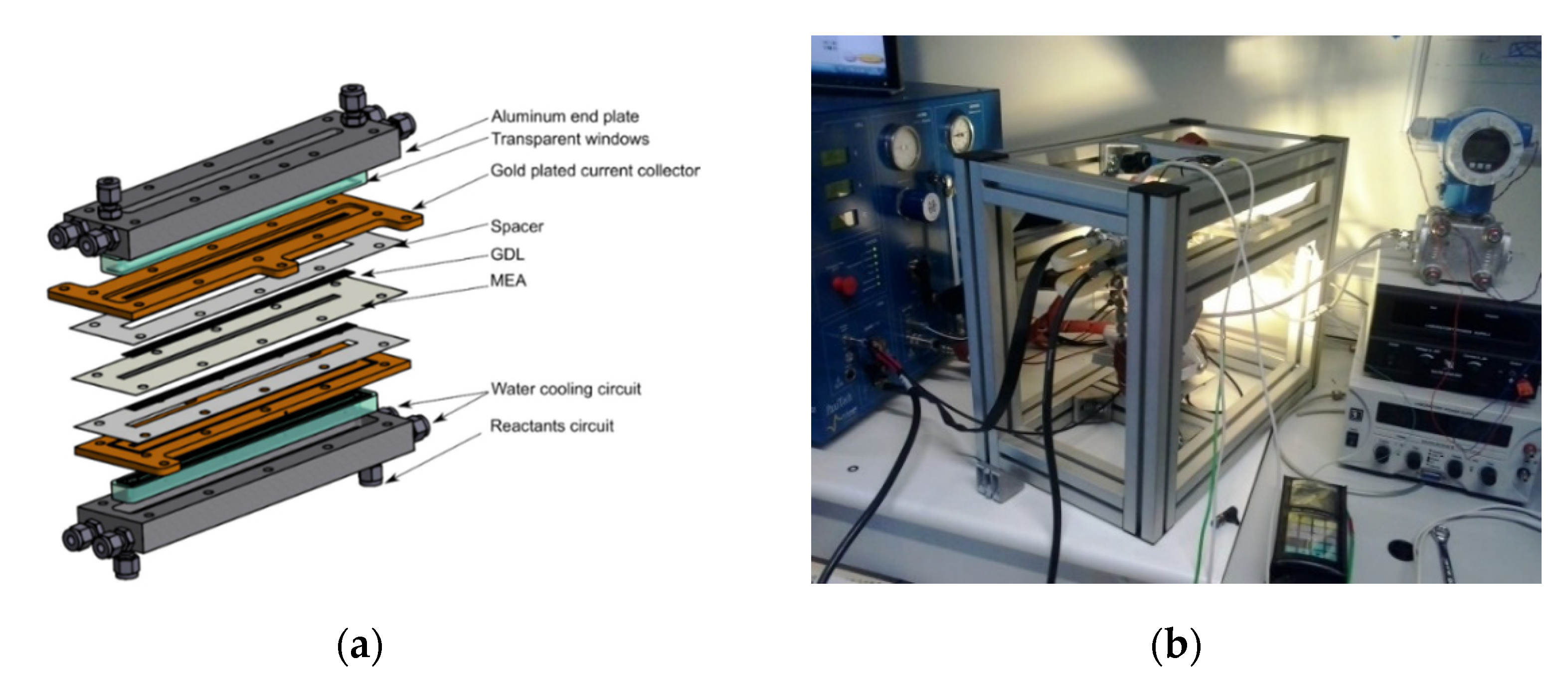
A half-cell including a straight channel, a porous gas diffusion layer (GDL), and a catalyst layer (CL) is considered. A cross-section of this cell is given in Figure 1a. Oxygen transport is considered through the electrode and GDL. Only cathode electrochemical transfers are modeled. The anode is not considered in the model due to much faster kinetic reaction compared to those occurring on the cathode side. Liquid water has not been considered in the model. Figure 1b shows a simple fuel cell electrical circuit.
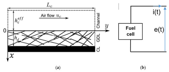
Figure 1.
(a) PEMFC half-cell geometry reprinted from [28]. (b) A simple fuel cell electrical circuit.
The model is based on the following assumptions:
- Oxygen transport in the cathode catalyst layer (CCL) is fast;
- The oxygen transport in the GDL is purely 1D in the x-direction;
- The oxygen transport in the channel is assumed to be a plug-flow with an averaged velocity and the choice of plug flow in fuel cell microchannels is justified by the small dimensions of the channels. It was shown in previous studies [29,30] that the laminar velocity profile in rectangular microchannels is flat at the center. Thus, at the first order and given the high mass diffusivity of air in the cathode channel, one can assume that the average velocity of a plug flow is able to give a good description of the mass transfer in the fuel cell microchannels;
- The model is isothermal;
- The CL is supposed to be infinitely small;
- The voltage potential is equal along the CL in the y-dimension;
- All channels of the cell are supposed to be operated in the same condition such as temperature, humidity, etc.; and
- The concentrations in the canal and the GDL are supposed to be equal (concentration on the channel inlet) before any current is applied to the FC.
2.2. General Equations
The first equation is the one describing the physical model in the channel and the oxygen transport. This equation is represented by the local continuity equation [31]:
with
Equation (1b) represents the boundary conditions at the channel entry. In the GDL, the oxygen transport is described by the first and second Fick’s law as in [31]:
with
The instantaneous current density produced by a fuel cell can be written as the sum of a faradaic (derived from Tafel law) and a capacitive current density [31]:
with
The boundary conditions at the GDL/CL interface are described by
The fuel cell voltage satisfies [31]:
The fuel cell current can be computed using
In this section, a 2D physical model of the fuel cell has been presented. In the next section, the system of equations is transformed into dimensionless coordinates. The model is then spatially discretized in Section 3 using a finite difference technique. To validate the proposed model, simulations are performed using the Matlab/Simulink environment and compared to experimental data, as detailed in Section 5.
2.3. Normalized Adimensional Equations
For the transformation to dimensionless coordinates, the following normalized variables are used [28]:
Appendix A shows the value of and .
The physical model of Equations (1)–(5) are rewritten in dimensionless coordinates. In the channel, the oxygen transport equation and the boundary conditions become
In the GDL, the oxygen transport equation is rewritten as
In the CL, the normalized current density represented by Equation (3a) becomes
The fuel cell voltage can be represented as
The boundary conditions equation at CL/GDL can be rewritten as
The cell current density is calculated by
The current density in Equation (12a) is replaced by that in Equation (9) to give the potential Equation (12b).
3. Finite-Difference Discretization
To numerically solve the mathematical model represented by Equations (7)–(12) with known boundary conditions, a finite-difference discretization technique is used in this paper. For the channel and the GDL, a spatial meshing with discretization steps , is considered. The discretization uses central differences when possible and forward or backward differences when not. It is formulated as:
with
Equations (7) and (8) can be rewritten using Equation (13a–d).
In the canal, the equations can be written as:
= 0, Equation (1b) is used.
In the GDL, we can write:
Equation (13d) is used.
In the Catalyst Layer (CL), the potential can be computed as
Finally, for , the current density is calculated from Equation (13f). The fuel cell current represented in Equation (5) can be calculated by
4. Description of the Experimental Test Bench and Considered Fuel Cell
A 12 cm2 single cell was specially designed to validate the proposed model. It includes two parallel channels of 1.5 width and in length. The flow field was machined directly in the copper current collector to enable an optical access inside the channel via a transparent Plexiglas plate on the top of the channel (see Figure 2). The current collectors were also gold-plated to ensure minimal ohmic resistance. Between the current collector, a membrane electrode assembly (MEA) was inserted; it was made of a thick Gore PEM with platinum loading in the CL. The thin membrane and high platinum loading were specially chosen to ensure low membrane resistance and high current density. The MEA was sandwiched between two 10BC GDL from SGL® compressed to a width of using two rigid spacers. Finally, two aluminum end-plates were used to assemble all the fuel cell components. A water-cooling circuit connected to a temperature control system was drilled inside the endplates to keep the fuel cell temperature constant.

Figure 2.
(a) Three-dimensional view of the straight channel fuel cell reprinted from [32]. (b) Fuel cell benchmark setup in LTeN, Nantes.
The fuel cell was connected to a FCT 50 test station from BioLogic® to control the air and hydrogen flow rates, temperatures, humidity, and pressure. The current and voltage were also recorded through the FCT 50 test station.
5. Experimental Validation of PEMFC Model
Reliable voltage/current curves require a stable environment where the temperature, pressure, humidity, and flow rates are kept constant while the tests are being conducted. If the conditions are fluctuating, the voltage/current characteristics may change. In addition to keeping the testing environment stable, a second consideration is the condition of the fuel cell itself which can take time to stabilize. Depending upon the fuel cell design and size, this stabilization phase may take up to 30 min following a change in current or voltage. All measurements were conducted using the parameters listed in Table 2 and under a constant stoichiometric ratio of H2 (1.1) and air (5), with a relative humidity of 15%.
Table 2.
PEMFC model parameter values.
Using Equations (14) and (15), a PEMFC model was built with the MATLAB/SIMULINK environment. To compare the experimental and simulated results, several tests were carried out. The specifications of the PC used for these calculations are Intel Core i7-3770 CPU and 3.4 GHz with 16 GB RAM.
5.1. Current Profile with Step-Up
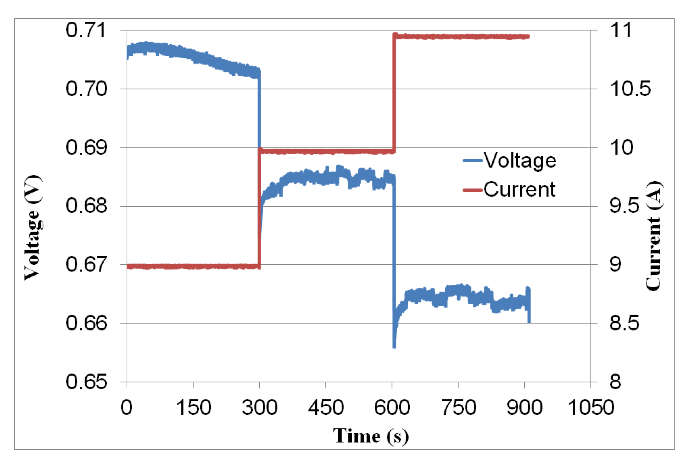
To validate our PEMFC model around the nominal operating point (), a piecewise constant current was applied. Figure 3 shows the dynamic response of voltage with different current levels of , and .
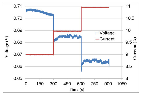
Figure 3.
Experimental current and voltage of fuel cell.
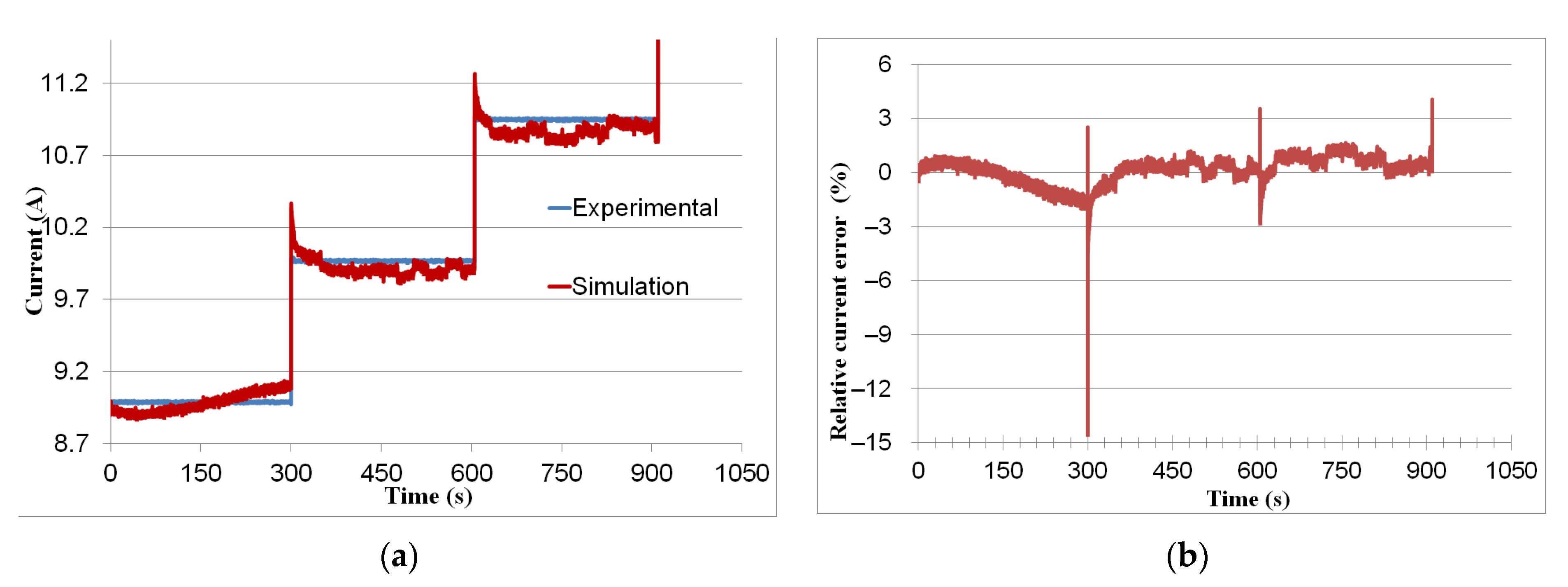
The fuel cell measurements presented in Figure 3 were obtained after an extended period of operation. The voltage variation shown here indicates that when the current steps up to a higher value, the voltage can undergo three changes: an instantaneous drop due to the set of ohmic resistances (electrodes, membrane, bipolar plates, etc.) [33], a quick recovery because the cell takes several seconds for the back-diffusion water to re-wet the anode side so as to ease water redistribution and recover the cell performance [11], and a slow increase due to changes in membrane resistance. Figure 4 compares the simulation and experimental results for the fuel cell current. The relative current error oscillates around zero with a mean value of 1.7%, as shown in Figure 4b.
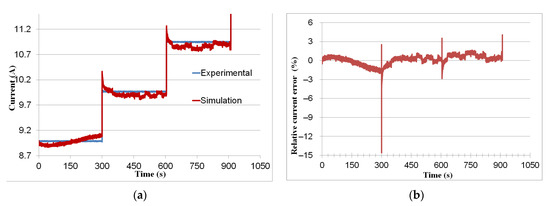
Figure 4.
(a) Simulation and experimental curves of current. (b) Relative error of simulated current.
5.2. Current Profile with Forward/Backward Sweeps
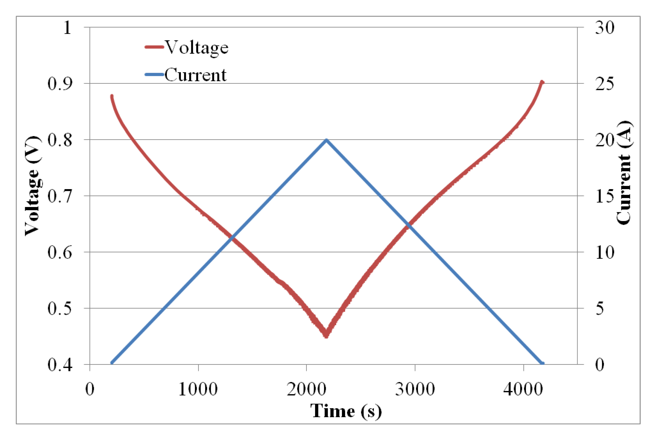
The fuel cell was swept with a current rate of , from to (forward sweep) and back to (back sweep). The measurements of the current and voltage are shown in Figure 5. The voltage gradually decreased from the open-circuit voltage to a low value.
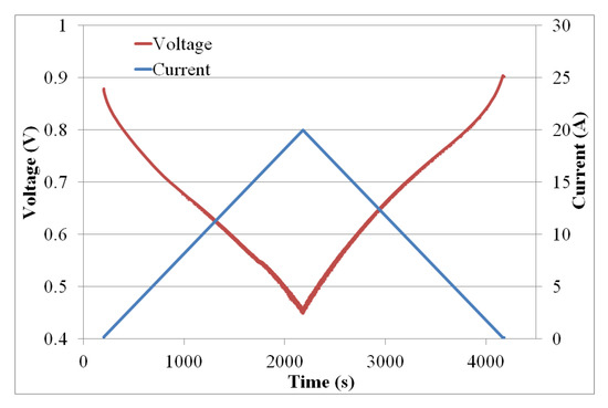
Figure 5.
Experimental current and voltage of PEMFC for forward/backward sweep.
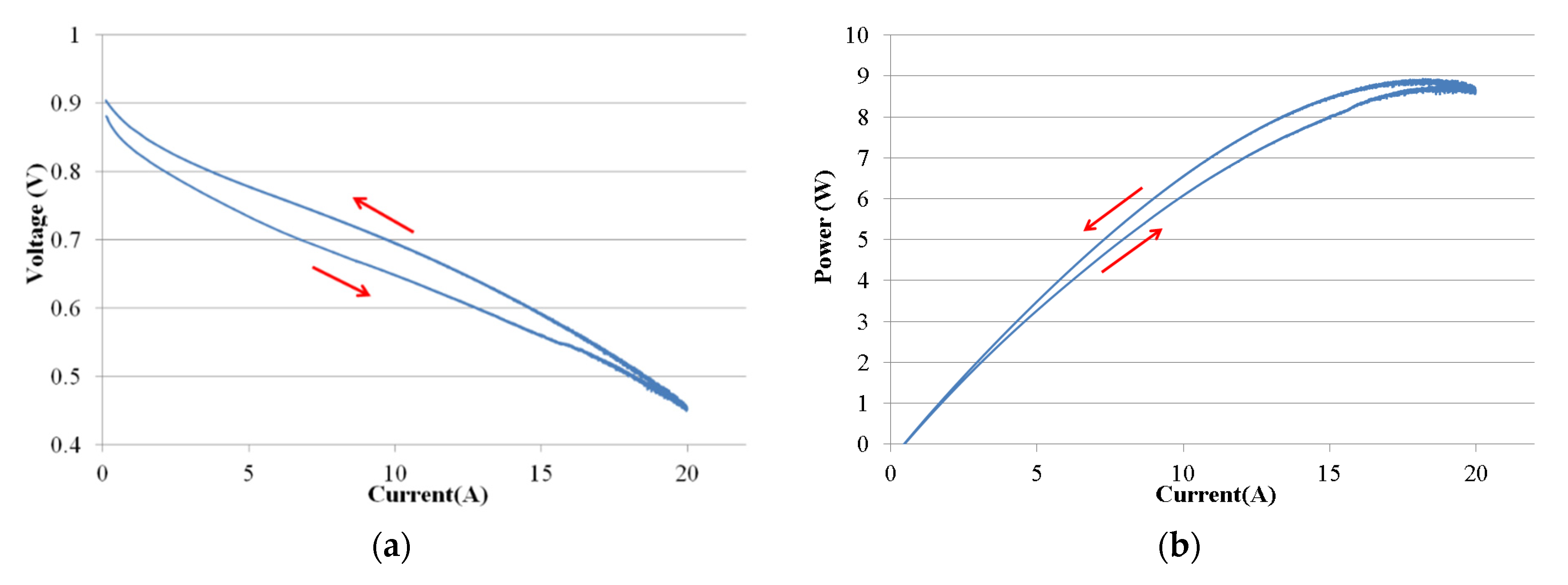
The polarization curve is useful for troubleshooting issues in the fuel cell stack. If the polarization curve is recorded while increasing and decreasing the current, it may show hysteresis. This typically indicates a change in fuel cell conditions, such as drying or flooding of the membrane. Figure 6a represents the voltage of the fuel cell as a function of the current. It was observed that the voltage under the forward sweep is lower than that under the backward sweep. Figure 6b shows the output cell power vs. the current, where the power increases with the increase in current. The power reaches the maximum power point for a current of 18 A and then it decreases [34].
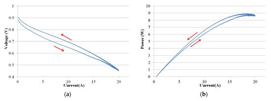
Figure 6.
(a) Experimental V/I characteristic for the studied PEMFC. (b) PEMFC power vs. current.
This improved performance during the backward sweep compared with the forward sweep can be explained by the variation of hydration levels in the membrane because the humidity level in the membrane directly influences its conductivity. When the current increases, more water vapor is produced, causing an increase of the internal conductivity. During backward swapping, the membrane was still saturated or at high humidity levels, thus it exhibited an improved performance. In addition, the difference between the forward and backward voltage at a lower current range is more important than at the higher current range. This is due to the increased water content observed in our electrolyte results caused by the increased electrode kinetics.
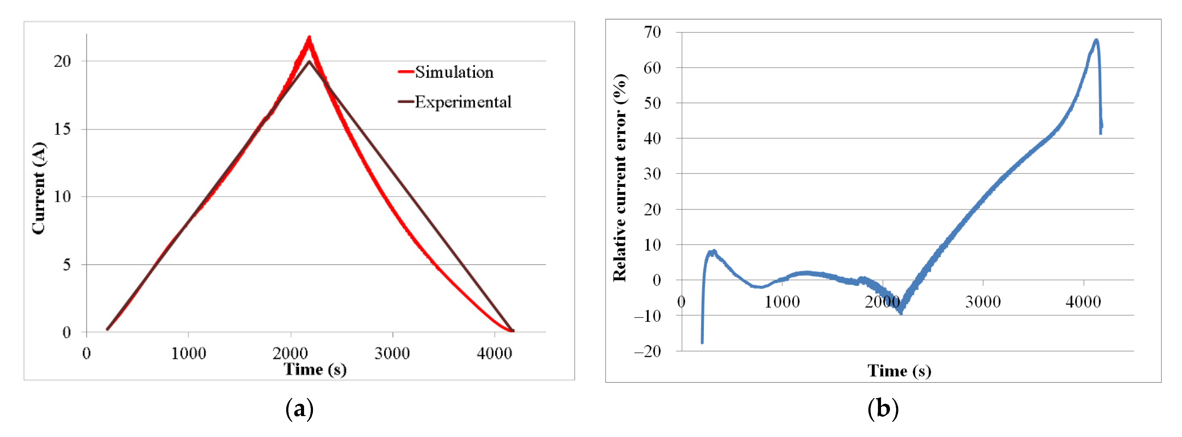
The PEMFC model was implemented in the Matlab/Simulink environment and was designed with voltage input and current output. Equation (14a–d) were solved with the ODE45 Dormand-Prince variable-step differential equation solver, which is considered to be one of the best methods for treating non-stiff general-form initial value problems for ODE. The current density of the fuel cell was then computed using Equation (13f). The total fuel cell current was obtained from Equation (15). The simulated and experimental currents are shown in Figure 7a. The simulation was conducted with different discretization steps, where various grid sizes (K, D) were used as this was expected to have a negligible impact on the accuracy. Sweeping the fuel cells at different current levels highlighted several phenomena. When the current exceeds 15 A, the voltage is distorted (Figure 5) and the error between the simulation and experimental currents becomes more important (Figure 7b). For the backward sweep, the relative current error increases linearly.
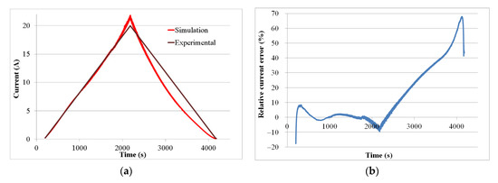
Figure 7.
(a) Simulation and experimental curves of current. (b) Relative error of simulated current.
6. Estimating the PEMFC Parameters Using an Extended Kalman Filter
The voltage and current are considered as the input–output model. To design the observer, we used the continuous-discrete extended Kalman filter (CD-EKF) [35]. This technique uses a numerical integration of the ordinary differential equations to predict the state of the continuous-time dynamic system and the corresponding prediction error covariance matrix. A standard discrete-time correction step of the extended Kalman filter (EKF) is then applied to arrive at a more accurate state estimation. The state variables vector was chosen as:
where goes from 1 to for and from 0 to for , and. goes from to (for . For = is determined by the boundary condition (Equation (1b)). For = is calculated from the boundary condition (Equation (13d)). Thus, we have state variables. The state equations for the concentration in the channel () and GDL (), and potential () were described previously (Equation (14)). The time derivatives of , , , , and are considered equal to zero. The system of interest is a continuous-time dynamic system with a discrete-time measurement given by [36,37,38]:
where is the unmeasured “process noise” which is assumed to be a continuous-time zero-mean white noise of covariance and is measurement noise covariance. is the measurement noise which is assumed to be discrete-time white noise with zero mean, with The Kalman Filter mainly involves two steps: prediction and measurement update. The predicted state and its covariance are calculated by solving Ordinary Differential Equations (ODE) [39]:
The dynamic matrix (the Jacobian matrix of the partial derivatives of function ) is computed as follows:
The matrix parts (Equation (19)) are given in Appendix B. The equations used to calculate the different terms in the Jacobian matrix are also given in Appendix C.
The two parts of Equation (18) can be solved simultaneously with an ODE solver [40]. Equation (18b) is vectorized. Here, the filter (CD-EKF) is simulated in Matlab/Simulink with ODE45. The integration is done in the interval with the initial conditions and error covariance matrix . The predicted state and the error covariance matrix at the time point are computed. Then, the standard correction step of the EKF is used. Additionally, only the upper triangular part of the error covariance matrix, including the main diagonal because of its symmetry, is calculated. The standard measurement update is applied at the time (). The observation function can be deduced from Equations (15) and (13f) as:
Supposing the constant , we can rewrite Equation (20a) as a function of the state variables as
The observation matrix can be calculated by
where
The Kalman gain can be computed as:
As presented in [41], Auger et al. proposed that the value of covariance can be set to one (). The state estimate covariance is updated by the equation:
We use the Kalman gain to update the state estimate:
Lastly, the calculation process repeats itself. The proposed EKF requires a high computation effort and is not appropriate for online estimation of PEMFC parameters. Hence, some simplifications have been implemented to calculate the covariance matrix of the predicted state (Equation (18b)) using Mazzoni’s formulae [42]. Mazzoni’s formulae, which are based on the implicit midpoint method, are rearranged as follows:
where is the identity matrix of size . Due to the application of the simplification method, it is expected that the model accuracy will be decreased, albeit the model-solving is faster [43].
7. Results of the EKF Observer and Discussion
7.1. Current Profile with Forward/Backward Sweeps
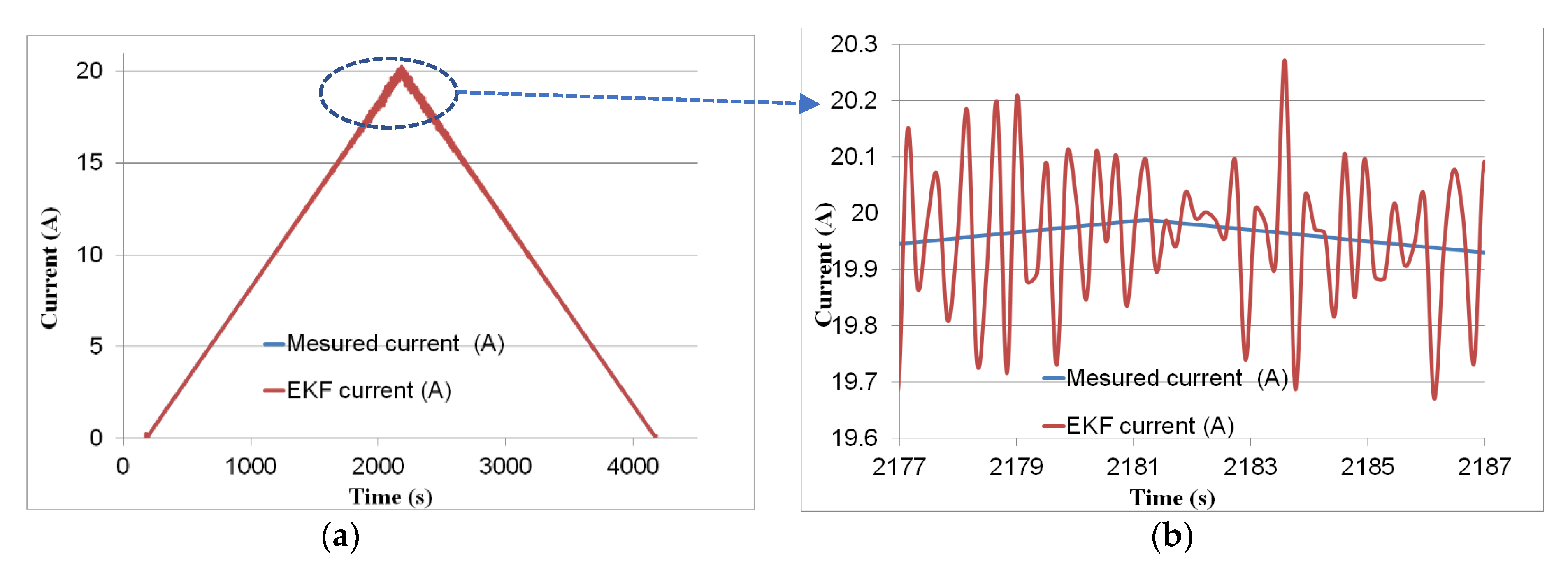
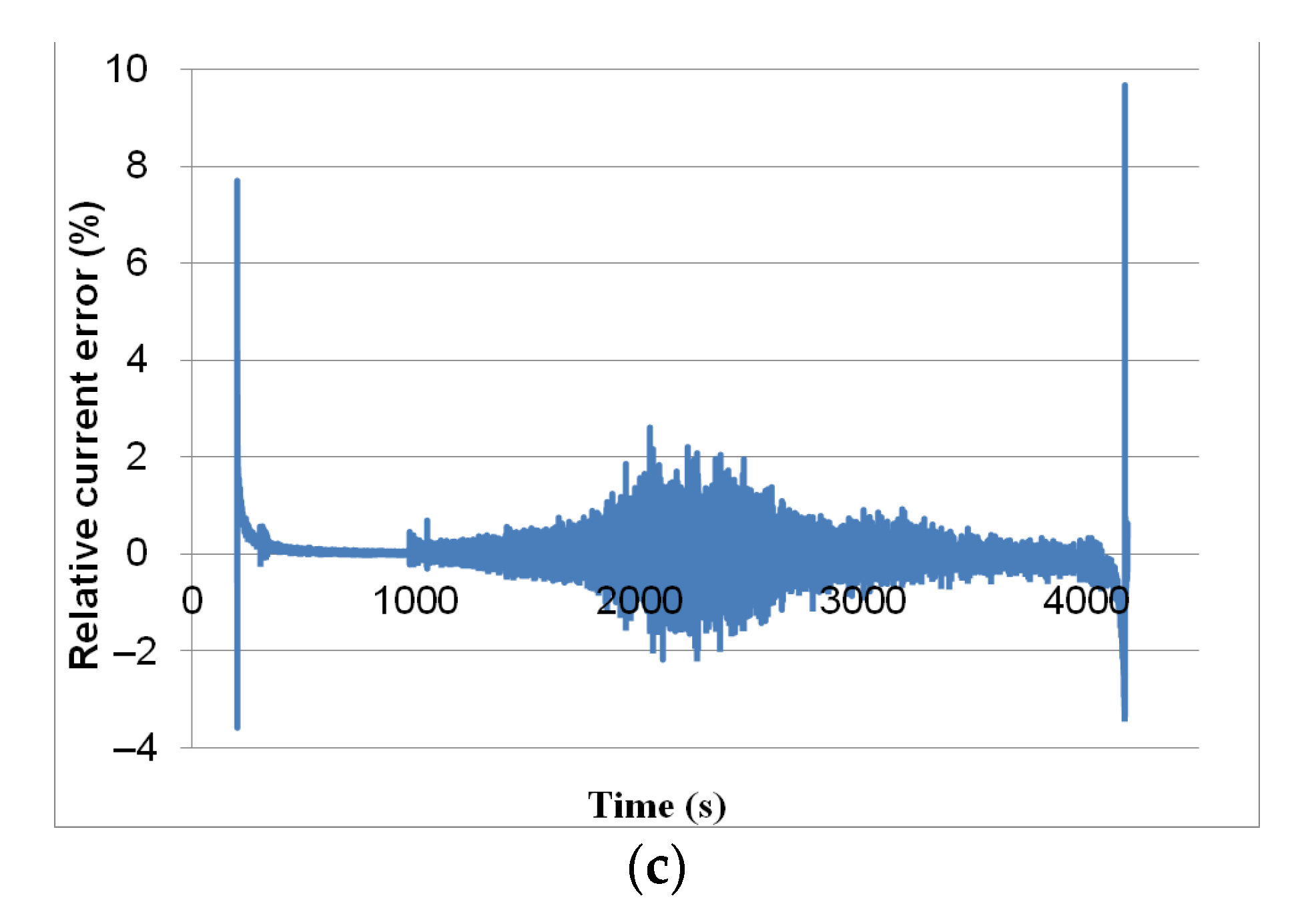
To ensure that all results obtained in this study are not overly sensitive to the fineness of the spatial discretization, a mesh sensitivity analysis was performed. The values of and were optimized by simulation. To validate the EKF observer designed for and , the same voltage/current measurements shown previously in Figure 5 were used. The PEMFC current measured experimentally was compared to the current estimated by the EKF (. The current estimated by EKF converged well with the experimental data, as shown in Figure 8a. Figure 8b shows a zoomed-in image of both curves between 2177 s and 2187 s; it confirms the estimated current’s convergence with the experimental current. Except at the beginning and end of the curve (where the PEMFC current is of the order of a few mA), the relative error is quite low, as shown in Figure 8c, with a mean value of As shown in Figure 7a, there is a significant error between the experimental data and the output of the model simulated using time-invariant parameters. This error becomes negligible when using time-varying parameters estimated by a continuous-discrete EKF, as illustrated in Figure 8a.
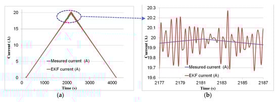

Figure 8.
(a) Measured current and current estimated by EKF. (b) Zoomed-in image of both curves between 2177 and 2187 s. (c) Relative error of estimated current.
Ambient air was employed as the oxygen source at the cathode, oxygen was consumed by the reaction at CL, and the concentration of oxygen was reduced between the inlet and outlet of the gas flow channel. When the FC current is higher, the electrochemical reaction becomes stronger and more oxygen is consumed at CL, leading to lower oxygen concentration inside the GDL. The variation of the oxygen concentrations in the channel is presented in Figure 9a as a function of time and . This concentration strongly depended on the current value (see Figure 8a). As an example, for , this concentration decreased with time until the minimum value was reached at time s for a current of 20 A. Diffusion across the cathode GDL is caused by a concentration differential between the gas flow channel and the CL. The variation of concentration as a function of time and for two values of (,) is presented in Figure 9b. Following this graph, it can be seen that the concentration values decrease with time as a result of the current variation, especially for the highest value of . For , for example, the concentration decreased over time until it reached its minimum value at time s for a current of 20 A.
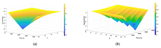
Figure 9.
(a) Concentration as a function of time and . (b) Concentration as a function of time and , and two values of = and.
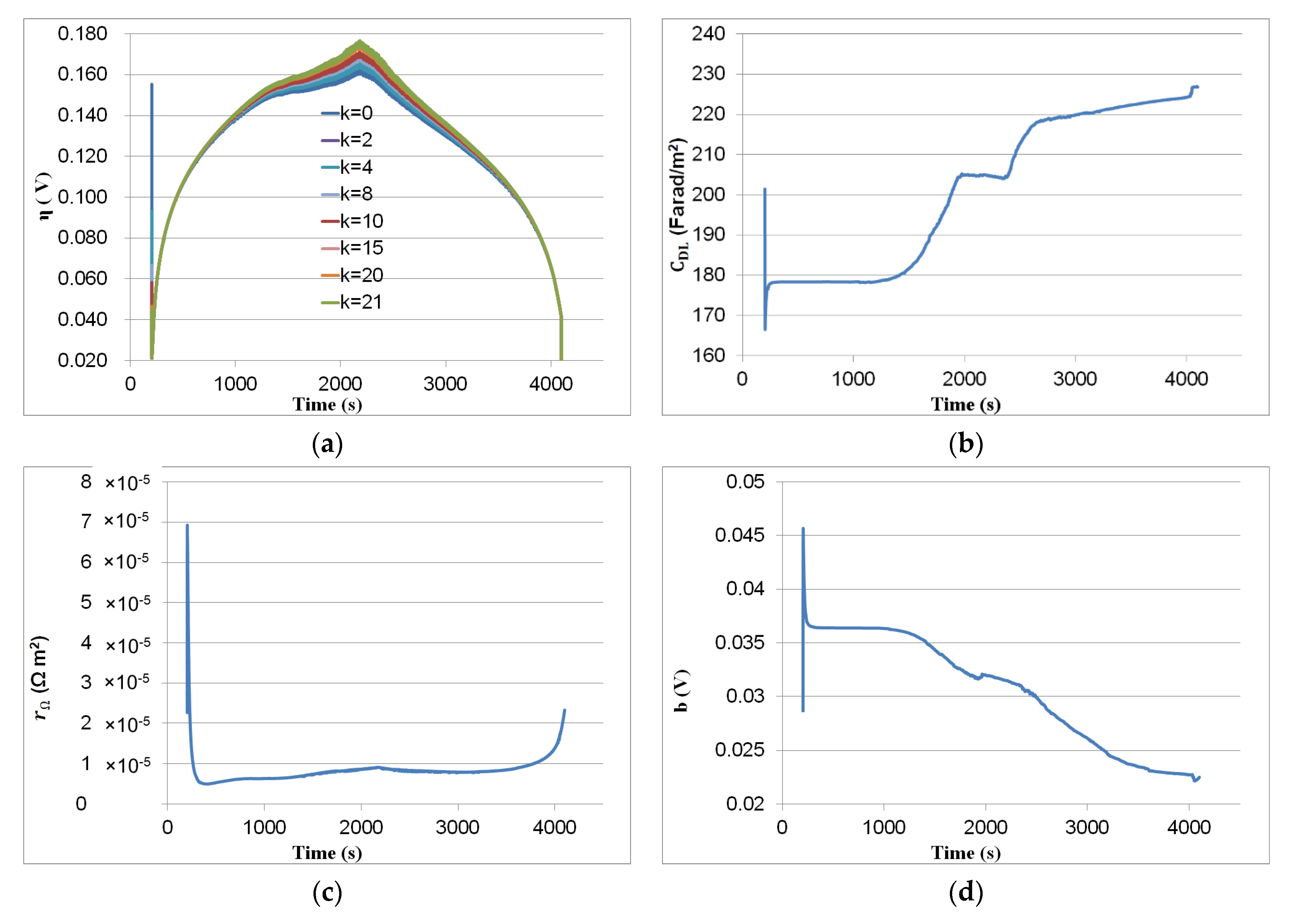
Figure 10 shows the variation of the estimated parameters with time. Figure 10a shows the variation of potential as a function of time for different values of . The value of potential follows the PEMFC current values. The hysteresis phenomena can be observed on the potential curve for the forward/backward sweep. As illustrated in Figure 10b, the capacitances vary slightly. As presented in Figure 10c, the estimated resistance increased hardly for the forward sweep and for the backward sweep, it was still constant. This could be attributed to the FC’s temperature as well as to hydration. A proper water content in a fuel cell will reduce the membrane resistance and promote the electrochemical reaction in the cell [44]. Tafel slope represents the voltage losses due to activation polarization. It depends on current [31], humidity, and operating temperature [45]. The Tafel slope decreased lightly, as depicted in Figure 10d. As shown in [31], this variation is fairly small because can fluctuate from to as a function of various operating conditions [31]. The diffusion coefficient was slightly variable within the backward sweep (Figure 10f). The results explained in [46] show that the through-plane gas diffusion coefficient decreases as the number of hydrophilic pores in the GDL increase due to blocking of pores by liquid water. The exchange current density depends on the roughness of the electrode surface; its catalytic properties; the presence of oxides and water; the concentration of the reactive species; the composition of the electrode and electrolyte; and the temperature [47]. As can be seen in Figure 10e, the exchange current density increased greatly. The exchange current density increases with the increase of temperature [48]. The exchange current density has three phases: a constant between 0 s and 1200 s because the current is low (the temperature is close to the starting temperature); an exponential increase between 1200 s and 2100 s, where the current rises and the internal temperature rises with it; and a second exponential increase between 2100 s and 4000 s.
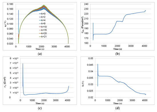
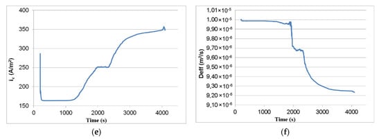
Figure 10.
EKF results: (a) potential ; (b) capacitances ; (c) resistance ; (d) Tafel slope ; (e) exchange current density ; and (f) diffusion coefficient .
7.2. Current Profile with Step-Up/Down
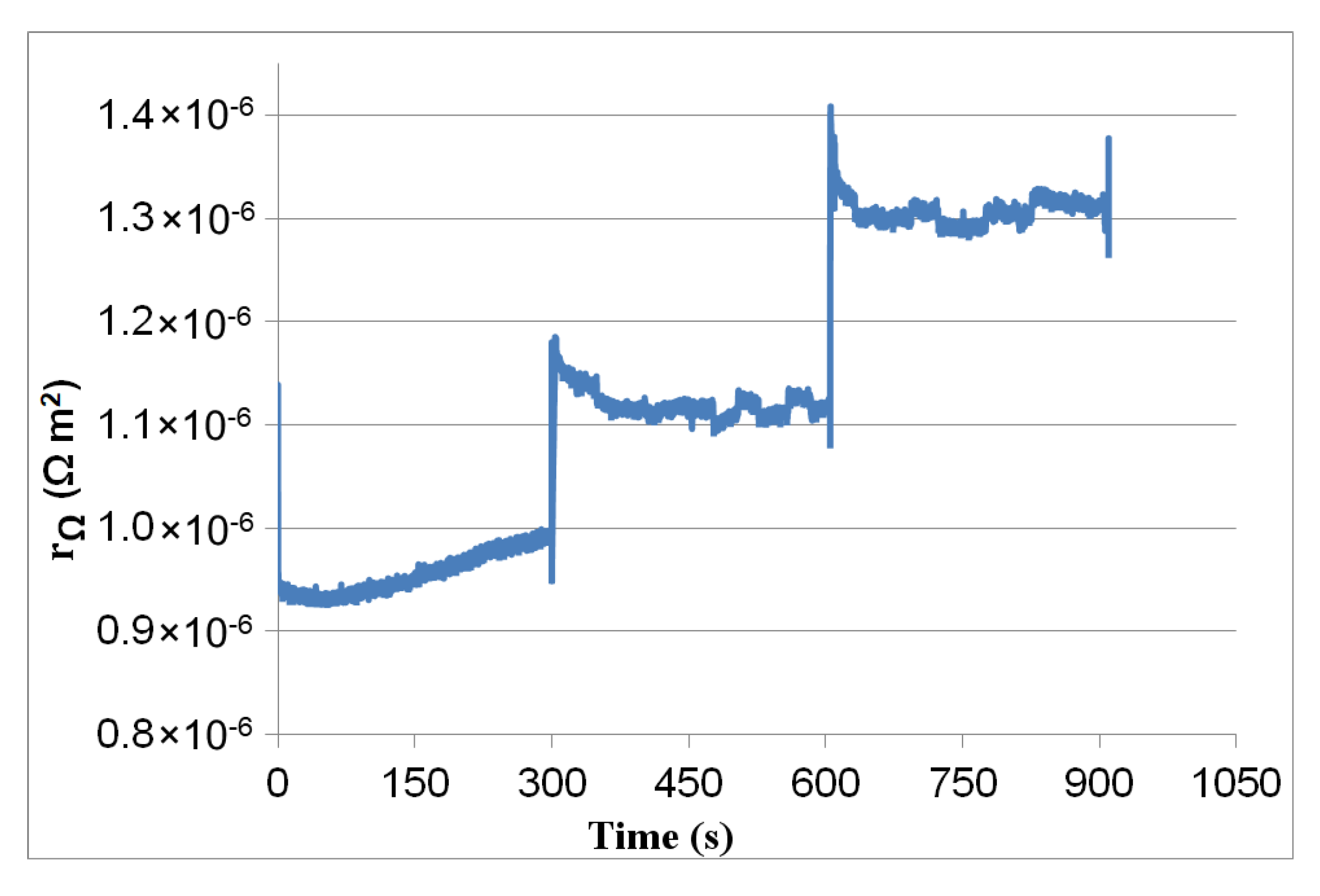
The EKF observer was applied with the same initial parameters as in the section above and for the experimental results presented in Figure 3. The Tafel slope , capacitance , and current were slightly variable for this short simulation period. The potential value , as well as the and concentrations, were heavily influenced by the PEMFC current levels. The resistance estimated by EKF is represented in Figure 11.
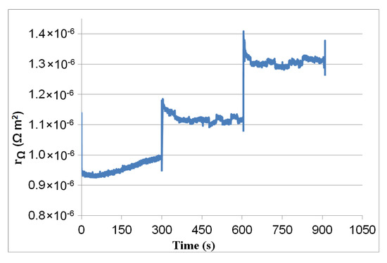
Figure 11.
Estimated resistance .
Figure 11 shows how the sharp voltage drops at t = 300 s and 600 s (see Figure 3) because of inevitable jumps in the membrane resistance. Then, the resistance decreases or increases slowly according to voltage variation. The flooding effect may cause transient fluctuations in membrane resistance, as seen in Figure 11 after a long course of running. Reference [49] explains the relationship between current density, membrane resistance, and water content. A positive feedback loop exists between current density, which produces water, and membrane resistancewhich increases with water contentas the water content increases. However, the membrane resistance is typically a small component of the overall cell resistance. For the feedback mechanism to destabilize the cell and generate hysteresis, the membrane resistance must be particularly sensitive to water content.
7.3. Modified PEMFC Cell with Step-Up/Down Profile
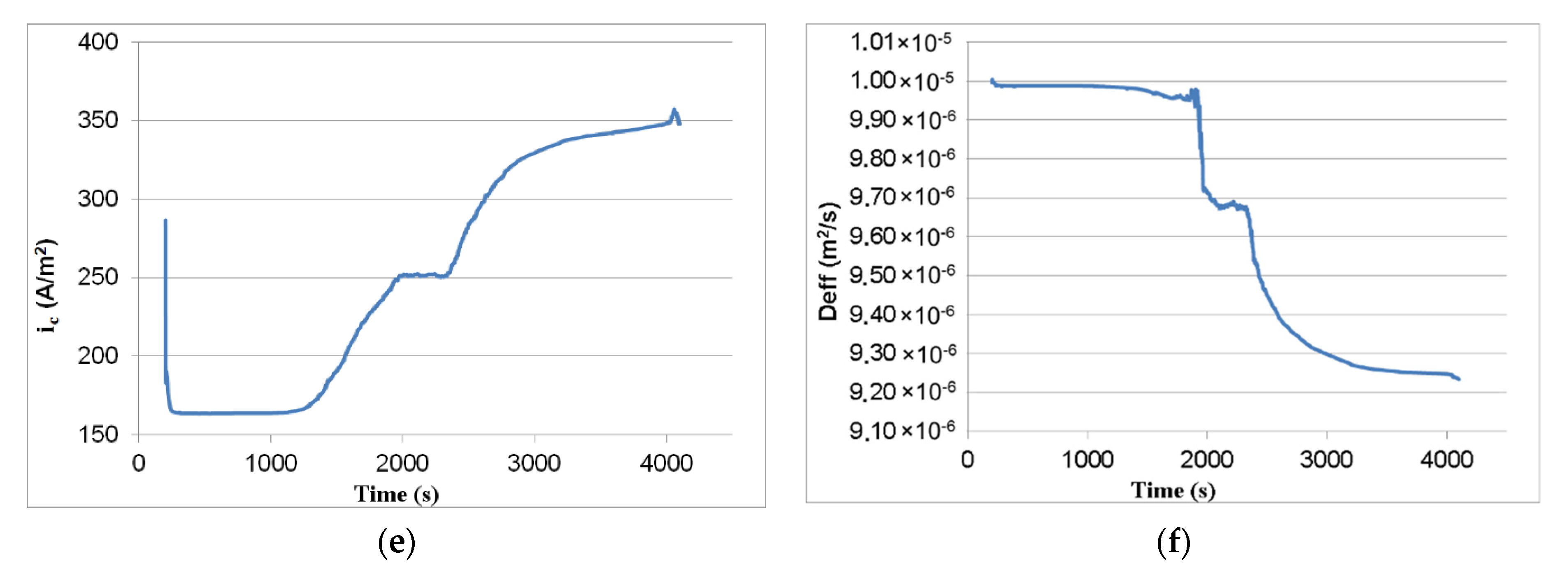
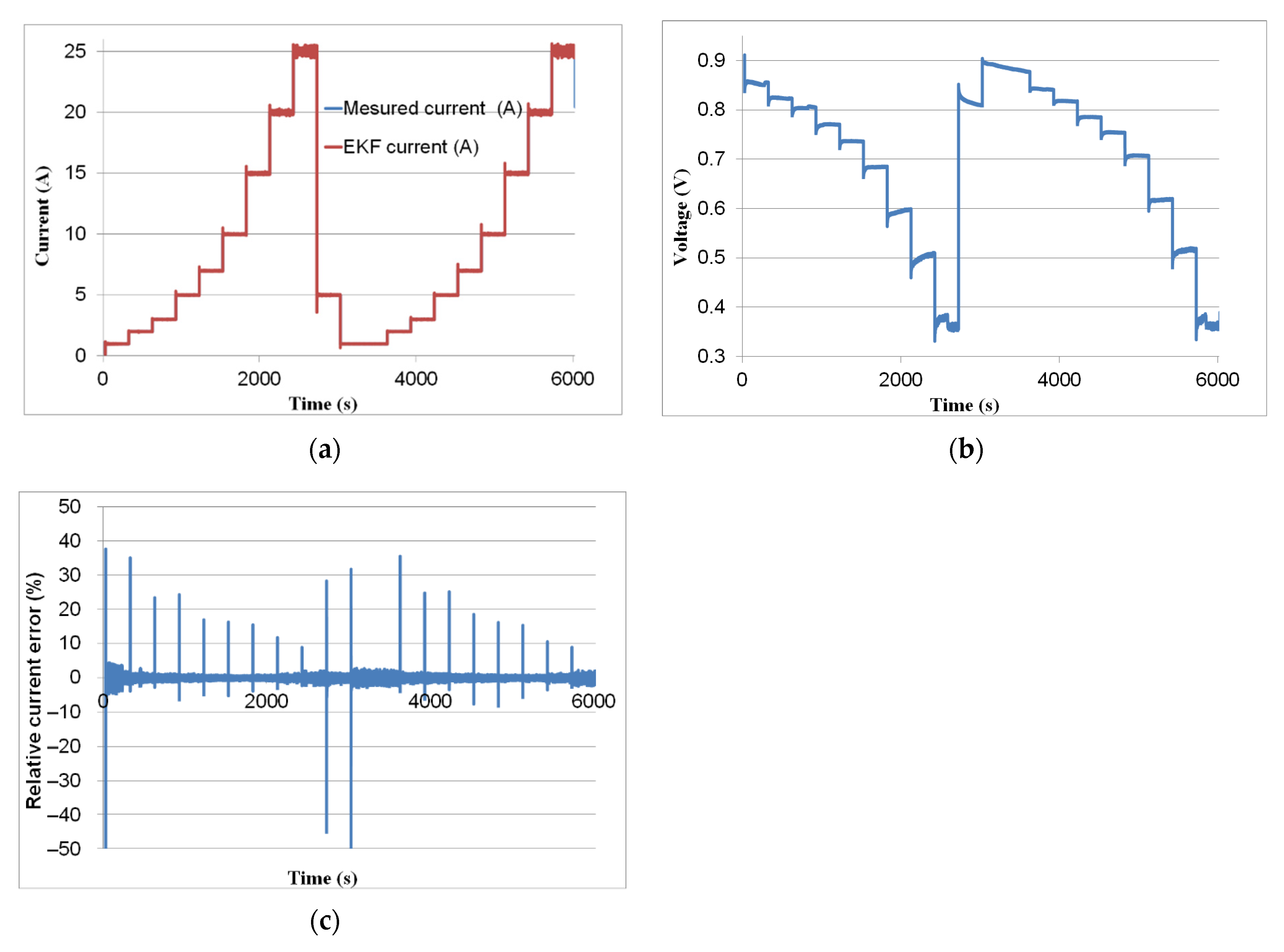
We used the same fuel cell mentioned previously but its channel width was changed from to . The current and voltage profiles with step-up/down were conducted as shown in Figure 12a,b. The current consisted of two step-up cycles (0 to 25 A) interspersed with a hard drop from 25 A to 5 A and then to 1 A, while the voltage varied in a range of 0.3 to 0.9 V (Figure 12b). This current/voltage profile can span the whole operating area of the investigated FC. It enables large changes in the parameters of the FC model. The EKF estimated and experimental currents are compared in Figure 12a. The relative current error is illustrated in Figure 12c. Its value is lower than 0.035% but takes a higher value when the current steps up or steps down.
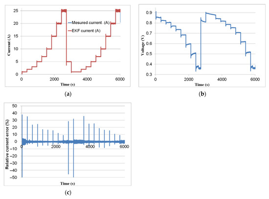
Figure 12.
(a) Measured current and current estimated by EKF. (b) Experimental voltage of a new PEMFC cell for step-up/down profile. (c) Relative error of the estimated current.
Figure 13 shows the parameters estimated with EKF vs. time. Figure 13a shows the variation of potential with time. The current value substantially influences the potential . As shown in Figure 13a, its variation was similar to the current one. As explained in [11], when the current drops from a high value to zero or a low value, the double-layer charge effect can appear. Figure 13b illustrates that despite the large current variation, the value of the double-layer capacitor dod not vary. Due to the low hydration and temperature at a low current, the resistance began with a high value and then gradually declined, as seen in Figure 13c. The resistance decreases with the increase in humidity, current, and temperature [50,51,52]. The Tafel slope increased with time, as indicated in Figure 13d. The rise in could be attributable to an increase in temperatures and decreasing pore porosity, which decreases as humidity rises. The exchange current density vs. time is depicted in Figure 13e. The exchange current took a higher value compared with previous cases (Figure 10e). As depicted in Figure 13f, the diffusion coefficient increased from to . The increase in could be due to an increase in temperature. When the current dropped from to , the diffusion coefficient jumped downward, as illustrated in Figure 13f. The effective diffusion coefficient decreases as the number of hydrophilic pores increases because liquid water blocks the pores in the GDL [46].
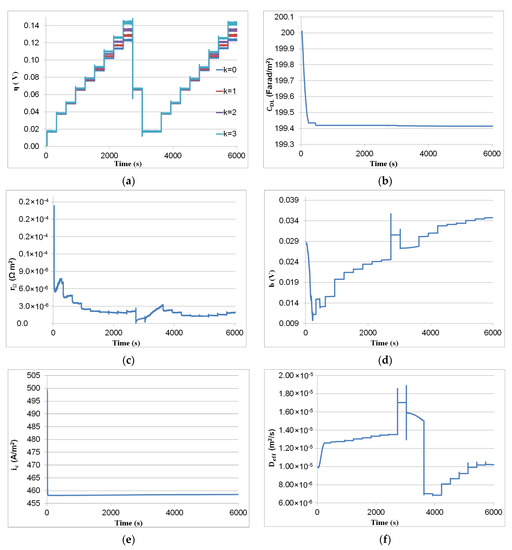
Figure 13.
EKF results: (a) potential ; (b) capacitances ; (c) resistance ; (d) Tafel slope ; (e) exchange current density ; and (f) diffusion coefficient .
Table 3 summarizes the observer performances in terms of processing for the current profiles presented in Section 7.1 and Section 7.3. The EKF simulation with the data considered in Section 7.1 lasted 2340 s, which is substantially less than the duration of the real-time measurement (3779 s). The EKF simulation with data in Section 7.3 lasted 5188 s against 6000 s for the period of the real-time measurement. This means that the EKF can estimate the PEMFC parameters before the time period between two samples elapsed. In addition, these simulations demonstrate that despite the enormous number of state variables (n = 340), the observer was able to estimate the PEMFC parameters faster than the real-time measurement.
Table 3.
EKF results.
8. Conclusions
In this paper, the design of a 2D physics-based diagnostic model for the PEMFC is presented. The model is extracted from Fick’s laws and Tafel’s equation, which relate to the oxygen transport in fuel cell channels and the gas-diffusion layer (GDL). The proposed PEMFC model is spatially discretized and using this discretized PEMFC model, a continuous-discrete extended Kalman filter was designed. Mazzoni’s formulae are later applied on the EKF to accelerate the calculation time of the PEMFC state observer.
For various current profiles, the EKF was used to estimate the PEMFC parameters. This observer accurately estimates the PEMFC’s dynamic ohmic resistance considering the load variation. The most important characteristic of the observer is its capability to estimate the PEMFC parameters in real-time.
Other operating conditions affect the PEMFC, such as aging and the membrane state (dry, wet, and flooded). In addition, the ohmic resistance of the PEMFC depends on the aging of the PEMFC and, consequently, the SoH of the PEMFC affects its ohmic resistance. In future work, the PEMFC observer can be extended to estimate both lifetime and aging.
Author Contributions
Conceptualization: Y.D., F.A, E.S. and S.C. methodology: Y.D., F.A, E.S. and S.C; software: Y.D. and F.A; writing—original draft: Y.D., F.A. and S.C.; writing—review and editing: Y.D., F.A., S.C. and A.A. All authors have read and agreed to the published version of the manuscript.
Funding
This research received no external funding.
Institutional Review Board Statement
Not applicable.
Informed Consent Statement
Not applicable.
Data Availability Statement
Not applicable.
Conflicts of Interest
The authors declare no conflict of interest.
Appendix A
Appendix B
Appendix C
References
- Du, Z.; Liu, C.; Zhai, J.; Guo, X.; Xiong, Y.; Su, W.; He, G. A Review of Hydrogen Purification Technologies for Fuel Cell Vehicles. Catalysts 2021, 11, 393. [Google Scholar] [CrossRef]
- Madsen, R.T.; Klebanoff, L.E.; Caughlan, S.A.M.; Pratt, J.W.; Leach, T.S.; Appelgate Jr, T.B.; Kelety, S.Z.; Wintervoll, H.-C.; Haugom, G.P.; Teo, A.T.Y. Feasibility of the Zero-V: A Zero-Emissions Hydrogen Fuel-Cell Coastal Research Vessel. Int. J. Hydrogen Energy 2020, 45, 25328–25343. [Google Scholar] [CrossRef]
- Klebanoff, L.; Pratt, J.; Johnson, T.; Arienti, M.; Shaw, L.; Moreno, M. Analysis of H2 Storage Needs for Early Market Non-Motive Fuel Cell Applications; Technical Report SAND2012-17392012; Sandia National Laboratories: Livermore, CA, USA, 2012. [Google Scholar]
- Ursua, A.; Gandia, L.M.; Sanchis, P. Hydrogen Production from Water Electrolysis: Current Status and Future Trends. Proc. IEEE 2012, 100, 410–426. [Google Scholar] [CrossRef]
- Gray, E.M.; Webb, C.J.; Andrews, J.; Shabani, B.; Tsai, P.J.; Chan, S.L.I. Hydrogen Storage for Off-Grid Power Supply. Int. J. Hydrogen Energy 2011, 36, 654–663. [Google Scholar] [CrossRef]
- Petrovic, S.; Hossain, E. Development of a Novel Technological Readiness Assessment Tool for Fuel Cell Technology. IEEE Access 2020, 8, 132237–132252. [Google Scholar] [CrossRef]
- Larminie, J.; Dicks, A.; McDonald, M.S. Fuel Cell Systems Explained; J. Wiley: Chichester, UK, 2003; Volume 2. [Google Scholar]
- Zhong, Z.-D.; Zhu, X.-J.; Cao, G.-Y.; Shi, J.-H. A Hybrid Multi-Variable Experimental Model for a PEMFC. J. Power Source 2007, 164, 746–751. [Google Scholar] [CrossRef]
- Zhong, Z.-D.; Zhu, X.-J.; Cao, G.-Y. Modeling a PEMFC by a Support Vector Machine. J. Power Source 2006, 160, 293–298. [Google Scholar] [CrossRef]
- Husar, A.; Strahl, S.; Riera, J. Experimental Characterization Methodology for the Identification of Voltage Losses of PEMFC: Applied to an Open Cathode Stack. Int. J. Hydrogen Energy 2012, 37, 7309–7315. [Google Scholar] [CrossRef] [Green Version]
- Tang, Y.; Yuan, W.; Pan, M.; Li, Z.; Chen, G.; Li, Y. Experimental Investigation of Dynamic Performance and Transient Responses of a KW-Class PEM Fuel Cell Stack under Various Load Changes. Appl. Energy 2010, 87, 1410–1417. [Google Scholar] [CrossRef]
- Shi, Y.; Janßen, H.; Lehnert, W. A Transient Behavior Study of Polymer Electrolyte Fuel Cells with Cyclic Current Profiles. Energies 2019, 12, 2370. [Google Scholar] [CrossRef] [Green Version]
- Zhang, G.; Wu, L.; Qin, Z.; Wu, J.; Xi, F.; Mou, G.; Wang, Y.; Jiao, K. A Comprehensive Three-Dimensional Model Coupling Channel Multi-Phase Flow and Electrochemical Reactions in Proton Exchange Membrane Fuel Cell. Adv. Appl. Energy 2021, 2, 100033. [Google Scholar] [CrossRef]
- Barragán, A.J.; Enrique, J.M.; Segura, F.; Andújar, J.M. Iterative Fuzzy Modeling of Hydrogen Fuel Cells by the Extended Kalman Filter. IEEE Access 2020, 8, 180280–180294. [Google Scholar] [CrossRef]
- Zhao, J.; Jian, Q.; Luo, L.; Huang, B.; Cao, S.; Huang, Z. Dynamic Behavior Study on Voltage and Temperature of Proton Exchange Membrane Fuel Cells. Appl. Therm. Eng. 2018, 145, 343–351. [Google Scholar] [CrossRef]
- Abbou, A.; El Hasnaoui, A.; Khan, S.S.; Yamin, F. Analysis of the Novel Dynamic Semiempirical Model of Proton Exchange Membrane Fuel Cell by Incorporating Ambient Condition Variations. Int. J. Energy Environ. Eng. 2021, 12, 1–16. [Google Scholar] [CrossRef]
- Lajnef, T.; Abid, S.; Ammous, A. Modeling, Control, and Simulation of a Solar Hydrogen/Fuel Cell Hybrid Energy System for Grid-Connected Applications. Adv. Power Electron. 2013, 2013, 1–9. [Google Scholar] [CrossRef] [Green Version]
- San Martín, I.; Ursúa, A.; Sanchis, P. Modelling of PEM Fuel Cell Performance: Steady-State and Dynamic Experimental Validation. Energies 2014, 7, 670–700. [Google Scholar] [CrossRef] [Green Version]
- Sousa, R.; Gonzalez, E.R. Mathematical Modeling of Polymer Electrolyte Fuel Cells. J. Power Source 2005, 147, 32–45. [Google Scholar] [CrossRef]
- Luna, J.; Ocampo-Martinez, C.; Serra, M. Nonlinear Predictive Control for the Concentrations Profile Regulation under Unknown Reaction Disturbances in a Fuel Cell Anode Gas Channel. J. Power Source 2015, 282, 129–139. [Google Scholar] [CrossRef] [Green Version]
- Petrone, R.; Zheng, Z.; Hissel, D.; Péra, M.-C.; Pianese, C.; Sorrentino, M.; Becherif, M.; Yousfi-Steiner, N. A Review on Model-Based Diagnosis Methodologies for PEMFCs. Int. J. Hydrogen Energy 2013, 38, 7077–7091. [Google Scholar] [CrossRef]
- Chevalier, S.; Auvity, B.; Olivier, J.C.; Josset, C.; Trichet, D.; Machmoum, M. Detection of Cells State-of-Health in PEM Fuel Cell Stack Using EIS Measurements Coupled with Multiphysics Modeling. Fuel Cells 2014, 14, 416–429. [Google Scholar] [CrossRef]
- Fouquet, N.; Doulet, C.; Nouillant, C.J.J.; Dauphin-Tanguy, G.; Ould-Bouamama, B. Model Based PEM Fuel Cell State-of-Health Monitoring via Ac Impedance Measurements. J. Power Source 2006, 159, 905–913. [Google Scholar] [CrossRef]
- Jouin, M.; Gouriveau, R.; Hissel, D.; Péra, M.-C.; Zerhouni, N. Prognostics of PEM Fuel Cell in a Particle Filtering Framework. Int. J. Hydrogen Energy 2014, 39, 481–494. [Google Scholar] [CrossRef] [Green Version]
- Jouin, M.; Gouriveau, R.; Hissel, D.; Péra, M.-C.; Zerhouni, N. Remaining Useful Life Estimates of a PEM Fuel Cell Stack by Including Characterization-Induced Disturbances in a Particle Filter Model. In Proceedings of the Conference Internationale Discussion on Hydrogen Energy and Applications, IDHEA’14, Nantes, France, 14 January 2014; pp. 1–10. [Google Scholar]
- Luna, J.; Usai, E.; Husar, A.; Serra, M. Distributed Parameter Nonlinear State Observer with Unmatched Disturbance Estimation for PEMFC Systems. In Proceedings of the 6th International Conference on “Fundamentals & Development of Fuel Cells”, Tolouse, France, 27 May 2015. [Google Scholar]
- Luna, J.; Usai, E.; Husar, A.; Serra, M. Observation of the Electrochemically Active Surface Area in a Proton Exchange Membrane Fuel Cell. In Proceedings of the IECON 2016-42nd Annual Conference of the IEEE Industrial Electronics Society, Florence, Italy, 24–27 October 2016; pp. 5483–5488. [Google Scholar]
- Chevalier, S.; Josset, C.; Bazylak, A.; Auvity, B. Measurements of Air Velocities in Polymer Electrolyte Membrane Fuel Cell Channels Using Electrochemical Impedance Spectroscopy. J. Electrochem. Soc. 2016, 163, F816–F823. [Google Scholar] [CrossRef]
- Bruus, H. Theoretical Microfluidics; Oxford University Press Inc.: New York, NY, USA, 2008; Volume 18. [Google Scholar]
- Chevalier, S. Semianalytical Modeling of the Mass Transfer in Microfluidic Electrochemical Chips. Phys. Rev. E 2021, 104, 035110. [Google Scholar] [CrossRef] [PubMed]
- Mainka, J. Local Impedance in H2/Air Proton Exchange Membrane Fuel Cells (PEMFC): Theoretical and Experimental Investigations. Ph.D. Thesis, Université Henri Poincaré-Nancy, Nancy, France, 2011. [Google Scholar]
- Chevalier, S.; Olivier, J.-C.; Josset, C.; Auvity, B. Polymer Electrolyte Membrane Fuel Cell Operating in Stoichiometric Regime. J. Power Source 2019, 440, 227100. [Google Scholar] [CrossRef]
- Abdin, Z.; Webb, C.J.; Gray, E. PEM Fuel Cell Model and Simulation in Matlab–Simulink Based on Physical Parameters. Energy 2016, 116, 1131–1144. [Google Scholar] [CrossRef]
- Youssef, M.E.; Amin, R.S.; El-Khatib, K.M. Development and Performance Analysis of PEMFC Stack Based on Bipolar Plates Fabricated Employing Different Designs. Arab. J. Chem. 2018, 11, 609–614. [Google Scholar] [CrossRef] [Green Version]
- Diab, Y.; Auger, F.; Schaeffer, E.; Wahbeh, M. Estimating Lithium-Ion Battery State of Charge and Parameters Using a Continuous-Discrete Extended Kalman Filter. Energies 2017, 10, 1075. [Google Scholar] [CrossRef] [Green Version]
- Xiong, R.; He, H.; Sun, F.; Zhao, K. Evaluation on State of Charge Estimation of Batteries with Adaptive Extended Kalman Filter by Experiment Approach. IEEE Trans. Veh. Technol. 2013, 62, 108–117. [Google Scholar] [CrossRef]
- Zhang, C.P.; Liu, J.Z.; Sharkh, S.M.; Zhang, C.N. Identification of Dynamic Model Parameters for Lithium-Ion Batteries Used in Hybrid Electric Vehicles. High Technol. Lett. 2010, 16, 6–12. [Google Scholar] [CrossRef]
- He, H.; Xiong, R.; Zhang, X.; Sun, F.; Fan, J. State-of-Charge Estimation of the Lithium-Ion Battery Using an Adaptive Extended Kalman Filter Based on an Improved Thevenin Model. IEEE Trans. Veh. Technol. 2011, 60, 1461–1469. [Google Scholar]
- Kulikov, G.Y.; Kulikova, M.V. Accurate Numerical Implementation of the Continuous-Discrete Extended Kalman Filter. IEEE Trans. Autom. Control 2014, 59, 273–279. [Google Scholar] [CrossRef]
- Axelsson, P.; Gustafsson, F. Discrete-Time Solutions to the Continuous-Time Differential Lyapunov Equation with Applications to Kalman Filtering. IEEE Trans. Autom. Control 2015, 60, 632–643. [Google Scholar] [CrossRef] [Green Version]
- Auger, F.; Hilairet, M.; Guerrero, J.M.; Monmasson, E.; Orlowska-Kowalska, T.; Katsura, S. Industrial Applications of the Kalman Filter: A Review. IEEE Trans. Ind. Electron. 2013, 60, 5458–5471. [Google Scholar] [CrossRef] [Green Version]
- Mazzoni, T. Computational Aspects of Continuous–Discrete Extended Kalman-Filtering. Comput. Stat. 2008, 23, 519–539. [Google Scholar] [CrossRef] [Green Version]
- Guihal, J.-M.; Auger, F.; Bernard, N.; Schaeffer, E. Efficient Implementation of Continuous-Discrete Extended Kalman Filters for State and Parameter Estimation of Nonlinear Dynamic Systems. IEEE Trans. Ind. Inform. 2021, 18, 3077–3085. [Google Scholar] [CrossRef]
- Lee, C.-Y.; Lee, Y.-M.; Lee, S.-J. Local Area Water Removal Analysis of a Proton Exchange Membrane Fuel Cell under Gas Purge Conditions. Sensors 2012, 12, 768–783. [Google Scholar] [CrossRef] [Green Version]
- Pérez-Page, M.; Pérez-Herranz, V. Effect of the Operation and Humidification Temperatures on the Performance of a PEM Fuel Cell Stack. Ecs Trans. 2009, 25, 733. [Google Scholar] [CrossRef]
- Pauchet, J.; Prat, M.; Schott, P.; Pulloor Kuttanikkad, S. Performance Loss of Proton Exchange Membrane Fuel Cell Due to Hydrophobicity Loss in Gas Diffusion Layer: Analysis by Multiscale Approach Combining Pore Network and Performance Modelling. Int. J. Hydrogen Energy 2012, 37, 1628–1641. [Google Scholar] [CrossRef] [Green Version]
- Emerson, A.; Montville, L. Electrochemical Characterization and Water Balance of a PEM Fuel Cell; Worcester Polytechnic Institute: Worcester, MA, USA, 2010. [Google Scholar]
- Niu, H.; Ji, C.; Wang, S.; Liang, C. Quantitative Analysis on Cold Start Process of a PEMFC Stack with Intake Manifold. Int. J. Hydrogen Energy 2021, 47, 2647–2661. [Google Scholar] [CrossRef]
- Promislow, K.S. Phase Change and Hysteresis in PEMFCs. In Device and Materials Modeling in PEM Fuel Cells; Springer: New York, NY, USA, 2009; pp. 253–295. [Google Scholar]
- Laribi, S.; Mammar, K.; Sahli, Y.; Koussa, K. Air Supply Temperature Impact on the PEMFC Impedance. J. Energy Storage 2018, 17, 327–335. [Google Scholar] [CrossRef]
- Saleh, M.M.; Okajima, T.; Hayase, M.; Kitamura, F.; Ohsaka, T. Exploring the Effects of Symmetrical and Asymmetrical Relative Humidity on the Performance of H2/Air PEM Fuel Cell at Different Temperatures. J. Power Source 2007, 164, 503–509. [Google Scholar] [CrossRef]
- Gaumont, T.; Maranzana, G.; Lottin, O.; Dillet, J.; Guétaz, L.; Pauchet, J. In Operando and Local Estimation of the Effective Humidity of PEMFC Electrodes and Membranes. J. Electrochem. Soc. 2017, 164, F1535. [Google Scholar] [CrossRef] [Green Version]


Publisher’s Note: MDPI stays neutral with regard to jurisdictional claims in published maps and institutional affiliations. |
© 2022 by the authors. Licensee MDPI, Basel, Switzerland. This article is an open access article distributed under the terms and conditions of the Creative Commons Attribution (CC BY) license (https://creativecommons.org/licenses/by/4.0/).