Operation of a Power Grid with Embedded Networked Microgrids and Onsite Renewable Technologies

Abstract

The international community has set ambitious targets to replace the use of fossil fuels for electricity generation with renewable energy sources. The use of large-scale (e.g., solar farms) and small-scale solutions (e.g., onsite green technologies) represents one way to achieve these goals. This paper presents a mathematical optimization framework to coordinate the energy decisions between the distribution network and the networked microgrids embedded within it. Utility-scale renewable and conventional generators are considered in the distribution network, while the microgrids include onsite renewable generation and energy storage. The distribution network operator utilizes demand-side management policies to improve the network’s efficiency, and the microgrids operate under these programs by reducing their energy usage, scheduling the electricity usage under dynamic tariffs, and supplying energy to the grid. The uncertainty of renewable energy sources is addressed by robust optimization. The decisions of the distribution network and the microgrids are made independently, whereas the proposed collaboration scheme allows for the alignment of the systems’ objectives. A case study is analyzed to show the capability of the model to assess multiple configurations, eliminating the necessity of load shedding, and increasing the power supplied by the microgrids (22.3 MW) and the renewable energy share by up to 5.03%.

1. Introduction

According to the World Bank [1], between 1960 and 2018 the world’s total greenhouse gas emissions increased from 9.46 to 34.04 Gt of CO${}_2$ and the emissions per capita increased from 3.12 to 4.48 metric tons of CO${}_2$. Additionally, electricity consumption increased from 1200.15 to 3128.30 kWh per capita between 1971 and 2014 [1]. To satisfy the growing energy demand, efficient electricity supply systems with a higher capacity are necessary. Nevertheless, a linear increment in the current power generation share, which is mainly composed of fossil fuel sources, will result in an accelerated increase in greenhouse gas concentration. For example, according to the U.S. Energy Information Administration (EIA) [2], the U.S. power grid in 2020 was composed of 60.6% fossil fuels, 19.7% nuclear, and 19.8% renewables. The use of renewable energy sources (RES) to generate electricity is an option to reduce greenhouse gas emissions. As a result, there is a growing environmental awareness in the international community, and in some cases, specific goals have been derived to address this climate change, e.g., the United Nations Sustainable Development Goals [3]. Other international efforts, such as the Paris Agreement, provide quantifiable targets to reduce greenhouse gas emissions or to increase the renewable share of the generation mix. For example, the European Union targets are to generate 27% of the electricity from renewables by 2030, while the U.S. state of California’s targets are 50% by 2030 [4].

Reducing the environmental footprint from global-scale systems requires the participation of both large-scale and small-scale entities. In this context, the utilization of renewable energy to satisfy the electricity demand is aligned with the international community’s objectives. Increasing the renewables share in the electricity generation mix can be achieved by two different approaches: (1) By the utilization of large-scale generators, such as wind farms, hydropower, solar farms, and solar concentration; (2) By using multiple small-scale generators owned by the consumers for onsite electricity generation. Each of these approaches presents different advantages and disadvantages. Large-scale generators owned by utility companies allow some control in their operations and more precise forecasts, while from the consumer point of view there will be more to pay in utility bills due to the investment required for these projects and the cost associated with the intermittency. In the case of small-scale solutions, the utility company reduces its control and forecast capabilities over these sources, but it transfers the investment costs to the consumers, while the owners can actively participate in the electricity market due to demand-side management (DSM) policies, the capacity to form microgrids—discussed later in this paper—and reduced electricity bills, even if there is an initial investment. In any case, one of the main challenges of renewable sources compared to conventional generation systems is that they present a higher variability which can jeopardize the grid stability and reliability [5,6], and more advanced control techniques are required to efficiently manage this uncertainty.

On the energy policy side, DSM is a series of activities that distribution network operators (DNOs) undertake to change the users’ energy consumption pattern to achieve power grid efficiency. For a comprehensive review of DSM policies, see [7,8,9]. DSM policies can be divided into two categories: energy efficiency and demand response (DR). While energy efficiency proposes policies to reduce the energy consumption, e.g., the replacement of older equipment with efficient equipment, DR utilizes activities in which the consumers can participate to change the load pattern [9]. Laitsos et al. [10] mention that the main advantages that DSM policies provide to energy systems include (i) peak shaving, (ii) reduction in operational and capacity costs, (iii) improved system reliability, and (iv) emission reduction via the utilization of greener technologies. These advantages are the result of the consumer’s load curve control, carried out in six modalities [9,10]:

• Peak shaving: This aims to reduce the power usage during high-demand periods (peak), either via direct load control or through pricing contracts.
• Valley filling: The goal of this strategy is to encourage consumers to increase their load during periods with low demand (off-peak) to secure the system’s stability.
• Load shifting: This consists of shifting the consumers’ loads from peak periods to off-peak periods with minimum or no change in the total energy consumption.
• Load growth or load building: The overall consumption increases during the planning horizon.
• Load reduction or energy conservation: The overall consumption during the planning horizon is reduced.
• Flexible load curve: The loads can be redistributed during the planning horizon flexibly. The consumers receive benefits for participating in this strategy, while the DNOs have the flexibility to improve the reliability of the system or to respond to emergencies.

In general, consumers are interested in two types of DR policies: incentive-based programs, in which the users receive incentives to participate in specific events defined by the grid operator, and price-based programs, which present different electricity tariffs at certain periods depending on the demand level of the grid and the generation cost. The basic price-based program is the Time-of-Use, in which different price tariffs are present in different time blocks; the tariffs are higher during peak periods than during off-peak periods. A modification of this approach, known as Time-and-Level-of-Use (TLOU) [11] also considers the level of consumption at each time block. Other price-based programs are the real-time pricing, in which the tariffs are based on the real-time generation cost, and the critical peak pricing, which imposes very high tariffs during (very short) critical peak periods, e.g., during emergency conditions [8].

From the consumer side, the evolution in distributed energy resources, defined as demand- and supply-side resources that can be deployed throughout an electric distribution system to meet the energy and reliability needs [12], has changed the nature of the grid from passive to active [13]. These resources, such as roof solar photovoltaic (PV) panels and diesel generators with capacities ranging up to hundreds of MW, small-scale storage cells, electric vehicles, and smart meters, among other technologies, provide the consumers with the opportunity to generate and store energy. Different from utility-scale energy resources, such as coal-based thermal power plants, hydropower, and large-scale solar and nuclear plants, which are centralized and designed to supply energy for long distances, distributed energy resources are located close to the consumption points. This reduces the transmission and generation costs, particularly when the distributed resources are utilized to cover peak periods [14].

Distributed energy technologies allow for the formation of microgrids. A microgrid is defined as a small-scale power system with at least one distributed energy resource and one load, with clearly defined electrical boundaries, and a smart infrastructure that allows self-supply and islanding, providing security, reliability, autonomy, and resilience [14,15]. Microgrid technology lets electricity consumers improve their energy efficiency, including the use of clean energy. Some examples of microgrids include small distribution networks, manufacturing systems, data centers, smart buildings, and other systems that have onsite energy resources. For a comprehensive discussion about microgrids, including architecture, functions, challenges, and opportunities, see the research of Yoldaş et al. [16]. As discussed by Khodaei [15], microgrids offer improved reliability, resiliency, and efficiency, reduction of carbon emissions due to a higher power quality, the utilization of less costly RES, and supply of loads in remote areas. The management of a microgrid can be more sophisticated when compared to the distribution network (DN) due to their significantly smaller scale, allowing the potential to mitigate the effects of resource uncertainty and contingencies [17], particularly when load components are deferrable at some level [18]. By utilizing information and communication technologies, microgrids can coordinate the distributed energy resources and controllable loads efficiently, as well as switch over to islanded mode and operate autonomously for safety purposes [19,20]. Controllable distributed generators within a microgrid are much smaller than the utility-scale ones of the DN, allowing easier switching operations and a more flexible scheduling that can mitigate the impact of the intermittency of the RES [21,22]. Microgrids are connected to the DN through the point of common coupling, a special bus that allows electricity flow in both directions. A sophisticated energy management system (EMS) to monitor, control, and optimize the (onsite and grid) energy resources and find the system’s energy balance contributes to the above-mentioned benefits, making the microgrid technology attractive for the operation of diverse systems. For a comprehensive review of microgrids’ EMSs, see the research of Battula et al. [14].

The existence of microgrids that are capable of advanced energy-related decisions within the DN allows for the efficient implementation of DR policies. One of the main barriers that prevents achieving this implementation is the lack of effective collaboration and negotiation protocols between the DNO and the operators of the microgrids, considering that the former obtains profits for selling electricity to the latter, while the microgrids seek to minimize their operational costs. This paper proposes (i) a mathematical optimization framework to find the optimal operation of a DN with networked microgrids embedded into it and (ii) a collaboration scheme to coordinate the energy decisions between the DN and the microgrids. It is assumed that the DNO works closely with the operators of large-scale generators that power the network. Therefore, the decisions to be made include the unit commitment of the utility-scale generators, the optimal power flow problem for the DN, the incentives offered to the microgrids, and the bidirectional power flow between the DN and the microgrids to satisfy the network’s energy demand. The DNO uses a dynamic pricing scheme, and requests load reductions to the microgrids in exchange for economic incentives. The proposed model allows the microgrids to make their own decisions, considering the dynamic tariff policies and energy consumption reductions requested by the DNO. Additionally, the point of common coupling allows net metering; i.e., the microgrids can sell their power surplus to the DN. Each microgrid includes an EMS that takes into account the energy supply from the DN, the uncertainty related to the onsite renewable generators, the utilization of energy storage, and the DR policies to find the decisions that minimize its operational cost. The DN can utilize the microgrids’ energy resources and decisions as a reserve to improve the network’s flexibility. The proposed algorithm helps to carry out the collaboration between the DNO and the microgrids in terms of the interchange of energy, and the participation of the microgrids in the DR programs.

The main contributions of this paper are: (i) We introduce an optimization model that finds the optimal unit commitment and power flow of a DN with multiple embedded microgrids, without direct control nor complete information of the microgrids’ operations; the uncertainty related to the renewable sources is quantified and incorporated into the model via robust optimization. (ii) A collaboration and negotiation protocol between the DNO and the microgrids to allow the latter to reduce their energy usage, schedule the electricity usage under dynamic tariffs, and supply energy to the grid. (iii) A case study based on a modified instance of the IEEE 30-Bus System is analyzed to show the effectiveness of the proposed approach under different configurations, eliminating the necessity of load shedding and increasing the renewable energy share and power supplied by the microgrids to the distribution network.

The remainder of this paper is organized as follows: Previous work is reviewed in Section 2. In Section 3, the model for the optimal operation of the DNO with multiple embedded microgrids is presented, including the discussion of the uncertainty management and solution algorithm to solve the proposed model and the negotiation protocol. In Section 4, a case study and sensitivity analysis are presented, and the results are discussed in Section 5. Finally, Section 6 presents the conclusions.

2. Literature Review

DSM policies have been studied widely, and algorithms have been proposed to optimize the operation of diverse systems under these conditions. Habibian et al. [23] study the ability of an industrial consumer of electricity to flexibly reduce demand and offer interruptible load reserve and its impacts in the market. Anjos et al. [11] propose a framework to optimize the operation of an electricity retailer that sells energy using a TLOU pricing structure, finding the optimal price in this scheme considering a competitive environment and flexible loads from the consumers. Laitos et al. [10] present an implementation of DR emergency programs to induce the energy consumption of a power system’s consumers, considering renewable energy sources via particle swarm optimization. Mohammad et al. [24] propose an EMS for residential buildings with onsite PV, energy storage, and electric vehicles utilized as another storage system while minimizing the operating cost, peak to average ratio, and the user discomfort (including the electric vehicles’ availability). Zator [25] presents a case study to measure the impact of the utilization of an EMS for homes with PV and heat and electric energy storage system installations on self-consumption of a single-family house with price-based DSM. Kumar et al. [26] propose a method to integrate customer-oriented and utility-oriented DSM policies into microgrids’ EMS, considering non-dispatchable energy resources. Vergara-Fernandez et al. [27] present a case study for a seawater reverse osmosis desalination plant, whose operation is optimized using mixed-integer linear programming (MILP) that includes DSM policies. Baldi et al. [28] propose an optimal control framework for heat, ventilation, and air conditioning units in interconnected commercial buildings equipped with PV generators, achieving DR management and thermal comfort conditions for users. On the other hand, Korkas et al. [29] propose an optimal control algorithm for demand response and thermal comfort management for microgrids with onsite renewables (namely PV and wind turbines) and energy storage, considering the thermal requirements based on the occupancy level of the buildings under study. The framework performs a local optimization for each building as well as an aggregate level management carried out by a central controller. Gomez-Herrera and Anjos [30] present an optimization scheme for the operation of residential smart buildings, balancing cost and users’ comfort while participating in DR programs. Ruiz Duarte et al. [31] present an optimization framework for manufacturing facilities including onsite energy generation and storage technologies, operating under DSM policies. The approaches presented in the above-mentioned research present opportunities to the DN in which these systems are embedded to increase the network’s efficiency.

The optimization of networked microgrids has also been studied. Wang et al. [32] develop a mathematical model that captures heterogeneous management systems with flexible demands to find the optimal operation of a centralized DN with embedded networked microgrids with electricity consumer and producer characteristics. Fang et al. [33] present a cooperative energy dispatch approach to coordinate multiple networked autonomous microgrids with intermittent renewable generators. In a similar approach, Fang et al. [34] propose a collective energy dispatch approach to coordinate distributed generation, energy storage, and critical demand across multiple autonomous microgrids, considering small-scale distributed renewable generators. In their research, Wang et al. [35] develop a mathematical programming algorithm to optimally coordinate the operation of networked microgrids and the DNO, each of them with different objectives, considering uncertainties related to RES. Similarly, Wang et al. [36] propose a decentralized management system for networked microgrids, each with individual objectives and operating autonomously, considering both grid-connected and islanded modes. Wang et al. [37] present an algorithm for the operation of networked microgrids, which are connected through a physical common bus, to find the optimal schedule for distributed generation, energy storage, and controllable loads of each microgrid. Kou et al. [38] propose a distributed economic model to achieve coordination among multiple microgrids under a stochastic energy management approach for multiple microgrids and the DNO. Lv and Ai [39] propose a dynamic energy management strategy for an energy system consisting of multiple microgrids, with interactions between the DNO and the microgrids, and among the microgrids, with large-scale integration of solar and wind RES. Haddadian and Noroozian [40] develop an approach for optimizing a DN, first in an integrated approach, and after that decomposing the DN into a set of networked microgrids, considering RES and energy storage. Wang and Wang [41] propose a networked microgrid framework for outage detection and service restoration via network reconfiguration and power support from the microgrids. Ma et al. [42] propose a distributed algorithm for online energy management for networked microgrids with high RES integration utilizing regret minimization and alternating the direction method of multipliers. Ferro et al. [43] propose a bi-level optimization framework for an aggregator that manages different local consumers and/or producers (prosumers). The DN under study include the participation of microgrids and smart buildings as prosumers with renewable sources and storage systems, which can receive incentives for DR participation in a network topology. The aggregator, represented as the higher-level stage, determines the reference values that the prosumers try to reach at the lower-level stage. The main differences between the presented literature review and this paper are (i) the assumption that each microgrid optimizes its operation and energy usage individually, resulting in electricity demand/surplus; and (ii) the negotiation protocol assumes that the DNO does not have direct control nor complete information of the microgrids’ internal systems but requires a day-ahead estimate of the energy usage, availability, and decisions about participating in DR programs.

3. Materials and Methods

The system under study consists of a DN that requires finding the optimal unit commitment to satisfy its demand. It consists of a set of large-scale conventional generators, $\mathcal{G}$ (indexed by g), and a set of large-scale renewable generators, $\mathcal{R}$ (indexed by r), that provide electricity to a set of buses, $\mathcal{I}$ (indexed by i), of which some are microgrids, $\mathcal{M}\subseteq \mathcal{I}$, (indexed by m), and a set of transmission lines, $\mathcal{E}$ (indexed by e), that distribute the electric energy. The DNO requires electric energy to be provided to satisfy the demand of set $\mathcal{I}$, by either using the large-scale generators $\mathcal{G}$ and $\mathcal{R}$, or leveraging on the onsite production of the microgrids, during a planning horizon $\mathcal{T}$ (indexed by t). The electricity is supplied under a dynamic tariff (DT) policy in which the prices per unit of electricity are adjusted according to $\mathcal{K}$ levels of consumption (indexed by k). Additionally, the DNO can request that the microgrids reduce their loads in exchange for economic incentives. 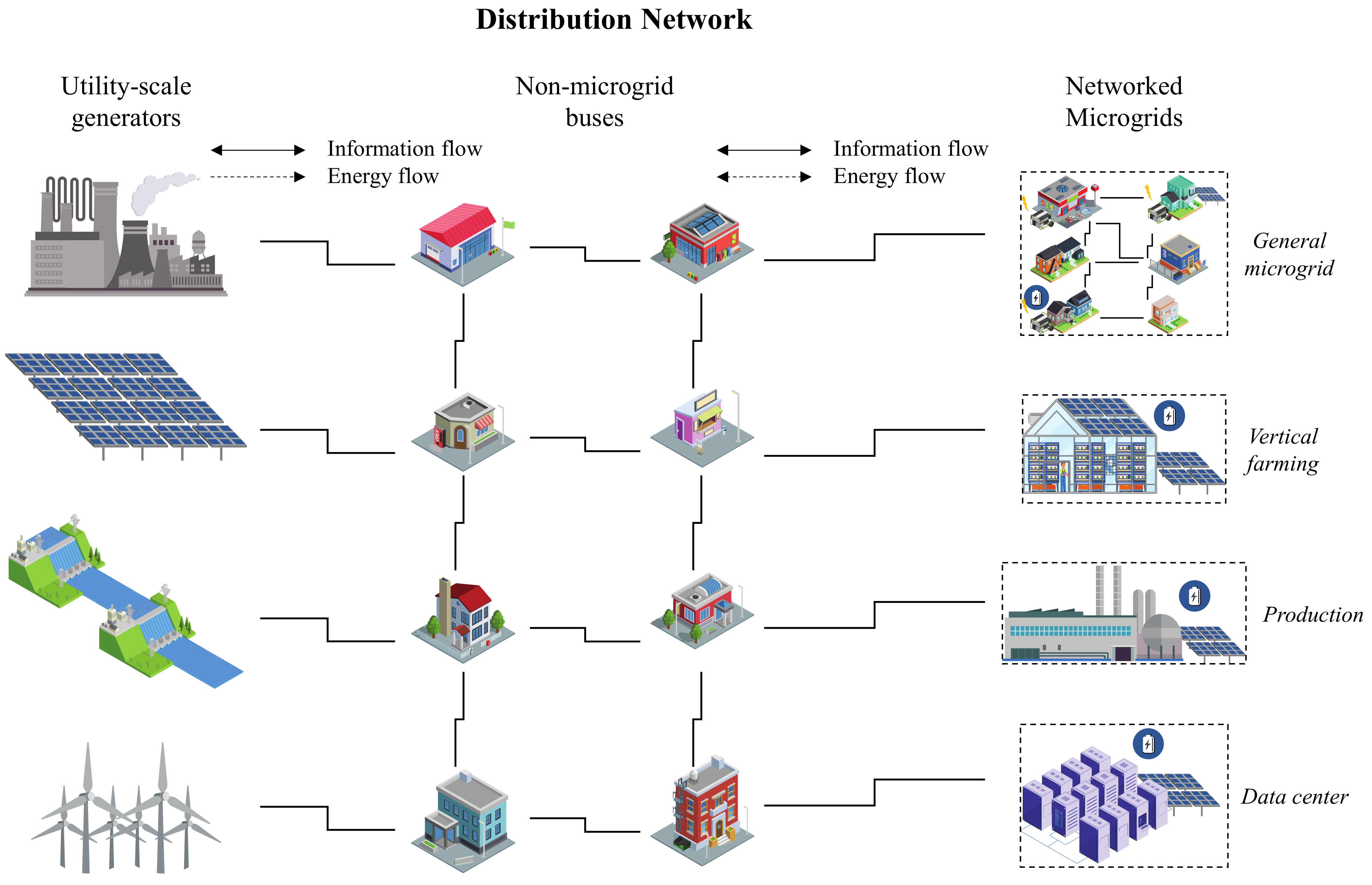Each microgrid $m\in \mathcal{M}$ can satisfy its demand via a combination of onsite energy generation and storage technologies, as well as energy purchased from the DN. The microgrid can decide to accept a reduction in their energy consumption levels when the DNO requests them. Furthermore, the microgrid has the capability of selling the surplus of onsite produced energy to the DN. Each microgrid has different characteristics depending on the system it represents, and its goal is to find its optimal operational and energy decisions. The microgrids under study include residential facilities, manufacturing facilities, data centers, and agricultural facilities. The system is shown in Figure 1, in which the large-scale generators are on the left-hand side of the figure, the non-microgrids buses are in the middle, and the microgrid buses are on the right-hand side.

The mathematical formulation is presented below.

Table 1. Sets and indices.

Symbol	Description
$\mathcal{T}$	Set of time frames in the planning horizon, indexed by $t\in \{1,2,\dots ,T\}$, $T=\left|\mathcal{T}\right|$
$\mathcal{I}$	Set of buses, indexed by i
$\mathcal{M}\subseteq \mathcal{I}$	Set of microgrid buses, indexed by m (connected to bus $i_m\in \mathcal{I}$)
$\mathcal{E}$	Set of transmission lines, indexed by e (denoted by $e=(i_e,j_e)$, with tail bus $i_e$ and head bus $j_e$)
$\mathcal{G}$	Set of conventional energy generators, indexed by g (connected to bus $i_g\in \mathcal{I}$)
$\mathcal{R}$	Set of renewable energy generators, indexed by r (connected to bus $i_r\in \mathcal{I}$)
$\mathcal{K}$	Set of consumption levels for dynamic tariff policy, indexed by k

,

Table 2. Model parameters.

Symbol	Description
${\underline{P}}_g^G/{\overline{P}}_g^G$	Lower/upper limits of power output for generation unit g
$T_g^{d0/u0}$	Minimum number of periods generation unit g must be initially offline/online
$T_g^{d/u}$	Minimum number of periods generation unit g must remain offline/online once it is shut down/started up
${\tilde{R}}_g^{d/u}$	Maximum shutdown/startup ramping rate for generation unit $g\in \mathcal{G}$ when is shut down/started up
$R_g^{d/u}$	Maximum ramp-down/up rate for generation unit g between adjacent periods
$C_g^{Td/Tu}$	Fixed shutdown/startup cost for generation unit g
$C_g^{Rd/Ru}$	Ramp-down/up unitary cost for generation unit g
$C_g^P$	Generation cost function for generation unit g
$F_e$	Capacity of transmission line e
$B_e$	Susceptance of transmission line e
${\overline{P}}_{m,t}^{F/N}$	Limit under Firm (F)/Non-firm (N) contract for power purchased from microgrid m, at period t
$C_{m,t}^{F/N}$	Cost of power purchased from microgrid m, under Firm (F)/Non-firm (N) contract, at period t
$D_{i,k,t}$	Energy demand at bus i, at consumption level k, at period t
$C_{m,k,t}^{In}$	Load reduction incentive per unit offered to microgrid m, at consumption level k, at period t
$C_r^R$	Production cost of renewable type r
$C_{i,k,t}^{DT}$	Energy price for bus i at consumption level k, at period t
$C_{i,k,t}^S$	Cost of load shedding per unit on bus i, at consumption level k, at time t
${\overline{P}}_{r,t}^R$	Availability of renewable power of RES type r at period t
${\overline{P}}_{i,k,t}^{DT}$	Amount of conventional energy available at bus i, at consumption level k, at period t
${\overline{Q}}_{m,k,t}$	Limit for load reduction requests for microgrid m, at consumption level k, at period t

and

Table 3. Decision variables.

Symbol	Description
$x_{g,t}\in \{0,1\}$	Binary variable indicating if generation unit g is committed ($x_{g,t}=1$) or not ($x_{g,t}=0$) at period t
$y_{g,t}^{u/d}\in \{0,1\}$	Binary variable indicating if generation unit g is started up/shut down ($y_{g,t}^{u/d}=1$) or not ($y_{g,t}^{u/d}=0$) at period t
$p_{g,t}^{G+/G-}$	Electricity generation/curtailment of conventional generator g at period t
$p_{g,t}^G$	Power supplied from generator g to the DN at period t
$p_{g,t}^{u/d}$	Ramp up/down of conventional generator g at period t
$p_{r,t}^R$	Electricity generation of renewable generator r at period t
$f_{e,t}$	Electricity flow on line e, at period t
$z_{e,t}\in \{0,1\}$	Binary variable indicating if line e is switched on ($z_{e,t}=1$) or off ($z_{e,t}=0$), at period t
${\theta }_{i_e,t}$	Voltage angle of bus i on line e, at period t
$p_{m,t}^{F/N}$	Electricity purchased from microgrid m, under Firm (F)/Non-firm (N) contract, at period t
$p_{i,k,t}^{(-)}$	Electricity sold to bus i, at consumption level k at period t
$q_{m,k,t}$	Amount of load reduction requested to microgrid m, at consumption level k, at period t
$s_{i,k,t}$	Amount of load shed from bus i, at consumption level k, at period t

summarize the nomenclature utilized in the formulation. In particular, Table 1 lists the sets and indices for the time horizon, buses, microgrids, transmission lines, conventional and renewable generators, and dynamic electricity tariffs. Table 2 presents the costs associated with unit commitment, electricity generation and ramping, electricity purchased, and load shedding; the sales price of electricity; electricity generation and ramping capacities, as well as electricity trades limits; capacity and susceptance of transmission lines; and electricity demand of the buses. Table 3 lists the decision variables, including unit commitment, power generation, and ramping, energy flow in the transmission lines, power sold to and bought from microgrids, load reductions, and load shedding.

3.1. The Distribution Network

The DN needs to find the day-ahead schedule of the conventional generation units, the power used from the renewable generators, the optimal power flow, the energy transactions with the microgrids, the application of DR policies, and the energy balance that minimize the cost.

3.1.1. Unit Commitment

Since utility-scale conventional generators require larger periods to change their status, the problem of finding their optimal scheduling problem has been well studied. The unit commitment problem refers to the decisions of starting up and shutting down generators. A modified version of the unit commitment problem presented in [44] is shown in Equations (1)–(8).

$$\begin{array}{cc}\hfill \sum _{t=1}^{T_g^{u0}}(1-x_{g,t})=0,& \forall g\in \mathcal{G}\hfill \end{array}$$

(1)

$$\begin{array}{cc}\hfill \sum _{t=1}^{T_g^{d0}}{x}_{g,t}=0,& \forall g\in \mathcal{G}\hfill \end{array}$$

(2)

$$\begin{array}{cc}\hfill \sum _{t^{\prime }=t}^{t+T_g^u-1}{x}_{g,t^{\prime }}\ge T_g^u·y_{g,t}^u,& \forall g\in \mathcal{G},t\in \{T_g^{u0}+1,\dots ,T-T_g^u+1\}\hfill \end{array}$$

(3)

$$\begin{array}{cc}\hfill \sum _{t^{\prime }=t}^{t+T_g^d-1}(1-x_{g,t^{\prime }})\ge T_g^d·y_{g,t}^d,& \forall g\in \mathcal{G},t\in \{T_g^{d0}+1,\dots ,T-T_g^d+1\}\hfill \end{array}$$

(4)

$$\begin{array}{cc}\hfill \sum _{t^{\prime }=t}^T(x_{g,t^{\prime }}-y_{g,t}^u)\ge 0,& \forall g\in \mathcal{G},t\in \{T-T_g^u+2,\dots ,T\}\hfill \end{array}$$

(5)

$$\begin{array}{cc}\hfill \sum _{t^{\prime }=t}^T\left((1-x_{g,t^{\prime }})-y_{g,t}^d\right)\ge 0,& \forall g\in \mathcal{G},t\in \{T-T_g^d+2,\dots ,T\}\hfill \end{array}$$

(6)

$$\begin{array}{cc}\hfill y_{g,t}^u-y_{g,t}^d=x_{g,t}-x_{g,t-1},& \forall g\in \mathcal{G},t\in \mathcal{T}\hfill \end{array}$$

(7)

$$\begin{array}{cc}\hfill x_{g,t},y_{g,t}^u,y_{g,t}^d\in \{0,1\},& \forall g\in \mathcal{G},t\in \mathcal{T}\hfill \end{array}$$

(8)

Constraints (1) and (2) represent the initial online/offline requirements for generation unit g, which consists of $T_g^{u0}$ and $T_g^{d0}$ periods, respectively. The minimum number of periods that the generator unit g must remain online/offline after the minimum initial online/offline periods is represented by (3) and (4) ($T_g^u$ and $T_g^d$ periods, respectively). These constraints are modified to account for the minimum number of periods that the generator unit g must remain online/offline at the end of the time horizon, as presented on (5) and (6). The relationship between starting up/shutting down generator unit g, represented by binary variables $y_{g,t}^u$ and $y_{g,t}^d$, respectively, and its commitment status, modeled as the binary variable $x_{g,t}$, is modeled in (7). The binary requirements for the decision of the online/offline status as well as the starting up/shutting down the generator unit g are modeled in (8).

3.1.2. Conventional Power Generation

The amount of power that the utility-scale generators produce, modeled as $p_{g,t}^{G+}$, is bounded by the lower and upper limits (${\underline{P}}_g^G$ and ${\overline{P}}_g^G$, respectively) determined by their technical capacities. Additionally, a generator can contribute only if it is turned on during a certain period. The power generation is shown in Equations (9)–(14).

$$\begin{array}{cc}\hfill {\underline{P}}_g^G{x}_{g,t}\le p_{g,t}^{G+}\le {\overline{P}}_g^G{x}_{g,t},& \forall g\in \mathcal{G},t\in \mathcal{T}\hfill \end{array}$$

(9)

$$\begin{array}{cc}\hfill p_{g,t}^{G+}=p_{g,t-1}^{G+}+p_{g,t}^u-p_{g,t}^d,& \forall g\in \mathcal{G},t\in \mathcal{T}\hfill \end{array}$$

(10)

$$\begin{array}{cc}\hfill 0\le p_{g,t}^u\le R_g^u·x_{g,t-1}+{\tilde{R}}_g^u·y_{g,t}^u,& \forall g\in \mathcal{G},t\in \mathcal{T}\hfill \end{array}$$

(11)

$$\begin{array}{cc}\hfill 0\le p_{g,t}^d\le R_g^d·x_{g,t}+{\tilde{R}}_g^d·y_{g,t}^d,& \forall g\in \mathcal{G},t\in \mathcal{T}\hfill \end{array}$$

(12)

$$\begin{array}{cc}\hfill 0\le p_{g,t}^{G-}\le p_{g,t}^{G+},& \forall g\in \mathcal{G},t\in \mathcal{T}\hfill \end{array}$$

(13)

$$\begin{array}{cc}\hfill p_{g,t}^G=p_{g,t}^{G+}-p_{g,t}^{G-},& \forall g\in \mathcal{G},t\in \mathcal{T}\hfill \end{array}$$

(14)

A generator g can produce power only if it is online, as modeled in (9). Generator unit g can change its power supply depending on its ramping rates, which determine how fast the electricity generation can be increased ($p_{g,t}^u$) or decreased ($p_{g,t}^d$) per unit time, or when the generator is turned on/off; this is modeled in (10). The generator’s ramping rate limits are presented in equations (11) and (12), where $R_g^u$ and $R_g^d$ represent the increase/decrease ramping limits when the generator is online, whereas ${\tilde{R}}_g^u$ and ${\tilde{R}}_g^d$ represent the increase/decrease ramping rates when the generator has started up or is shut down, respectively. In the case that the power generation of unit g is more than the required amount, it is possible to curtail some of that power to achieve power balance; the power curtailed, modeled as $p_{g,t}^{G-}$, cannot be larger than the power generated, as modeled in (13). The amount of power supplied to the DN is modeled as $p_{g,t}^G$ in (14).

3.1.3. Renewable Power Generation

For utility-scale renewable generators, the renewable power, modeled as $p_{r,t}^R$, is considered to depend only on the renewable power availability, ${\overline{P}}_{r,t}^R$. The amount of renewable power that can be generated is presented in Equation (15).

$$0\le p_{r,t}^R\le {\overline{P}}_{r,t}^R,\forall r\in \mathcal{R},t\in \mathcal{T}$$

(15)

For this paper, the available renewable power is treated as uncertain. The integration of this uncertainty in the proposed model is discussed in Section 3.3.

3.1.4. Transmission Lines

A network topology is utilized to model the DN. Transmission lines can be considered as the edges of the network, while the buses are analogous to the nodes. The power flow that is generated on a bus i can satisfy the demand on a bus j if there is a path that connects buses i and j through transmission lines. The initial node of transmission line e is modeled as $i_e$ and its end node is modeled as $j_e$. The dynamics of transmission lines are modeled as the DC approximation for the optimal power flow problem, as presented in Equations (16)–(18).

$$\begin{array}{cc}\hfill -F_e·z_{e,t}\le f_{e,t}\le F_e·z_{e,t},& \forall e\in \mathcal{E},t\in \mathcal{T}\hfill \end{array}$$

(16)

$$\begin{array}{cc}\hfill f_{e,t}=B_e·({\theta }_{i_e,t}-{\theta }_{j_e,t})·z_{e,t},& \forall e\in \mathcal{E},t\in \mathcal{T}\hfill \end{array}$$

(17)

$$\begin{array}{cc}\hfill z_{e,t}\in \{0,1\},& \forall e\in \mathcal{E},t\in \mathcal{T}\hfill \end{array}$$

(18)

The flow in transmission line e, modeled as $f_{e,t}$, is bounded by its physical capacity, $F_e$, and the line switching status, $z_{e,t}$, as modeled in (16). Kirchhoff’s law for the DC optimal power flow problem, which considers that the power flow in a transmission line within the microgrid is proportional to the difference of the voltage phase angles at the terminal buses of the line (${\theta }_{i_e,t}$ and ${\theta }_{j_e,t}$) and the line’s susceptance ($B_e$), taking into account the decision of connecting/disconnecting the transmission line as modeled in (17). The connected/disconnected binary status of the transmission lines is modeled in (18). Note that (17) involves a nonlinear term. Then, it can be reformulated as presented in (19).

$$B_e·({\theta }_{i_e,t}-{\theta }_{j_e,t})-(1-z_{e,t})·F_e\le f_{e,t}\le B_e·({\theta }_{i_e,t}-{\theta }_{j_e,t})+(1-z_{e,t})·F_e,\forall e\in \mathcal{E},t\in \mathcal{T}$$

(19)

3.1.5. Electricity Bought from Microgrids

The DNO has to supply electricity to every bus in the network. In the case of microgrids, it is assumed that they have electricity production capacity through distributed generation. It can be the case that the microgrid produces more electricity than the requirements for its operation. In this case, the DNO can leverage this surplus of electricity to satisfy other buses in the network by purchasing it from the microgrids. This type of transaction can be carried out at different rates. The electricity traded under a contract limit is called firm, modeled as $p_{m,t}^F$, and any amount of electricity traded beyond the contract limit is considered non-firm, modeled as $p_{m,t}^N$. The trade prices for both firm and non-firm purchases are different. The constraints for the connection and trades between the DNO and the microgrids are modeled in the Equations (20)–(22).

$$\begin{array}{cc}\hfill \sum _{k\in \mathcal{K}}{p}_{i_m,k,t}^{(-)}-(p_{m,t}^N+p_{m,t}^F)=\sum _{e\in \mathcal{E}:j_e=i_m}{f}_{e,t},& \forall m\in \mathcal{M},t\in \mathcal{T}\hfill \end{array}$$

(20)

$$\begin{array}{cc}\hfill 0\le p_{m,t}^F\le {\overline{P}}_{m,t}^F,& \forall m\in \mathcal{M},t\in \mathcal{T}\hfill \end{array}$$

(21)

$$\begin{array}{cc}\hfill 0\le p_{m,t}^N\le {\overline{P}}_{m,t}^N,& \forall m\in \mathcal{M},t\in \mathcal{T}\hfill \end{array}$$

(22)

The total power flow in the transmission lines between the DNO and microgrid m is modeled in (20), where the left-hand side represents the net trade calculated by subtracting the electricity supplied from the microgrid to the DN from the energy sold to the microgrid node, modeled as $p_{i_m,k,t}^{(-)}$. The limits of the power that can be traded under firm and non-firm contracts, ${\overline{P}}_{m,t}^F$ and ${\overline{P}}_{m,t}^N$, are modeled in (21) and (22), respectively.

3.1.6. Demand Response

In this paper, two DR policies are considered: DT and load-reduction incentives. Particularly, the DT policy is modeled for the power sold to the buses. Therefore, the demand at each bus i is divided based on the |$\mathcal{K}$| consumption levels of the DT policy and represented by $D_{i,k,t}$. Moreover, if bus i represents a microgrid, the DNO may request a load reduction of $q_{m,k,t}$ units of electricity at a particular period t. If the DNO is still unable to satisfy that demand, it is possible to incur load shedding of $s_{i,k,t}$ units of electricity. The amount of electricity sold to bus i after the above-mentioned considerations is modeled in Equations (23)–(25).

$$\begin{array}{cc}\hfill p_{i,k,t}^{(-)}=D_{i,k,t}-s_{i,k,t}-q_{i_m,k,t},& \forall i\in \mathcal{I},k\in \mathcal{K},t\in \mathcal{T}\hfill \end{array}$$

(23)

$$\begin{array}{cc}\hfill 0\le q_{m,k,t}\le {\overline{Q}}_{m,k,t},& \forall m\in \mathcal{M},k\in \mathcal{K},t\in \mathcal{T}\hfill \end{array}$$

(24)

$$\begin{array}{cc}\hfill 0\le s_{i,k,t}\le D_{i,k,t},& \forall i\in \mathcal{I},k\in \mathcal{K},t\in \mathcal{T}\hfill \end{array}$$

(25)

The electricity sold to bus i equals its demand minus the load that is shed, and, in the case of microgrid nodes, minus the amount that is requested to reduce, as modeled in (23). The maximum amount that can be requested to be reduced from microgrids at each DT level is modeled as ${\overline{Q}}_{m,k,t}$ in (24). The load that can be shed from a certain bus cannot be greater than the demand of this bus, as modeled in (25).

Note that the design of the set of equations to model the power sold to each bus allows other pricing policies, such as real-time pricing and critical peak pricing, by modifying the price parameters on each time frame t, which are discussed in Section 3.1.8.

3.1.7. Power Balance

The power supply and demand balance should be satisfied at each of the nodes of the DN. Equation (26) represents the power balance at bus i for each time frame t. The power supply (in the left-hand side of the equation) is the sum of the power generated by conventional and renewable generators placed at bus i and the incoming power flow. The power demand (on the right-hand side of the equation) is the power sold to bus i and the sum of the outgoing power flow.

$$\sum _{g:i_g=i}{p}_{g,t}^G+\sum _{r:i_r=i}{p}_{r,t}^R+\sum _{e:j_e=i}{f}_e=\sum _{k\in \mathcal{K}}{p}_{i,k,t}^{(-)}+\sum _{e:i_e=i}{f}_e,\forall i\in \mathcal{I},t\in \mathcal{T}$$

(26)

3.1.8. Cost Management

The cost function consists of the production cost for conventional and renewable generators, the ramping and commitment processes of the conventional generators and load shedding, the revenues obtained for selling electricity under DT policy, as well as the incentives paid for load reduction requests accepted by the microgrids. In general, the unit commitment and power generation costs are nonlinear and nonconvex. A linear approximation of the cost function consisting of a piecewise-linear reformulation based on the AC optimal power problem flow is presented in this paper. The unit commitment cost associated with starting and shutting down the generators, $c_{\mathrm{UC}}$, is shown in Equation (27).

$$c_{\mathrm{UC}}=\sum _{t\in \mathcal{T}}\sum _{g\in \mathcal{G}}\left(C_g^{Tu}·y_{g,t}^u+C_g^{Td}·y_{g,t}^d\right),$$

(27)

where $C_g^{Tu}$ and $C_g^{Td}$ represent the cost for starting up and shutting down the conventional generators, respectively.

The power generation and ramping cost for both conventional and renewable generators, $c_{\mathrm{PG}}$, are shown in Equation (28).

$$c_{\mathrm{PG}}=\sum _{t\in \mathcal{T}}\left(\sum _{g\in \mathcal{G}}\left(C_g^P·p_{g,t}^{G+}+C_g^{Ru}·p_{g,t}^u+C_g^{Rd}·p_{g,t}^d\right)+\sum _{r\in \mathcal{R}}{C}_r^R·p_{r,t}^R\right),$$

(28)

where $C_g^P$, $C_g^{Ru}$, $C_g^{Rd}$ and $C_r^R$ indicate the generation cost, ramping up, and raping down of conventional generators, as well as the generation cost of renewable generators, respectively.

The cost of the electricity purchased from the microgrids and the incentives paid for accepting load reductions, $c_{\mu \mathrm{G}}$, are shown in Equation (29).

$$c_{\mu \mathrm{G}}=\sum _{t\in \mathcal{T}}\sum _{m\in \mathcal{M}}\left(C_{m,t}^F·p_{m,t}^F+C_{m,t}^N·p_{m,t}^N+\sum _{k\in \mathcal{K}}{C}_{m,k,t}^{In}·q_{m,k,t}\right),$$

(29)

where $C_{m,t}^F$, $C_{m,t}^N$ and $C_{m,k,t}^{In}$ model the cost of energy purchased from the microgrids under firm and non-firm contracts, as well as the load reduction incentives per electricity unit, respectively.

The cost of load shedding from different buses of the DN, $c_{\mathrm{Sh}}$, is reflected in Equation (30). Note that, depending on the criticality level of a given bus, the load shedding penalty $C_{i,k,t}^S$ can be adjusted, e.g., this parameter can be relatively low for a residential bus, and very high for a hospital.

$$c_{\mathrm{Sh}}=\sum _{t\in \mathcal{T}}\sum _{k\in \mathcal{K}}\sum _{i\in \mathcal{I}}\left(C_{i,k,t}^S·s_{i,k,t}\right)$$

(30)

Finally, the revenue obtained from selling energy at different DT levels, $c_{\mathrm{DT}}$, is shown in (31). Note that the definition of the DT parameters $C_{i,k,t}^{DT}$ allows the model to be flexible to utilize different tariffs schemes, such as TLOU (used in this paper), real-time pricing (by using different values on each time frame), and critical peak pricing (by setting very high values in particular time frames).

$$c_{\mathrm{DT}}=\sum _{t\in \mathcal{T}}\sum _{k\in \mathcal{K}}\sum _{i\in \mathcal{I}}\left(C_{i,k,t}^{DT}·p_{i,k,t}^{(-)}\right)$$

(31)

3.1.9. Optimization Model

The optimization model for the operation of the DNO consists of minimizing the total cost, subject to the operational constraints. In order to facilitate the discussion of the solution methodology, a compact form of the problem is presented in (32). Let vector $\mathbf{x}$ represent the unit commitment (binary) decision variables, $x_{g,t},y_{g,t}^u,y_{g,t}^d$; vector $\mathbf{y}$ denote the power generation and power flow (continuous) decision variables, $p_{g,t}^{G+/G-/G}$, $p_{g,t}^{u/d}$, $p_{r,t}^R$, $f_{e,t}$, ${\theta }_{i_e,t}$, $p_{m,t}^{F/N}$, $p_{i,k,t}^{(-)}$, $q_{m,t}$, and $s_{i,t}$; and vector $\mathbf{z}$ represents the line switching (binary) decision variables, $z_{e,t}$.

$$\begin{array}{c}\hfill \begin{array}{cc}\hfill \underset{\mathbf{x},\mathbf{y},\mathbf{z}}{min}& c_{\mathrm{UC}}+c_{\mathrm{PG}}+c_{\mu \mathrm{G}}+c_{\mathrm{Sh}}-c_{\mathrm{DT}}\hfill \\ \mathrm{s}.\mathrm{t}.\hfill & \mathrm{Constraints}\left(1\right)–\left(16\right),\left(18\right)–\left(26\right)\hfill \end{array}\end{array}$$

(32)

3.2. The Microgtrids

In this paper, it is assumed that each microgrid is capable of making its own operational and energy decisions. Optimal control techniques for microgrids are discussed in more detail by Minchala-Avila et al. [45]. It is out of the scope of this paper to get into the details for each type of microgrid but is assumed, without loss of generality, that their management team utilizes mathematical optimization to find their optimal operation. A general cost minimization model for the optimal operation and energy decisions of microgrids that considers DSM policies can be modeled as shown in (33)–(36).

$$\begin{array}{cc}\hfill \underset{\mathbf{o},\mathbf{p}|{\delta }_{DSM}}{min}& f(\mathbf{o},\mathbf{p})\hfill \end{array}$$

(33)

$$\begin{array}{cc}\hfill \mathrm{s}.\mathrm{t}.& g(\mathbf{o},\mathbf{p})\le 0\hfill \end{array}$$

(34)

$$\begin{array}{cc}\hfill & \mathbf{o}\in \mathcal{O}\hfill \end{array}$$

(35)

$$\begin{array}{cc}\hfill & \mathbf{p}\in \mathcal{P},\hfill \end{array}$$

(36)

where $\mathbf{o}$ and $\mathbf{p}$ represent the operational and energy decisions, respectively, ${\delta }_{DSM}$ represents the DSM policies used by the DNO, and constraints (34)–(36) represent the operational and energy constraints. In this paper, ${\delta }_{DSM}$ is composed of the incentives offered for load reduction requests, $C_{m,k,t}^{In}$; the load reduction requested by the DNO, ${\overline{q}}_{m,k,t}$; the DT levels, ${\overline{P}}_{i_m,k,t}^{DT}$; the DT prices, ${\overline{C}}_{i_m,k,t}^{DT}$; the price of the energy bought at firm and non-firm contracts, $C_{m,t}^F$ and $C_{m,t}^N$, respectively; and the maximum amount of the firm and non-firm contracts, ${\overline{P}}_{m,t}^F$ and ${\overline{P}}_{m,t}^N$, respectively.

To achieve the optimal coordination of operational and energetic goals, an EMS is assumed to be installed within each microgrid to jointly optimize the use of energy and its operations. Figure 2 presents the scheme for a microgrid with a central EMS that utilizes information from the operational requirements, as well as the available onsite energy technologies and the DN, finding the optimal operations.

It is assumed that each microgrid can generate and store its own electricity, and utilize the electricity from the DN to optimize its processes. The EMS considers information, such as costs and incentives offered by the DN, including the DSM policies, to optimally decide how much energy to purchase or sell to the DN. It is assumed that the microgrid’s EMS will produce and communicate the following information to the DNO:

• The amount of energy consumed from the grid at each DT level, $D_{i_m,k,t}$.
• The amount of energy sold to the grid under firm and non-firm contracts, ${\widehat{p}}_{m,t}^{F/N}$.
• The amount of electricity consumption willing to reduce, ${\widehat{q}}_{m,k,t}$.

The information obtained from each microgrid can be used by the DNO to find its optimal operation.

The microgrids considered in this paper are classified into three categories, based on the definition of energy-consuming sectors defined by the U.S. EIA [46]:

(1)

Residential microgrids: The residential sector consists of living quarters for private households. Residential microgrids include the operation of appliances such as space heating, water heating, air conditioning, lighting, refrigeration, cooking, and running a variety of other appliances. Some of the residential appliances allow certain flexibility in the time frames they need to be operated. As an example, a washing machine can be scheduled to operate during specific periods that optimize energy usage.

(2)

Industrial microgrids: The industrial sector consists of facilities and equipment used for producing, processing, or assembling goods. This sector encompasses agriculture, forestry, fishing, hunting, mining, oil and gas extraction, and construction. Industrial microgrids present flexibility in their operation as long as the demand of goods is satisfied during the planning horizon. A change in their operation results in a change in their energy consumption patterns.

(3)

Commercial microgrids: The commercial sector consists of service-providing facilities and equipment of businesses, governments, and other private and public organizations. Common uses of energy associated with this sector include space heating, water heating, air conditioning, lighting, refrigeration, cooking, and running a wide variety of other equipment. Commercial microgrids present a certain flexibility in their operation, as long as a certain quality of service level is satisfied. Similarly to the industrial microgrids, a change in their operation results in a change in their energy consumption patterns.

3.3. Solution Methodology

In this section, the solution approach for the DN alone is presented in Section 3.3.1, and the framework for the collaboration between the DN and the microgrids is presented in Section 3.3.2.

3.3.1. Optimal Operation of the Distribution Network

In mathematical optimization, uncertainty can be addressed by finding the optimal operation of the system under the most adverse scenario with robust optimization. It is suitable for assessments in the long term, e.g., to compare the performance of the system after applying certain DSM policies. It is also suitable for short-term decisions since it can be assumed that, if the system can perform successfully in the worst-case scenario, then it can perform successfully in any other scenario as well.

The uncertainty of the presented model comes from the renewable power availability, ${\overline{P}}_{r,t}^R$, given that its intermittency depends on weather conditions. Nevertheless, it is assumed that the expected value, $\mathbb{E}\left[{\overline{P}}_{r,t}^R\right]$, and the variance, $\mathrm{Var}\left[{\overline{P}}_{r,t}^R\right]$, of the renewable power output at each period can be obtained. Then, an uncertainty set, $\mathcal{U}$, can be constructed utilizing the mean and the standard deviation, without a loss of generality. For the purpose of this paper, the uncertainty set is constructed by a lower bound and an upper bound, defined as follows:

$$\mathcal{U}=\left\{\begin{array}{c}{\overline{P}}_{r,t}^R\in [\mathbb{E}\left[{\overline{P}}_{r,t}^R\right]-{\underline{\mathrm{Y}}}_{r,t},\mathbb{E}\left[{\overline{P}}_{r,t}^R\right]+{\overline{\mathrm{Y}}}_{r,t}],\forall r\in \mathcal{R},t\in \mathcal{T}\end{array}\right\}$$

(37)

where ${\underline{\mathrm{Y}}}_{r,t}$ and ${\overline{\mathrm{Y}}}_{r,t}$ denote the deviations that define the lower and upper bounds for a renewable source r at period t, and are a function of the variance. For this paper, ${\underline{\mathrm{Y}}}_{r,t}={\overline{\mathrm{Y}}}_{r,t}={\mathrm{Var}\left[{\overline{P}}_{r,t}^R\right]}^{1/2}$. To determine the specific solar availability, auxiliary variables ${\underline{\upsilon }}_{r,t}$ and ${\overline{\upsilon }}_{r,t}$ are used to measure the deviation from the mean value, and a budget of uncertainty, U, limits the total deviation. The uncertainty set (37) can be formulated as follows:

$$\begin{array}{cc}\hfill {\overline{P}}_{r,t}^R=\mathbb{E}\left[{\overline{P}}_{r,t}^R\right]-{\underline{\upsilon }}_{r,t}·{\underline{\mathrm{Y}}}_{r,t}+{\overline{\upsilon }}_{r,t}·{\overline{\mathrm{Y}}}_{r,t},& \forall r\in \mathcal{R},t\in \mathcal{T}\hfill \\ \hfill 0\le {\underline{\upsilon }}_{r,t},{\overline{\upsilon }}_{r,t}\le 1,& \forall r\in \mathcal{R},t\in \mathcal{T}\hfill \\ \hfill \sum _{t\in \mathcal{T}}\sum _{r\in \mathcal{R}}({\underline{\upsilon }}_{r,t}+{\overline{\upsilon }}_{r,t})\le U\end{array}$$

By design, the budget of uncertainty allows the DNO to control the level of conservativeness utilized in the planning process. If the DNO sets $U=0$, the renewable power output parameters are fixed to the mean value at each period; on the other hand, if $U=T·\left|\mathcal{R}\right|$, it allows each renewable source to vary during all the time frames during the planning horizon.

The problem of finding the optimal operation of the DN with networked microgrids can be analyzed in two stages: First, the DNO finds the optimal unit commitment decisions for day-ahead planning. After this, the conventional and renewable generators produce the energy under the operational constraints and distribute it via the power grid. Note that the unit commitment occurs before the availability of the intermittent renewable sources is revealed in the first stage, and the power flow and line switching decisions occur in the second stage, once the renewable availability is unfolded. The model stated in (32) can be rewritten to follow the robust optimization approach as follows:

$$\begin{array}{c}\hfill \begin{array}{c}\hfill \underset{\mathbf{x}}{min}{c}_{\mathrm{UC}}+\underset{\mathbf{r}\in \mathcal{U}}{max}\underset{\mathbf{y},\mathbf{z}|\widehat{\mathbf{x}}}{min}{c}_{\mathrm{PG}}+c_{\mu \mathrm{G}}+c_{\mathrm{Sh}}-c_{\mathrm{DT}}\\ \hfill \mathrm{s}.\mathrm{t}.\mathrm{Constraints}\left(1\right)–\left(16\right),\left(18\right)–\left(26\right)\end{array}\end{array}$$

(38)

where vector $\mathbf{r}$ denotes the uncertain parameters of renewable availability, ${\overline{P}}_{r,t}^R$. The optimization model finds the worst-case renewable availability by utilizing the operator ${max}_{\mathbf{r}\in \mathcal{U}}$. This can be understood as follows: While the DNO tries to minimize the operational cost by controlling the unit commitment (${min}_{\mathbf{x}}$) and power flow (${min}_{\mathbf{y},\mathbf{z}}$), another “agent” (i.e., the uncontrollable weather conditions) tries to maximize the cost by adjusting the renewable power availability (${max}_{\mathbf{r}\in \mathcal{U}}$). The resulting problem is a two-stage MILP problem, in which the first stage has only binary variables, while the second stage has both continuous and binary variables. This structure can be solved utilizing a nested column- and-constraint-generation approach, as demonstrated in [31].

3.3.2. Coordination between DNO and the Microgrids

The DNO and the microgrids try to optimize their operations and there may exist conflicting objectives, considering that the DN business consists of selling electricity to the latter, while the microgrids seek to minimize their operational costs, including the energy purchase. It is assumed that the DNO does not have direct control of the operation of the microgrids nor complete information of the microgrids’ internal systems. Nevertheless, the DNO leverages the DSM policies to influence the behavior of the microgrids, but the microgrids have the last decision on their operation. In this paper, the collaboration process is considered as follows: First, each of the microgrids presents an estimation of their electricity demand to the DNO, without considering any reduction request or power traded to the DN. Second, the DNO uses the consumption estimated by the microgrids to assess its operation and requests load reduction to each of the microgrids, with their respective incentives. Third, the microgrids consider the load reduction requests and the possibility of trading power to the DNO under firm and non-firm contracts, resulting in a new estimation for demand. Finally, the DNO uses the information of the accepted requests and power available from the microgrids to find its optimal operation. This approach can be summarized in the following algorithm:

• Let the following elements on ${\delta }_{DSM}$ be equal to zero: $C_{m,k,t}^{In}$, ${\overline{q}}_{m,k,t}$, $C_{m,t}^F$, $C_{m,t}^N$, ${\overline{P}}_{m,t}^F$ and ${\overline{P}}_{m,t}^N$, and solve each of the microgrids optimization models to obtain $D_{i_m,k,t}$.
• Let ${\overline{Q}}_{m,k,t}=D_{i_m,k,t}$, and ${\overline{P}}_{m,t}^F={\overline{P}}_{m,t}^N=0$ and solve the DNO optimization model in (38) to obtain $q_{m,k,t}^{\ast }$.
• Let all elements of ${\delta }_{DSM}$ take their original values, and ${\overline{q}}_{m,k,t}=q_{m,k,t}^{\ast }$, and solve each of the microgrids optimization models to obtain $D_{i_m,k,t}$, ${\widehat{p}}_{m,t}^{F/N}$, and ${\widehat{q}}_{m,k,t}$.
• Let ${\overline{Q}}_{m,k,t}=0$, ${\overline{P}}_{m,t}^F={\widehat{p}}_{m,t}^F$ and ${\overline{P}}_{m,t}^N={\widehat{p}}_{m,t}^N$ and solve the DNO optimization model shown in (38) with the updated values obtained from the microgrids, adding the following term to its optimal cost ${\sum }_{t\in \mathcal{T}}{\sum }_{k\in \mathcal{K}}{\sum }_{m\in \mathcal{M}}\left(C_{m,k,t}^{In}·{\widehat{q}}_{m,k,t}\right)$, which represents the cost paid to the microgrids for accepting the load reduction requests.

4. Results

The algorithms and formulations presented in this paper were implemented using the C++ API of CPLEX 20.10 via ILOG Concert Technology. The hardware utilized consists of a DELL machine with Intel(R) Core(TM) i7-10700 CPU 2.90 GHz (eight-core) processor and 32 GB RAM, and it runs on Microsoft Windows 10. The computational time is reported as CPU seconds. For testing the framework discussed above, a benchmark case was carried out and compared with different configurations to demonstrate the flexibility of the proposed approach. The following experiments were carried out: (1) The benchmark case in Section 4.2 was studied under the configuration presented in Section 4.1; (2) In the case presented in Section 4.3, the settings of the conventional generators set, $\mathcal{G}$, were modified to improve the results obtained in the benchmark case; (3) In the case presented in Section 4.4, the size of the renewable energy generators in both the DN and the microgrids was doubled. The second and third experiments are examples of long-term planning decisions.

4.1. Case Settings

A modified version of the IEEE 30-Bus System [47] was utilized as the DN. The operation of the DN was evaluated for a daily horizon divided into $\left|\mathcal{T}\right|=24$ periods, each corresponding to one hour. Within the DN, $\left|\mathcal{M}\right|=5$ microgrids are included in buses 5, 11, 18, 26, and 29. Each of the microgrids have onsite technologies of energy storage and PV farms, as well as an EMS that finds its optimal operation considering both the operational and energy constraints, as described in Section 3.2. The microgrid in bus 5 is a manufacturing facility with multi-process production scheduling, which optimization model is based on [31]; the microgrids in buses 11 and 26 are two interconnected green data centers with job migration capabilities, which optimization model is based on [48]; the microgrid in bus 18 is a vertical farm with controlled environment, whose optimization model is based on [49]; finally, the microgrid in bus 29 is a smart residential building, based on [32]. A total of $\left|\mathcal{G}\right|=12$ conventional generators are located within the DN. The parameters of the generators, adjusted based on the Annual Energy Outlook 2021 published by the EIA [50], are presented in

Table 4. Parameters of conventional generators.

${\mathit{i}}_{\mathit{g}}$	${\underline{\mathit{P}}}_{\mathit{g}}^{\mathit{G}}$	${\overline{\mathit{P}}}_{\mathit{g}}^{\mathit{G}}$	${\mathit{T}}_{\mathit{g}}^{\mathit{d}0}$	${\mathit{T}}_{\mathit{g}}^{\mathit{u}0}$	${\mathit{T}}_{\mathit{g}}^{\mathit{d}}$	${\mathit{T}}_{\mathit{g}}^{\mathit{u}}$	${\tilde{\mathit{R}}}_{\mathit{g}}^{\mathit{d}}$	${\tilde{\mathit{R}}}_{\mathit{g}}^{\mathit{u}}$	${\mathit{R}}_{\mathit{g}}^{\mathit{d}}$	${\mathit{R}}_{\mathit{g}}^{\mathit{u}}$	${\mathit{C}}_{\mathit{g}}^{\mathbf{Td}}$	${\mathit{C}}_{\mathit{g}}^{\mathbf{Tu}}$	${\mathit{C}}_{\mathit{g}}^{\mathbf{Rd}}$	${\mathit{C}}_{\mathit{g}}^{\mathbf{Ru}}$	${\mathit{C}}_{\mathit{g}}^{\mathit{P}}$
1	12	80	0	0	2	4	40	40	40	40	0	125	10.78	10.78	107.83
2	12	80	0	0	1	1	40	40	40	40	0	125	10.66	10.66	106.62
3	12	80	0	0	1	1	40	40	40	40	0	249	9.75	9.75	97.50
4	12	80	0	0	4	8	40	40	40	40	0	249	9.73	9.73	97.32
7	12	80	0	0	2	4	40	40	40	40	0	0	3.71	3.71	37.11
12	7.5	50	0	0	1	1	25	25	25	25	0	0	3.32	3.32	33.21
13	7.5	50	0	0	1	1	25	25	25	25	0	125	11.20	11.20	111.97
15	4.5	30	0	0	1	1	15	15	15	15	0	0	4.12	4.12	41.77
22	8.25	55	0	0	4	8	27.5	27.5	27.5	27.5	0	125	10.78	10.78	107.83
23	4.5	30	0	0	2	4	15	15	15	15	0	249	9.75	9.75	97.50
27	6	40	0	0	1	1	20	20	20	20	0	249	9.73	9.73	97.32
28	6	40	0	0	4	8	20	20	20	20	0	0	3.32	3.32	33.21

.

There are $\left|\mathcal{R}\right|=3$ large-scale solar PV facilities of 10, 15, and 20 hectares located in buses 6, 10 and 19, respectively, with a corresponding levelized cost of energy of USD 29.04, 30.43, and 23.92 per MWh [50]. The expected value and variance of solar availability are estimated for the weather conditions of July 15 in Tucson, Arizona, based on the information from the National Renewable Energy Laboratory [51]. A budget of uncertainty of $U=9$ is utilized. The expected solar value and the uncertainty for the solar availability for the case of 10 hectares are reported in

Table 5. Parameters of the solar photovoltaic facility of 10 hectares in MW.

t	1…7	8	9	10	11	12	13	14	15	16	17	18	19…24
$\mathbb{E}\left[{\overline{P}}_{1,t}^R\right]$	0	1.24	4.90	9.06	12.84	16.07	17.31	16.47	14.64	11.63	7.78	2.24	0
$\mathrm{Var}{\left[{\overline{P}}_{1,t}^R\right]}^{1/2}$	0	0.48	1.14	1.05	1.25	2.56	9.76	2.63	1.71	1.43	1.44	1.87	0

, in MW. The availability for the other two solar PV farms are adjusted proportionally to the size of the facilities.

The DNO utilizes $\left|\mathcal{K}\right|=3$ TLOU levels. The rates in USD per MW and levels for TLOU are presented in

Table 6. Parameters of TLOU.

Level	Residential			Industrial			Commercial
	MW	Peak	Off-Peak	MW	Peak	Off-Peak	MW	Peak	Off-Peak
$k=1$	[0,5)	171.86	122.05	[0,15)	99.50	70.66	[0,10)	150.53	106.90
$k=2$	[5,10)	183.01	133.20	[15,50)	105.95	77.12	[10,30)	160.30	116.67
$k=3$	[10,∞)	189.83	140.02	[50,∞)	109.90	81.06	[30,∞)	166.26	122.64

[50].

The demand for the buses that do not contain microgrids is showed in

Table 7. Maximum demand for each bus.

Bus	1	2	3	4	6	7	8	9	10	12	13	14	15
Demand	0	21.7	2.4	7.6	0	22.8	30	0	5.8	11.2	0	6.2	8.2
Bus	16	17	19	20	21	22	23	24	25	27	28	30	-
Demand	3.5	9	9.5	2.2	17.5	0	3.2	8.7	0	0	0	10.6	-

and

Table 8. Hourly demand for each bus.

Hour	1	2	3	4	5	6	7	8	9	10	11	12
Demand	0.75	0.73	0.69	0.66	0.65	0.65	0.68	0.74	0.83	0.89	0.92	0.94
Hour	13	14	15	16	17	18	19	20	21	22	23	24
Demand	0.91	0.90	0.90	0.86	0.85	0.88	0.92	1.00	0.97	0.95	0.90	0.85

, where Table 7 reflects the maximum demand during the day for each bus and Table 8 reflects the proportion of that demand during each hour to describe the demand curve. The demand of the nodes with microgrids are not reported in Table 7.

The cost in USD per MW reduced by the microgrids is $C_{m,1,t}^{In}=8$, $C_{m,2,t}^{In}=4$ and $C_{m,3,t}^{In}=2$. The price in USD per MW for power purchased from each microgrid under firm contract is $C_{m,t}^F=30$ and $C_{m,t}^F=25$, for each microgrid and during each period. The cost of load shedding in USD per MW shed is $C_{m,1,t}^S=2000$, $C_{m,2,t}^S=1000$ and $C_{m,3,t}^S=500$.

The above-described DN with three large-scale solar PV facilities and five microgrids embedded is illustrated in Figure 3.

The information of the microgrids is as follows: (1) the manufacturing microgrid, considered as an industrial microgrid, has five consecutive processes and is planning to produce 30,000 units during the planning horizon, with an onsite solar PV facility of 7.5 hectares; (2) the networks of two green data centers, considered as commercial microgrids located in separate buses, need to process 90 batch-type jobs, and one has PV facilities of 2.5 hectares on each green data center; (3) the vertical farm facility, considered as an industrial microgrid, has a growing area of 1.5 hectares and a solar PV facility with the same extension; (4) the residential building, considered as a residential microgrid, has 20 different appliances with flexible load capabilities and a non-flexible electric demand for each period, and a solar PV facility of 0.5 hectares.

4.2. Benchmark Experiment

The algorithm is tested with the setup mentioned in Section 4.1, and is utilized for a comparison with a sensitivity analysis in the following sections. As shown in

Table 9. Collaboration of DN and microgrids in the benchmark experiment.

Microgrid	Type	Cost 1 (USD)	Cost 2 (USD)	L. R. Req	L. R. Acc	Trades (MW)	GEC (%)
1	Manufacturing	7,480,520.00	7,480,520.00	22	0	0	21.28
2	Data center	24,952.80	24,952.80	13	0	0	33.63
3	Vertical farm	1363.27	1363.27	0	0	0	42.73
4	Data center	24,952.80	24,952.80	3	0	0	33.63
5	Residential	8933.85	8933.85	0	0	0	21.84

, the microgrids and the DNO collaborated negotiating load reduction requests and electricity trades from the microgrids to the DN. The information of the table can be interpreted as follows: the first and second columns provide general information of the microgrids; the third and fourth columns represent the optimal cost of the microgrids before (Cost 1) and after (Cost 2) the negotiation with the DNO; the fifth and sixth columns present the load reduction requested by the DNO and accepted by the microgrids; the seventh column represents the power that the DNO purchases from the microgrids; finally, the last column represents the green energy coefficient (GEC), which is the proportion of renewable energy utilized in the microgrids. The cost and GECs of microgrids 2 and 4 are the same because they both belong to the same network of green data centers, and both indicators are calculated globally for the network. As can be seen, there is no collaboration between the DNO and the microgrids in this case.

The optimal unit commitment and power generation of the conventional generators (labeled from g1 to g12) are shown in Figure 4. Generators 3, 4, 7 and 10 were not utilized during the planning horizon.

The balance between supply, demand and load shedding is shown in Figure 5. There is a signification amount of load shedding, mainly on buses 19 (4% of total shed) and 30 (96%). The total load shed is 172.15 MW.

The GEC for the DN is 6.79%, while the global GEC is 9.22%, and the total cost for the DNO is USD 25,810.40, indicating that the penalties incurred due to load shedding are greater than the incomes obtained from the electricity sold. The algorithm solved this instance in 55.44 CPU seconds, of which 32.81 CPU seconds corresponds to the two rounds of the DNO problem.

4.3. Change in Location of Generators

The results of the benchmark experiment in Section 4.2 show that there is load shedding on buses 19 and 30. Additionally, this reflects that some generators are not utilized during the planning horizon. Therefore, in this experiment, generator 7 was moved from bus 13 to bus 19, and generator 10 was moved from bus 23 to bus 30. The rest of the parameters remain the same. The results of the microgrid collaboration are shown in

Table 10. Collaboration of DN and microgrids when generators are relocated.

Microgrid	Type	Cost 1 (USD)	Cost 2 (USD)	L. R. Req	L. R. Acc	Trades (MW)	GEC (%)
1	Manufacturing	7,480,510.00	7,480,510.00	22	0	0	21.28
2	Data center	24,952.30	24,952.30	1	0	0	33.59
3	Vertical farm	1366.28	1363.27	1	0	0.50	45.18
4	Data center	24,952.30	24,952.30	2	0	0	33.59
5	Residential	8933.52	8933.52	2	0	0	21.84

. It can be observed that the only collaboration consists of 0.50 MW of power sold from the vertical farm to the DNO.

The optimal unit commitment and power generation of the conventional generators are shown in Figure 6. Generators 3, 4, 9, and 11 were not utilized during the planning horizon.

The balance between supply, demand and load shedding is shown in Figure 7. There is no load shed in this experiment due to the relocation of generators 7 and 10.

The GEC for the DN is increased to 7.01%, while the global GEC is 9.37%, as a result of relocation and utilization of generators 7 and 10, and the total cost for the DNO is −USD 276,667.00, representing the profits obtained by the energy sold and no penalties associated to load shedding. The algorithm solved this instance in 56.02 CPU seconds, of which 30.86 CPU seconds corresponds to the two rounds of the DNO problem.

4.4. Double Size of Renewable Generators

The results of the experiments in Section 4.2 and Section 4.3 reflect low GEC values. Therefore, in this instance, the size of the renewable generators is doubled. In the DN, this is represented by installing another three large-scale solar PV facilities of 10, 15, and 20 hectares in buses 8, 9, and 14, respectively. The relocation of generators, as described in Section 4.3, is also applied in this experiment. In the microgrids, the size of the solar farms is doubled. The rest of the parameters remain the same as in Section 4.3. The results of the microgrids collaboration are shown in

Table 11. Collaboration of DN and microgrids when solar capacity is doubled.

Microgrid	Type	Cost 1 (USD)	Cost 2 (USD)	L. R. Req	L. R. Acc	Trades (MW)	GEC (%)
1	Manufacturing	7,427,570.00	7,427,570.00	22	0	0	28.23
2	Data center	21,211.80	18,968.5	1	0	7.30	49.00
3	Vertical farm	1116.81	1076.14	1	0	6.89	67.87
4	Data center	21,281.20	21,211.80	1	0	8.11	49.00
5	Residential	8370.91	8370.91	0	0	0	27.12

. It can be observed that the collaboration between the DNO and the microgrids is more significant than in the previous cases due to the expansion of solar capacity of the microgrids, allowing the data centers and the vertical farm sell the surplus energy to the DN.

The optimal unit commitment and power generation of the conventional generators is reflected in Figure 8. Generators 3, 4, 9, and 11 are not utilized during the planning horizon. In general, the amount of power generated is reduced particularly in the periods in which there exists solar availability.

The balance between supply, demand and load shedding is shown in Figure 9. There is no load shed in this experiment and there exists a considerably higher share of renewable energy utilized.

The GEC for the DN increases to 12.88%, while the global GEC is 17.91%, as a result of adding new renewable generators, and the total cost for the DNO is −USD 286,109.00, corresponding to the incomes obtained from the energy sold, and a cost reduction due to the use of cheaper renewable energy. The algorithm solved this instance in 156.70 CPU seconds, of which 138.48 CPU seconds correspond to the two rounds of the DNO problem.

5. Discussion

The framework discussed in this paper presents a collaborative approach between the DN and the microgrids operating within it. The results show that the communication between both entities allows a cost reduction for both systems and a better integration of RES. In the benchmark experiment, the DN requests 38 load reductions to the microgrids, none of which is accepted; additionally, there is not power sold from the microgrids to the DN. The GEC of the DN was 6.79%, and rose up to 9.33% when the RES of the microgrids were considered. The configuration presented in the first case was not capable of satisfying all the demand and some load shedding was carried out, resulting in a total cost of USD 25,810.40, mainly due to shedding penalties. The second case represents the long-term decision of relocating two conventional generators. The total demand is satisfied and no penalty costs are incurred. The profits obtained were USD 276,667.00, and the GEC of the DN increased to 7.01%, and up to 9.37% after considering the microgrids. The third experiment represents the long-term decision of increasing the renewable energy capacities and relocating the generators as was carried out in the second experiment. In this case, the profits increased to USD 286,109.00, a growth of 3.41%, while the GEC of the DN reached 12.88%, and up to 17.91% when the microgrids are considered (an increment of 5.03%).

6. Conclusions

In order to substantially increase the share of renewable energy in the generation mix, large-scale and small-scale solutions should be taken into consideration. The microgrids, small- to medium-scale power systems, provide an opportunity to achieve higher renewable penetration due to the optimized energy management frameworks and the rapid response provided by small-scale generators. The collaboration between microgrids and the distribution network in which they are installed is crucial for the optimal operation of the whole system. Nevertheless, this collaboration is complex due to the conflicting objectives between the distribution network operator and the operators of the microgrids, considering that the former obtains profits for selling electricity to the latter, while the microgrids seek to minimize their operational costs. This paper presents a collaborative approach based on mathematical optimization to coordinate the energy decisions between the distribution network and the multiple microgrids embedded into it. The model considers the energy consumption patterns of the microgrids based on their optimal operation, which is influenced by the demand-side management policies implemented by the distribution network, such as dynamic tariffs, load reduction requests, and energy trades with the main grid.

The proposed model is applied to a case study utilizing the IEEE 30-Bus system with five microgrids embedded into it, including one manufacturing facility, two interconnected data centers located in different buses, one vertical farm, and one smart residential building. Each of these microgrids has onsite renewable generators and energy storage technologies. Both the microgrids and the distribution network obtain their optimal operation by utilizing robust optimization to include the uncertainty related to renewable intermittency. A sensitivity analysis was carried out to demonstrate the flexibility of the algorithm to evaluate the diverse decision that can be made by utilizing it. The numerical experiments indicate that a correct network configuration eliminates the necessity of load shedding, allows a significant utilization of power supplied by the microgrids (22.3 MW), and increases the renewable energy share from 12.88 to 17.91% when microgrids are taken into consideration.

The presented algorithm considers the independence of the microgrids to make their own decisions to optimize their operation under the environment of demand-side management policies proposed by the distribution network operator. The collaboration between the distribution network operator and the microgrids allows finding the optimal operation of the distribution network without direct control nor complete information of the microgrids’ internal systems. Future work may consider other types of negotiation schemes and demand-side management policies, as well as the impact on greenhouse gas emissions.