Abstract
Micro-grids’ operations offer local reliability; in the event of faults or low voltage/frequency events on the utility side, micro-grids can disconnect from the main grid and operate autonomously while providing a continued supply of power to local customers. With the ever-increasing penetration of renewable generation, however, operations of micro-grids become increasingly complicated because of the associated fluctuations of voltages. As a result, transformer taps are adjusted frequently, thereby leading to fast degradation of expensive tap-changer transformers. In the islanding mode, the difficulties also come from the drop in voltage and frequency upon disconnecting from the main grid. To appropriately model the above, non-linear AC power flow constraints are necessary. Computationally, the discrete nature of tap-changer operations and the stochasticity caused by renewables add two layers of difficulty on top of a complicated AC-OPF problem. To resolve the above computational difficulties, the main principles of the recently developed “-proximal” Surrogate Lagrangian Relaxation are extended. Testing results based on the nine-bus system demonstrate the efficiency of the method to obtain the exact feasible solutions for micro-grid operations, thereby avoiding approximations inherent to existing methods; in particular, fast convergence of the method to feasible solutions is demonstrated. It is also demonstrated that through the optimization, the number of tap changes is drastically reduced, and the method is capable of efficiently handling networks with meshed topologies.
1. Introduction
As the name suggests, a micro-grid is a relatively small geographically localized electricity grid intended to provide uninterrupted service to local communities such as campuses, business centers, hospital complexes, and other critical infrastructure. To enable self-sufficiency to hedge against blackouts caused by natural disasters, micro-grids typically include generators, combined heat and power, and batteries. With the recent push for clean, green, and renewable energy, micro-grids may also include solar panels. Other grid devices may also include electric vehicle (EV) charging stations.
Under normal conditions, micro-grids are typically connected to the main grid (e.g., a power distribution system) and may exchange power. The normal operations, therefore, include proactive power generation at the least cost in anticipation of the increase/decrease in customer demand, as well as in anticipation of fluctuations of power generation from renewables. The intermittency of renewables can, however, lead to fluctuations of voltage, which may lead to frequent adjustments of taps within on-load tap-changers, thereby leading to fast degradation of expensive equipment and adversely impacting micro-grid economic viability. Stochasticity, as well as the discrete nature of the underlying problem, needs to be explicitly captured to design the optimal (or near-optimal) control to ensure a low-cost power supply to local communities.
Under faulty conditions or upon detection of low voltage/frequency on the main grid side, an interconnecting device such as a circuit breaker opens to switch the micro-grid to the islanded mode. In this mode, the micro-grid’s goal is to serve the local loads by using locally available distributed energy resources (DERs). The micro-grid’s operations are also complicated by the fact that disconnection may result in a drop in voltage and frequency. Therefore, in addition to the considerations described in the previous paragraph, droop controls need to be used to restore voltage and frequency to nominal ranges.
From the modeling standpoint, the main goal of the paper is to formulate a micro-grid optimization problem while including AC power flows to explicitly capture voltage fluctuations. To control voltage fluctuations, tap-changer, as well as droop-control constraints, will be included in the formulation. Uncertainties will be captured through the use of Markov processes. The resulting problem, while generally smaller than the optimization problems solved at the main grid level, is complicated due to non-convexities caused by non-linear AC power flows and the discrete nature of tap changes (tap positions). Rather than using AC power flow approximations (such as DistFlow or Second-Order Cone Relaxation), an exact AC power flow in rectangular coordinates will be used.
From a methodological standpoint, the main goal of the paper is to develop an algorithm to coordinate islanded micro-grid resources at a high level while overcoming the above-mentioned difficulties, rather than to provide low-level detailed modeling of micro-grid devices. Therefore, in Section 2, important micro-grid components/features such as tap-changers, droop controls, AC power flow, as well as a Markovian approach to modeling uncertainties will be reviewed. Modeling of batteries and EV charging stations is out of the scope of this paper, although the method developed in Section 3 is intended to support plug-and-play capabilities; therefore, the consideration of storage and other DERs will only affect the way subproblems are solved at the low level and will not affect the overall coordination at the high level. The gist of the “-proximal” Surrogate Lagrangian Relaxation decomposition and coordination methodology is the relaxation of coupling constraints (e.g., nodal flow balance) to reduce the complexity of the problem while coordinating nodal subproblems. Non-linear constraints are linearized to both further reduce complexity and enable the use of mixed-integer linear programming (MILP) solvers. To ensure the overall feasibility, “-proximal” terms, also amenable to the use of MILP solvers, are introduced.
In Section 4, by considering a nine-bus micro-grid, the ability of the method to efficiently handle non-linearity, non-convexity, and stochasticity of the underlying problem while guaranteeing feasibility is demonstrated. It is also demonstrated that the number of tap changes is drastically reduced, and that the method is capable of handling networks with meshed topologies while overcoming non-linearity difficulties caused by AC power flow, tap changer, and droop-control constraints.
2. Literature Review
2.1. AC Power Flow
Because of the high -ratios within distribution systems, the popular DC power flow model [1] is no longer suitable for formulating the power flows within micro-grids as well. In the following, AC Power Flow modeling methodologies will be reviewed.
- 1.
- AC Power Flow for Radial Topologies.The AC Power Flows are known for their non-linearity and non-convexity and the associated AC optimal power flow (AC-OPF) problem is known to be extremely difficult. One of the popular ways to handle the non-linearities is the so-called DistFlow model [2,3,4,5,6]. The model has been popular within distribution and micro-grids due to the general ease of handling linear constraints and fairly high accuracy of the approximation. The exactness of solutions, however, cannot be guaranteed. To guarantee the exactness, the model has to be non-linear. The so-called Second-Order Cone Relaxation (SOCR) [6,7] addressed the exactness issue and the resulting model is convex, which is amenable for the use of commercial solvers unlike the original non-convex AC Power Flow.
- 2.
- AC Power Flow for Meshed Topologies.The distribution networks (and micro-grids as their part) are not necessarily radial, as acknowledged for the next generation of power distribution systems [8]. The SOCR is, however, not exact to meshed topologies. The AC power flow in rectangular coordinates is appropriate for both radial and meshed topologies. One way to handle the associated non-convexity is by defining a convex hull of the solutions; however, even if the tightest convex relaxation is attained [9], the solution may still be inside of the convex hull rather than at its boundary, which could only be guaranteed for linear programming problems. Another approach to handling non-linearity and non-convexity is through dynamic linearization [10]—The linearization around the current operation point, which may change from iteration to iteration. To guarantee feasibility, the so-called “-proximal” terms have been used to gradually penalize the violations of current solutions from previously obtained ones until convergence to a steady-state solution.
2.2. Intermittent Renewables
In several studies on the operation of micro-grids, deterministic approaches were adopted, whereby mean values have been used for renewable generation, which is inherently intermittent and uncertain. For example in [11], solar irradiation of Photovoltaic (PV) panels was calculated offline using a deterministic approach. Without explicitly capturing uncertainties, the solutions obtained using deterministic approaches are not robust against realizations of renewable generation. To explore the intermittent and uncertain nature, stochastic programming has also been used based on representative scenarios (e.g., [12]). It is, however, difficult to select an appropriate scenario number while balancing modeling accuracy, computational efficiency, and solution feasibility. To overcome these difficulties, a Markovian approach was developed [13]. Without considering power-transmission constraints, Markov chains were used to model renewable generation (e.g., wind) through aggregation; within the method, renewable states at a particular time period probabilistically capture the past information, thereby reducing the complexity compared to a total enumeration of all possible states; in particular, the complexity is significantly reduced compared to scenario-based methods. In our previous work [14], a Markov-based model was established to integrate intermittent and uncertain PV generation into micro-grids.
2.3. Tap-Changers
Tap changers [15] are used to reduce voltage deviations due to intermittent renewables by keeping voltage amplitudes within pre-specified limits. However, high levels of renewable penetration, voltage fluctuations, and amplitudes may increase greatly, thereby leading to frequent adjustment of the transformer tap position to preserve power quality and reliability. As a result, the tap-changer transformers may reach the end of their useful lives or experience premature failures. Hawaii utilities, for example, reported that their tap changers, previously maintenance-free for over 40 years, require quarterly maintenance with a prospect of retirement within a mere two years of exploitation, since the taps frequently need to be adjusted over 300 times a day due to voltage fluctuations [16].
3. Micro-Grid Model
Consider a micro-grid with a partly connected mesh topology operated by a micro-grid system operator (MSO) planning ahead T units of time (e.g., a unit of time could be 5, 15 or 60 min). Let buses be denoted by b, generators by i, and power lines by l. Solar generation is modeled by using N discrete states (denoted by n) with associated probabilities at each time period t and transition probabilities from state n to state m.
3.1. Objective
The goal of MSO is to minimize the expected generation cost together with the expected tap-changer cost:
where is a vector consisting of generation levels (both active (denoted by p) and reactive (denoted by q)) with the corresponding costs , and is a vector of the change of tap position up and down at PV state n with the corresponding tap-changing costs . The expectation operator is defined as . The second term in (1) is similarly defined.
3.2. Intra-Nodal (Local) Constraints
Generation Capacity Constraints. Generation levels satisfy the following generation capacity constraints:
where and are the minimum and maximum generation levels, respectively.
Ramp-Rate Constraints. For probable transitions, ramp-rate constraints require that the change of generation levels between two consecutive time periods does not exceed ramp rates :
Voltage Restrictions. The voltages are restricted as follows:
where and with and being minimum and maximum voltage magnitudes.
Droop-Control Constraints. It is assumed that generator employs a droop control strategy and the corresponding droop-control constraints are:
PV generation. Following our previous work [14], a Markov-based model is adopted for PV generation. Uncertainties due to whether changes follow a Markovian process with N discrete states, with state n denoted as . Based on historical data, the transition probability to state n from state m is as shown below in Figure 1.
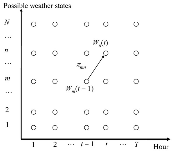
Figure 1.
A Markovian process.
The uncertain PV Generation is also a Markovian process, as follows:
where is the ideal PV generation at time n. The probability that the PV generation is at time t is the weighted summation of probabilities at time :
Generally, probabilities of PV levels at subsequent time-periods are obtained based on PV levels at previous time-periods and the transition matrix consisting of .
Tap changer. Assume that tap changers are associated with the corresponding solar farms. Following [15], and assuming that bus indices are omitted for brevity, tap-changer constraints are:
where is voltage input, a is a transformer-turn ratio under no-load conditions as: /, is transformer leakage impedance, generally a function of a, but here is assumed to be a complex number, and S is the transformer load. For mathematical expediency, (9) is equivalently written as:
The transformer turn ratios , which are decision variables, are controlled as:
where is the “rated turn ratio”, is the single tap position change, and are integer decision variables denoting tap positions as:
3.3. Inter-Nodal (Global) Constraints
AC Power Flow in Rectangular Coordinates. Following [17,18,19,20,21], AC power flows are modeled by using complex voltages as:
Here, is susceptance and is conductance of line . Node stands for a “sending” node, and stands for a “receiving” node of line l.
Nodal Power Flow Balance Constraints. For every PV state n and at every node b, the net “inflow” should be equal to the net “outflow”:
If bus b contains no generators, then (here, is a set of generators at bus b); if bus b contains no load, then = 0, and if there is no PV generation, then .
Line-Capacity Constraints. For every PV state n and every line l, power flows satisfy the following line-capacity constraints:
The above problem belongs to a class of Mixed-Integer Non-linear Programming problems notable for non-convexities brought by non-linear AC power flows as well as by discrete decision variables.
4. Solution Methodology
To solve the above problem, the methodology “-proximal” Surrogate Lagrangian Relaxation method [10] is extended to handle tap-changer and droop-control constraints. After linearizing the problem and relaxing nodal flow balance constraints, Lagrangian multipliers are updated based on constraint violations, and the violations are penalized using “absolute-value” penalties; to ensure overall feasibility “-proximal” terms are used.
4.1. Surrogate Absolute-Value Lagrangian Relaxation
Relaxed Problem. After relaxing nodal flow balance (15)–(16), and penalizing their violations, the relaxed problem becomes:
where are multipliers relaxing power flow balance constraints (16). The vector, denotes a vector of power flow balance constraint violations.
Following [10], multipliers are updated as:
where
where is defined as
In the beginning, is increased by a constant :
After constraint violations become zero, a feasible solution is obtained, and needs to decrease as:
Subsequently, the is not increased.
4.2. Practical Implementation
Voltage restrictions (4), droop control for voltage (6), tap-changer constraints (10), AC power flows (13) and (14), as well as line-capacity constraints (17) are non-linear. Moreover, the left-hand side constraint of (4) and (13) and (14) delineate non-convex regions. Following the work [10], these difficulties are briefly addressed next. The method of [10] is then extended to improve the linearization of (4) as well as to resolve non-linearity difficulties brought by the newly considered droop control (6) and tap-changer constraints (10).
In the following, the main linearization principles will be delineated first. Then, the feasibility will be established.
- 1.
- Linearization of Cross-Product Terms within (13) and (14). To linearize AC Power Flow while updating all the voltages, the following formula is used:Reactive power is linearized in the same fashion.
- 2.
- To avoid infeasibility along the iterative procedure, “soft" penalization is introduced through the non-negative penalty variables and as:To enforce the feasibility of (25), and are penalized.
- 3.
- Linearization of Tap-Changer Constraints (10). Tap-changer constraints contain both the cross-products and the squared terms. Following the ideas of above-presented linearization, the linearization is performed as follows:The linearization of line-capacity constraints (17) is operationalized in the same way as described in point 2 and 3 above.
- 4.
To ensure that solutions to the linearized problem satisfy the corresponding original (non-linear) problem terms , , and , which capture the deviations of voltages , linearized power flows and transformer turns ratios from previously obtained values are introduced and are penalized by . The intention here is to discourage oscillations of solutions while encouraging their approach to common values. To avoid getting trapped at previously obtained values, is chosen to be lower than .
Linearized Relaxed Problem.
The resulting MSO relaxed problem then becomes:
Multipliers are updated as in (18), with the difference that the vector of constraint violations is appended by and , and the vector of multipliers is appended by and . Multipliers corresponding to inequality constraints cannot be negative, and are projected onto a positive orthant. Piece-wise linear -norms within (28) are linearized by using standard special ordered sets [22,23].
Feasibility. As increases, violation levels of relaxed constraints decrease. However, the total lack of constraint violations does not imply feasibility because, for example, linearized power flows do not coincide with original power flows. To ensure that and , increases as in (21):
The intention here is to force “-proximal” terms to zero to ensure feasibility, after which is decreased as
After constraint violations and proximal terms are both zero, the feasible solution is obtained. Forcing the violations exactly to zero may require a considerable number of iterations, so tolerances and are introduced for constraint violations and proximal terms, respectively. The algorithm is shown in Algorithm 1 and the flow chart in shown in Figure 2 below.
| Algorithm 1 Surrogate Lagrangian Relaxation. |
Initialize , , and while stopping criteria are not satisfied 1 solve MSO problem 2 If the total constraints violations and total violation of proximal terms is update multipliers and increase c 3 If the total constraints violations and total violation of proximal terms is update multipliers, stop increasing c and increase 4 If the total constraints violations and total violation of proximal terms is reduce c and stop increasing |
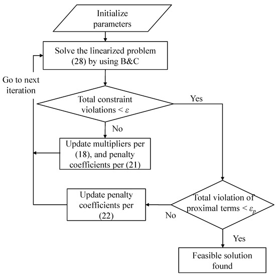
Figure 2.
Surrogate Lagrangian Relaxation.
Stopping Criteria. Within the above Algorithm, the “if” condition in step can by itself be used as a stopping criterion. Alternatively, after c is reduced per , the algorithm can continue with the multipliers update until a predefined CPU limit is reached.
5. Results
The method is implemented using IBM ILOG CPLEX Optimization Studio V 12.8.0.0 [24] on a PC with 2.40 GHz Intel Xeon E-2286M CPU and 32G RAM. To demonstrate the coordination aspect and the near-optimal performance of the method, a simple nine-bus system is considered.
5.1. System Description
Consider a nine-bus system with meshed topology as shown in Figure 3 below [25]. Assume that at buses 2 and 3 there is a generator, respectively; at bus 4 there is a solar farm of three stochastic states, and a tap changer; while at buses 5, 7, and 9, there is a load. The micro-grid is connected to the main grid through bus 1. The time interval is 15 min and the planning horizon is 3 h.
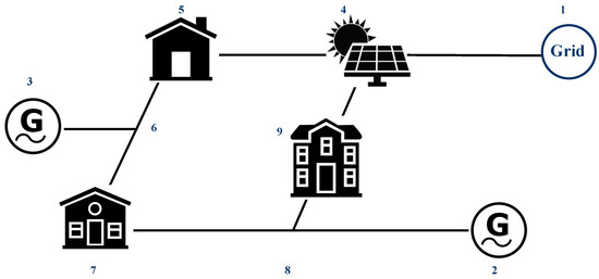
Figure 3.
Topology of the 9-bus system; bus numbers are labeled by using arabic numerals (1–9).
5.2. Results and Discussions
5.2.1. Droop Control
To demonstrate the performance of droop control, the micro-grid is disconnected from the grid at interval 12; thus turning the local operations into the islanded mode. By using the approach developed above, the problem (1)–(17) is solved, and a feasible solution is obtained in 202 seconds. The results show that the frequency stays within the range of [59 Hz, 61 Hz] due to effective droop control.
5.2.2. Tap-Changer
To show the impacts of tap changing, the problem in Section 5.2.1 is solved again without tap-change-related costs in the objective function. The results are compared in Table 1 below. It can be seen that the expected number of tap changes is greatly reduced when the corresponding cost is considered in the objective function.

Table 1.
Results on tap-changing.
5.2.3. Costs
To show the benefits of being connected to the main grid all the time, the problem in Section 5.2.1 is solved again under the grid-connected mode. The results are compared in Table 2 below. It can be seen that the total cost is reduced by connecting to the main grid, taking advantage of the time-varying costs of the grid power.
Table 2.
Results of two different grid-connection scenarios.
To provide insights into the convergence, the calculated trajectories of voltages at selected buses 2 and 5 at interval 12 are plotted on a complex plane in Figure 4. The feasible region delineated by constraints (4) is in-between and on the boundaries of the two concentric circles. Arrows schematically indicate the directions voltages move along to escape from infeasibility. It is demonstrated that voltages approach near-feasible solutions within a few iterations.
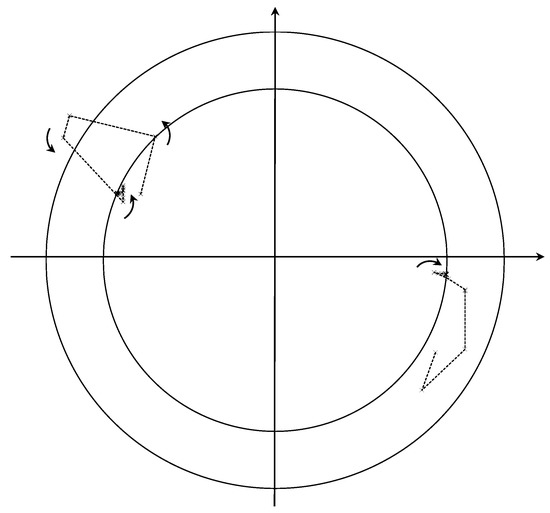
Figure 4.
Convergence of selected voltages at buses 2 and 5 at time period 12.
6. Conclusions
Motivation. Recent blackouts in California, New York, and Britain in 2019, which left millions of customers without power, pushed for an increase in the power system’s resilience, stability, and reliability. DERs, such as solar panels and wind turbines, have provided a promising solution. In order to prompt the applications of renewable energy or DERs, micro-grid is a promising paradigm. Informative Methodology. This paper addresses the issues of sustainability of micro-grid operations. Through the consideration of Markov processes to capture stochasticity of renewable generation; through tap-changer constraints penalizing frequent changes of taps, with which the lifespan of the expensive equipment will be greatly extended; through consideration of AC power-flow constraints appropriate for distribution systems; and through droop-control constraints for restoration of frequency and voltage after disconnection from the main grid. The above-mentioned constraints lead to non-convexities and difficulties solving the resulting micro-grid operation optimization problems. The methodology based on dynamic linearization and -norm penalization is exact and is amenable to the use of MILP solvers. After linearization, the only source of non-convexities is the presence of discrete variables, which are efficiently handled by MILP solvers. Key Results. It is demonstrated that voltages approach feasible values within a few iterations, leading to exact satisfaction of AC power flows ensuring the feasibility of operations. As a result of the above, the overall performance of the method leads to convergence within a matter of minutes. It is also demonstrated that micro-grid operations benefit from the new solution methodology; specifically, the number of tap changes is drastically reduced, thereby ensuring higher sustainability in the presence of voltage fluctuations caused by uncertainties. Main Advantages over Previous Studies. The main advantage over previous studies is the consideration of key elements that lead to the feasibility of sustainability of micro-grid operations; namely, exact AC power flow, droop control, and tap-changer constraints are considered without simplification, and the methodology ensures their exact satisfaction. Limitations and Challenges of the Experimental Study. When considering multiple micro-grids, PV (or wind) generation at different locations cannot be aggregated and has to be modeled as a Markov chain per PV bus. The resulting global states are a large number of combinations of nodal states, leading to much-increased complexity. Suggestions for Future Research. With an increase in the number of micro-grids, which are expected to be interconnected, it is suggested that the methodology is extended to coordinate several micro-grids; on the bright side, upon the decomposition inherent in the method developed, the micro-grid complexity associated with both the number of discrete variables and the number of stochastic states can be significantly reduced. The present work: 1. has enabled efficient resolution of micro-grid subproblems and 2. paves the way for efficient coordination of micro-grids. The coupling constraints that connect adjacent micro-grids can be dualized by the Surrogate Lagrangian Relaxation to efficiently coordinate micro-grids for high resilience and reliability spanning larger geographical areas.
Author Contributions
Conceptualization, P.Z.; methodology, M.A.B. and B.Y.; software, M.A.B., B.Y. and A.K.; validation, B.Y. and A.K.; investigation, M.A.B.; data curation, B.Y.; writing—original draft preparation, M.A.B., B.Y., A.K. and N.Y.; writing—review and editing, M.A.B., B.Y., A.K. and N.Y.; visualization, M.A.B. and B.Y.; supervision, P.Z.; project administration, P.Z., N.Y. and M.A.B.; funding acquisition, P.Z., M.A.B. and B.Y. All authors have read and agreed to the published version of the manuscript.
Funding
This work is supported in part by the National Science Foundation under the grant ECCS-1810108, CNS-2006828 and OIA-2134840.
Institutional Review Board Statement
Not applicable.
Informed Consent Statement
Not applicable.
Data Availability Statement
Not applicable.
Conflicts of Interest
The authors declare no conflict of interest.
Abbreviations
The following abbreviations are used in this manuscript:
| MILP | Mixed-Integer Linear Programming |
| MSO | Micro-grid system operator |
| OPF | Optimal Power Flow |
| PV | Photovoltaic |
| SOCR | Second-Order Cone Relaxation |
References
- Stott, B.; Jardim, J.; Alsac, O. DC power flow revisited. IEEE Trans. Power Syst. 2009, 24, 1290–1300. [Google Scholar] [CrossRef]
- Yeh, H.G.; Gayme, D.F.; Low, S.H. Adaptive var control for distribution circuits with photovoltaic generators. IEEE Trans. Power Syst. 2012, 27, 1656–1663. [Google Scholar] [CrossRef]
- Tan, S.; Xu, J.; Panda, S.K. Optimization of distribution network incorporating distributed generators: An integrated approach. IEEE Trans. Power Syst. 2013, 28, 2421–2432. [Google Scholar] [CrossRef]
- Liu, G.; Jiang, T.; Ollis, T.B.; Zhang, X.; Tomsovic, K. Distributed energy management for community microgrids considering network operational constraints and building thermal dynamics. Appl. Energy 2019, 239, 83–95. [Google Scholar] [CrossRef]
- Wang, Z.; Chen, H.; Wang, J.; Begovic, M. Inverter-less hybrid voltage/var control for distribution circuits with photovoltaic generators. IEEE Trans. Smart Grid 2014, 5, 2718–2728. [Google Scholar] [CrossRef]
- Farivar, M.; Low, S.H. Branch Flow Model: Relaxations and Convexification—Part I. IEEE Trans. Power Syst. 2013, 28, 2554–2564. [Google Scholar] [CrossRef]
- Torbaghan, S.S.; Suryanarayana, G.; Höschle, H.; D’hulst, R.; Geth, F.; Caerts, C.; Hertem, D.V. Optimal Flexibility Dispatch Problem Using Second-Order Cone Relaxation of AC Power Flows. IEEE Trans. Power Syst. 2020, 35, 98–108. [Google Scholar] [CrossRef]
- Heydt, G. The next generation of power distribution systems. IEEE Trans. Smart Grid 2010, 1, 225–235. [Google Scholar] [CrossRef]
- Li, Q.; Vittal, V. The convex hull of the AC power flow equations in rectangular coordinates. In Proceedings of the 2016 IEEE Power and Energy Society General Meeting (PESGM), Boston, MA, USA, 17 July 2016; pp. 1–5. [Google Scholar]
- Bragin, M.A.; Dvorkin, Y. TSO-DSO Operational Planning Coordination through “l1-Proximal” Surrogate Lagrangian Relaxation. IEEE Trans. Power Syst. 2022, 37, 1274–1285. [Google Scholar] [CrossRef]
- Guan, X.; Xu, Z.; Jia, Q. Energy-efficient buildings facilitated by microgrid. IEEE Trans. Smart Grid 2010, 1, 243–252. [Google Scholar] [CrossRef]
- Mohammadi, S.; Soleymani, S.; Mozafari, B. Scenario-based stochastic operation management of MicroGrid including Wind, Photovoltaic, Micro-Turbine, Fuel Cell and Energy Storage Devices. Electr. Power Energy Syst. 2014, 54, 1–7. [Google Scholar] [CrossRef]
- Luh, P.B.; Yu, Y.; Zhang, B.; Litvinov, E.; Zheng, T.; Zhao, F.; Zhao, J.; Wang, C. Grid integration of intermittent wind generation: A Markovian approach. IEEE Trans. Smart Grid 2014, 5, 732–741. [Google Scholar] [CrossRef]
- Yan, B.; Luh, P.B.; Warner, G.; Zhang, P. Operation Optimization for Microgrids with Renewables. IEEE Trans. Autom. Sci. Eng. 2017, 14, 573–585. [Google Scholar] [CrossRef]
- Kasztenny, B.; Rosolowski, E.; Izykowski, J.; Saha, M.M.; Hillstrom, B. Fuzzy logic controller for on-load transformer tap changer. IEEE Trans. Power Deliv. 1998, 13, 164–170. [Google Scholar] [CrossRef]
- Sokugawa, T.; Shawver, M. Big data for renewable integration at Hawaiian electric utilities. In Proceedings of the DistribuTech Conference & Exhibition, Orlando, FL, USA, 9–11 February 2016; pp. 9–11. [Google Scholar]
- Torres, G.L.; Quintana, V.H.; Lambert-Torres, G. Optimal Power Flow on Rectangular Form Via an Interior Point Method. In Proceedings of the 1996 IEEE North American Power Symposium, Boston, MA, USA, 10–12 November 1996. [Google Scholar] [CrossRef]
- da Costa, V.; Martins, N.; Pereira, J.L.R. Developments in the Newton Raphson Power Flow Formulation Based on Current Injections. IEEE Trans. Power Syst. 1999, 14, 1320–1326. [Google Scholar] [CrossRef]
- Zhang, X.P.; Petoussis, S.G.; Godfrey, K.R. Nonlinear Interior Point Optimal Power Flow Method Based on a Current Mismatch Formulation. IEEE Proc. Gener. Transm. Distrib. 2005, 152, 795–805. [Google Scholar] [CrossRef]
- Bai, X.; Wei, H.; Fujisawa, K.; Wang, Y. Semidefinite Programming for Optimal Power Flow problems. Int. J. Electr. Power Energy Syst. 2008, 30, 383–392. [Google Scholar] [CrossRef]
- Li, Q.; Yang, L.; Lin, S. Coordination Strategy for Decentralized Reactive Power Optimization Based on a Probing Mechanism. IEEE Trans. Power Syst. 2015, 30, 555–562. [Google Scholar] [CrossRef]
- Bragin, M.A.; Luh, P.B.; Yan, B.; Sun, X. A Scalable Solution Methodology for Mixed-Integer Linear Programming Problems Arising in Automation. IEEE Trans. Autom. Sci. Eng. 2019, 16, 531–541. [Google Scholar] [CrossRef]
- Sun, X.; Luh, P.B.; Bragin, M.A.; Chen, Y.; Wan, J.; Wang, F. A Novel Decomposition and Coordination Approach for Large-Scale Security Constrained Unit Commitment Problems with Combined Cycle Units. IEEE Trans. Power Syst. 2018, 33, 5297–5308. [Google Scholar] [CrossRef]
- IBM ILG CPLEX V 12.1 User’s Manual. Available online: https://www.ibm.com/docs/en/SSSA5P_12.8.0/ilog.odms.studio.help/pdf/usrcplex.pdf (accessed on 12 May 2022).
- Zimmerman, R.D.; Murillo-Sanchez, C.E. MATPOWER (Version 7.1) [Software]. 2020. Available online: https://matpower.org (accessed on 12 May 2022).
Publisher’s Note: MDPI stays neutral with regard to jurisdictional claims in published maps and institutional affiliations. |
© 2022 by the authors. Licensee MDPI, Basel, Switzerland. This article is an open access article distributed under the terms and conditions of the Creative Commons Attribution (CC BY) license (https://creativecommons.org/licenses/by/4.0/).