Abstract
Boosted interest in highly efficient power supplies based on renewables requires involving simulators during both the designing stage and the testing one. It is especially relevant for the power supplies that operate in the harsh environmental conditions of northern territories and alike. Modern solar panels based on polycrystalline Si and GaAs possess relatively high efficiency and energy output. To save designing time and cost, system developers use simulators for the solar panels coupled with the power converters that stabilize the output parameters and ensure the proper output power quality to supply autonomous objects: namely, private houses, small-power (up to 10 kW) industrial buildings, submersible pumps, and other equipment. It is crucial for the simulator to provide a valid solar panel I-V curve in various modes and under different ambient conditions: namely, the consumed power rating, temperature, solar irradiation, etc. This paper considers a solar panel simulator topology representing one of the state-of-the-art solutions. This solution is based on principles of classical control theory involving a pulse buck converter as an object of control. A mathematical model of the converter was developed. Its realization in MATLAB/Simulink confirmed the adequacy and applicability of both discrete and continuous forms of the model during the design stage. Families of I-V curves for a commercially available solar panel within the temperature range from to +25 C were simulated on the model. A prototype of the designed simulator has shown its correspondence to the model in Simulink. The developed simulator allows providing a full-scale simulation of solar panels in various operating modes with the maximum value of the open circuit voltage 60 V and that of the short circuit current 60 A. Issues of statistical processing of experimental data and cognitive visualization of the obtained curves involving the cognitive graphic tool 2-simplex have also been considered within the framework of this research. The simulator designed may serve as a basis for developing a product line of energy-efficient power supplies for autonomous objects based on renewables, including those operating in northern territories.
1. Introduction
The unprecedented penetration of renewables into low-voltage distribution grids originates full-scale R&D projects aimed at increasing the power output and investigating the control strategies for optimal power generation involving solar photovoltaic (PV) panels. In addition, the problem of greenhouse gas emissions is still up-to-date and needs to be attended [1].
An extensive body of literature [1,2,3,4] sheds light on the current trends in the area of renewable power generation. Solar panels have tremendous potential both as standalone electric power sources and within the hybrid power plants.
Over the last decade, the relevance of introducing renewables into generating capacities of power supplies has skyrocketed [2]. Moreover, per capita energy consumption is also on the rise [5]. Undoubtedly, this indicates the growth in technology and welfare in the countries that employ the potential of renewables according to governmental foundations, commercial programs, and grants [3]. Such countries as Kazakhstan, Uzbekistan, and Turkmenistan have huge territories with places where national power transmission lines are not provided. Those cites need stable power supply to be installed and maintained. The climate of these countries is severely continental. Even though the average temperature in winter there does not drop below −13 C, there are still cold places in the desert and mountains.
Another bunch of countries, namely, Canada, the USA, and Russia, have huge areas in the north where the problem of stable power supply is still valid. Surprisigly, such Russian regions as the Jewish Autonomous Region, Primorsky Kray, Altay Republic, and Irkutsk region are related to the Far North regions, even though they embrace the south of the country. This is due to the inherent climatic features of the above cites. Over 48% of the Canadian area is related to Northern Canada. In the USA, the American North and Alaska are the regions in which stable power supply for standalone facilites is not the least important.
The facilities include standalone buildings, meteorological stations, settlements for oil field workers, and others, where the total power rating of the energy-generating plants is around 100 kW.
Thus, providing stable power supply for autonomous objects in the places under discussion may inspire a fruitful R&D research concerning the introduction of solar panels into existing generating capacities. The most versatile approach for this purpose represents employing a hybrid power plant that include diesel, wind, and solar-generating units [6]. In these plants, the diesel generator represents a core component, whereas the other two are auxiliary ones. Nevertheless, the latter adds value to the overall power generating process by employing the potential of renewables, thus increasing the sustainability of the plant [5].
Extending this approach of combining the power supplies, we come to a micro-grid concept [7] that suggests an extensive application of additional energy sources and employing consumers to be producers of electricity that is injected into a utility grid.
The essentials of introducing PV-based sources into the power supplies of buildings is emphasized in [4]. This research considers the reduction in buildings’ energy consumption based on the concept of an all-electric nearly Zero-Energy Bulding (nZEB). The researchers actively implement mathematical modeling and simulation of the sources and emphasize that ‘a building’s performance during operation deviates from simulations’. Here, the term ‘simulations’ relates to exploring the performance of a power supply in a software environment. In the majority of cases, engineers have at their disposal operating power plants. Thus, there arises an issue of how to evaluate the introduction of a new solar panel into an existing operating power plant right on the spot. In this sense, both mathematical and simulation models are all-embracing tools of designing both standalone solar sources and their combination with diesel and wind units. Unfortunately, developing a model of the entire power plant takes a huge amount of time and cost. This gives us grounds to overcome the issue by developing a line of embeddable solar panel simulators that generate approximate I-V curves of the panels in all possible operating modes. Thus, the suggested simulators can be employed both in the designing stage and during the operation of energy-efficient power supplies.
The concept of an inverter-based grid-tied PV system is represented in [8]. The authors focus on connecting the PV system to the medium voltage grid through a multilevel cascaded inverter and investigating output power quality issues. Here, we observe a methodology based on modeling the proposed control technique in MATLAB Simulink and testing it with a reduced-scale prototype test platform, which can be attributed to a class of simulators.
Among the state-of-the-art solutions are the Solar Photovoltaic Array Simulation Solution for inverter-based solar power supplies [9] and a line of solar PV panel simulators for ground testing the power sources of satellites provided by Keysight Technologies [10]. These simulators provide high response characteristics, and their power rating reaches 30 kW.
Having analyzed the current trends in developing such sorts of simulators, we have undertaken research directed at providing the proper power supply of civil autonomous objects by simulating I-V curves analogous to that of the real solar panels in a wide temperature range. The said simulation may be carried out either in a lab or directly on the object.
In this paper, we focus on creating the methodology of designing such a class of devices and implementing them to introduce new power-generating capacities to the standalone small power plants that are supposed to be placed in the north territories.
Such plants may contain a set of diesel generators (2–3) coupled with wind-generating installations and solar panels. Such a power unit combination not only employs more generating potential but also allows ensuring power stability in the majority of operating modes ranging from no load to 10 or even 15% overload for a short time. Unfortunately, the price of diesel fuel is rather high primarily due to the costs on its transportation to the sites where power supplies are installed. Thus, employing hybrid power-generating complexes allows saving diesel fuel by switching off the diesel part when either wind speed or solar radiation are high enough to provide stable power supply for the consumers.
On the other hand, by implementing this method, we face the reliability issues involving such statistical parameters as failure rate and admissible number of commutations per unit time. Therefore, we are forced to constantly search for a trade-off between all the issues given in this paragraph. However, the high potential of employing solar PV panels to ensure stable power supply for autonomous objects gives us optimism in developing corresponding simulators.
In this paper, we suggest a structure of a solar PV panel simulator producing appropriate I-V curves for the panels employed primarily in the northern territories of the countries considered above. The core component of this simulator is a buck converter with a go-around loop and a current feedback. The device is supposed to be used on both the designing stage and the implementation one. The latter implies embedding the device into a real power-generating set to test the way the real PV panel would work both as a standalone power supply and within a hybrid power plant.
The paper is organized as follows. Section 2 clarifies the issues of designing and mathematical modeling of the simulator based on a buck converter topology. Section 3 delves into the simulation of the device in a MATLAB/Simulink software environment and considers the processing of digital experimental results. Experimental studies of the simulator prototype are presented in Section 4. Section 5 involves cognitive graphics to render the simulated curves in cognitive graphic tool 2-simplex. The results of the paper are analyzed and discussed in Section 6. Section 7 summarizes the research.
2. Designing and Mathematical Modeling of Solar Photovoltaic Simulator
In this section, we delve into the circuitry essentials of the simulator under development and the creation of its mathematical model.
Taking inspiration from [11], we borrowed some features from the paradigm of modeling and simulation framework for the Cyber-Physical Electrical Energy Systems based on open-source standard SystemC-AMS for creating a prototype of the simulator under design. The said framework serves as a tool for designing, simulating, and optimizing the processes of generation, distribution, storage, and consumption of energy involving sustainable power sources. Thus, we implemented the idea of a concurrent model developing in both the Electrical Linear Network (ELN) and Linear Signal Flow (LSF) domains to verify the correctness of the circuitry operation and derived mathematical model behavior. Moreover, the simulator may contribute to the physical domain of the framework realizing solar panel voltages and currents as values obtained from the sensors without using any equations.
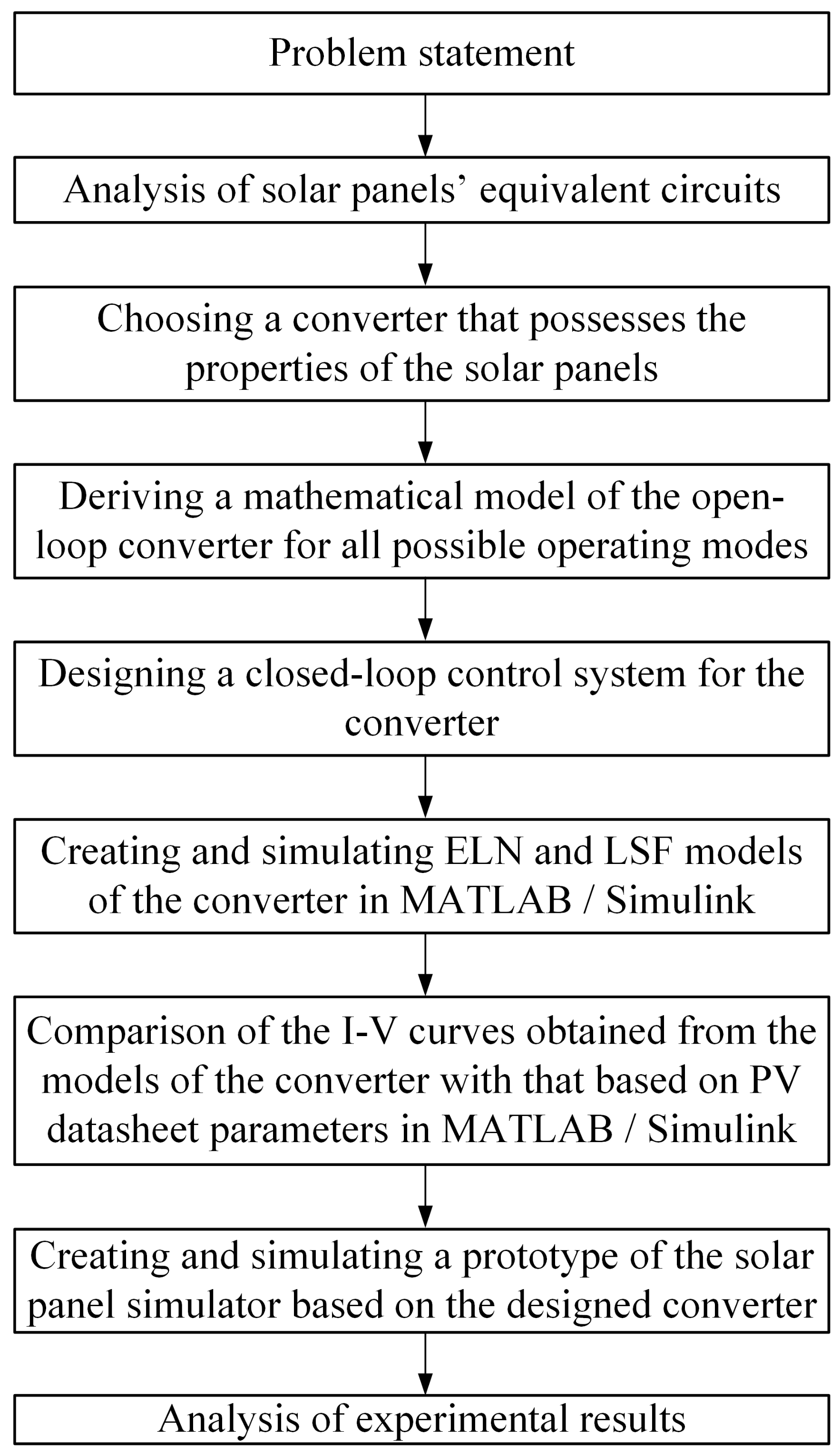
The concept serving as a backbone of the current research as a number of consecutive steps is represented in Figure 1.
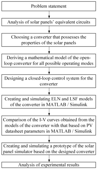
Figure 1.
Concept of simulator designing.
To back up our reasoning, we demonstrate the conventional equivalent circuits of an abstract electric power source and a solar cell in Figure 2.
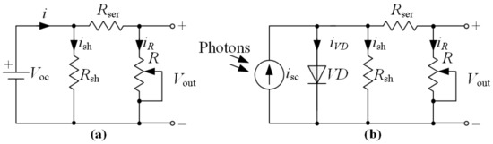
Figure 2.
Equivalent circuits of an abstract power source (a) and a solar cell (b).
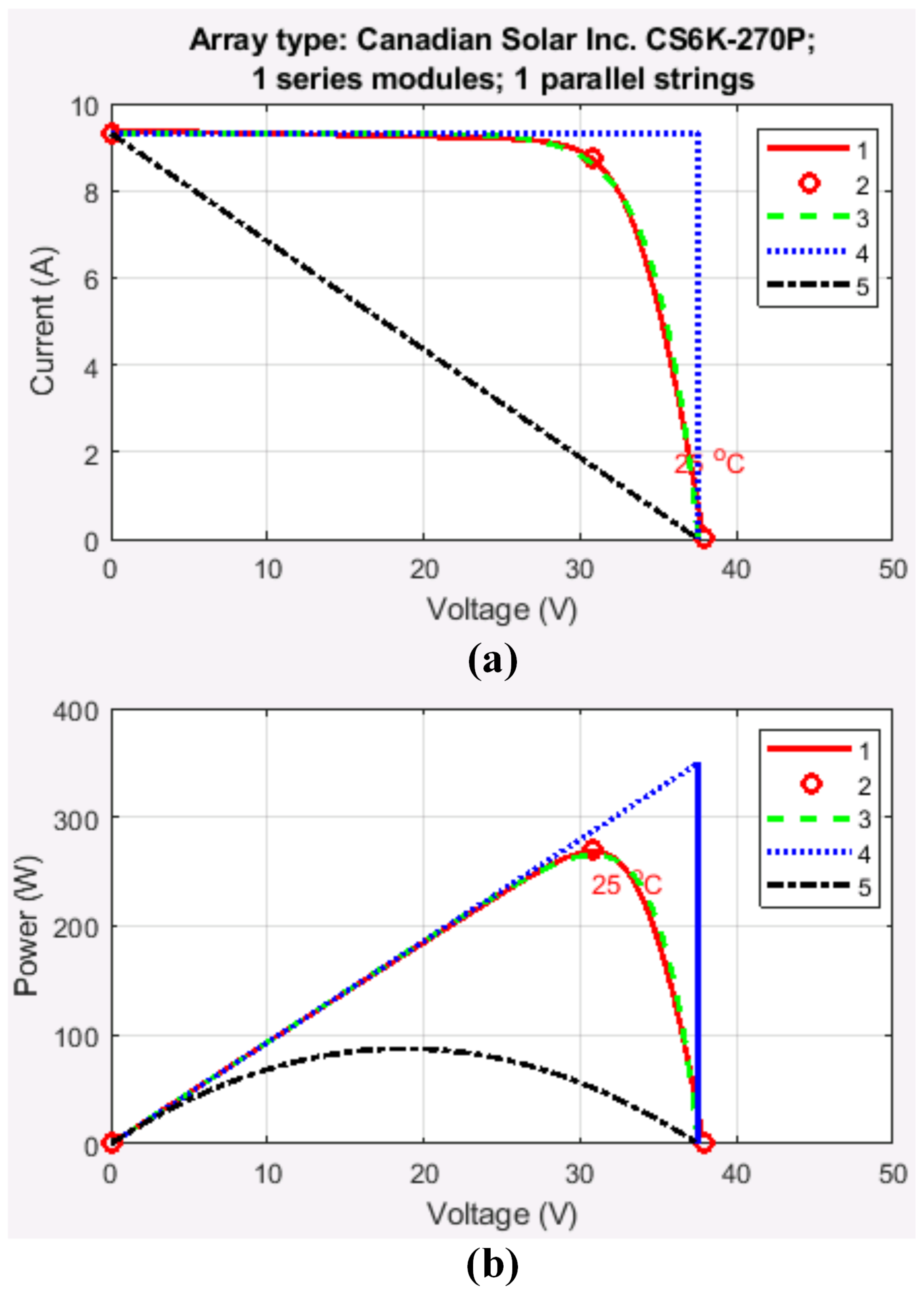
The serendipity behind the designing process lies in analyzing the essential features of these equivalent circuits and employing them into a converter topology that might possess these features. The common elements of the circuits (Figure 3) are shunt resistance , series resistance , and load one R. They completely define the I-V curve slopes on both current and voltage regions provided by the converter. As an object of simulation, we adopted a commercially available solar panel CS6K-270P [12]. This panel is presented in MATLAB 2021a Simulink in two libraries, namely Simscape → Electrical → Specialized Power Systems → Sources and Simscape → Electrical → Sources. The first library is related to the power components of electric circuits, whereas the second one corresponds to the so-called spice circuits [13] realized in Simulink. Both libraries represent the ELN domain. Generally, both models of the solar panel give the same characteristics, but the spice model of the PV cell allows obtaining the I-V curves at temperatures below 0 C. These curves serve as reference ones for comparison with those obtained with the simulator to be designed.

Figure 3.
Typical characteristics of power supplies: (a) current versus voltage; (b) power versus voltage. 1—I-V curve of panel CS6K-270P in Simulink power domain; 2—key points, namely the short circuit current, the maximum power point, and the open circuit voltage; 3—I-V curve of the panel in Simulink spice domain; 4—I-V curve of an ideal stabilized source; 5—I-V curve of a resistor.
The device under design is supposed to provide a family of I-V curves, the typical of which is shown in Figure 3. We also demonstrate in this figure characteristics of an ideal power supply and that of a resistor to emphasize the possible region of existence of solar I-V curves under given ambient conditions.
Characteristics 1 and 3 were acquired for solar irradiance and temperature 25 C. Under these conditions, the key point values are: short circuit current ; open circuit voltage ; current at maximum power point ; voltage at the said point ; maximum power .
Figure 3 indicates that the two solar PV panel models correspond to each other. Thus, we take the Simulink spice model with the datasheet parameters as a basis of our subsequent research.
Characteristics 4 and 5 are plotted to limit the region where the I-V curves may be located for a given irradiance and temperature. The series resistance corresponding to circuit (Figure 2a) and characteristic 5 (Figure 3) can be calculated as:
If we use a converter simulating characteristic 4, it usually requires two control loops to stabilize the current and voltage on the corresponding intervals. Still, this form of I-V curve is sometimes suitable to perform ground testing of space equipment in a so-called fixed mode [10].
The real I-V curve (Figure 3) is a nonlinear characteristic. We traditionally subdivide it into the three regions: namely, the current region where the current is practically constant, the transient one, and the voltage region where the voltage varies slightly. To realize nonlinearities in I-V curves, designers employ data tables generated from a set of analytical models [6,14,15,16,17,18]. In this paper, we do not use such tables relying on the suggested converter capabilities.
The basis of most of the PV panel models lies in an analytical model of a solar cell [14]. A common equation that determines a solar cell I-V curve can be written as:
where I is the load current of the solar cell; is the short circuit current also referred to as the photocurrent; is the reverse saturation current of diode ; is the Coulomb constant; V is the output voltage of the cell; is the Boltzmann constant; T is the operating temperature in Kelvin; is the series resistance of the solar cell; is its shunt resistance; and A is an empirical coefficient of the I-V curve, which is found by comparing a theoretical I-V curve and an experimental one of the solar cell.
As an alternative to this analytical model, we may also implement a semi-empirical model of a PV module [19] that relies only on datasheet information. This approach allows us to take into account the partial shading phenomena when modeling a solar PV panel operation.
Within the framework of this research, we used a MATLAB Simulink model based on datasheet information to determine the three key points of an I-V curve. We also assume that the solar panel simulator is supposed to generate an I-V curve passing through these points.
The topology of the simulator based on a buck converter illustrated in Figure 4 possesses a short circuit loop analogous to that of a conventional equivalent circuit (Figure 2b).
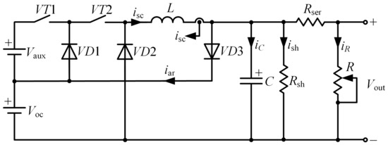
Figure 4.
Solar panel simulator topology.
All circuit parameters are calculated so as to provide a continuous conduction mode of the device. To ensure this, we rely on the fundamentals of power converters design [20] as well as on our previous results [21,22]: in this case, inductance and capacitance . At the input, we apply two stabilized voltage sources, namely, and .
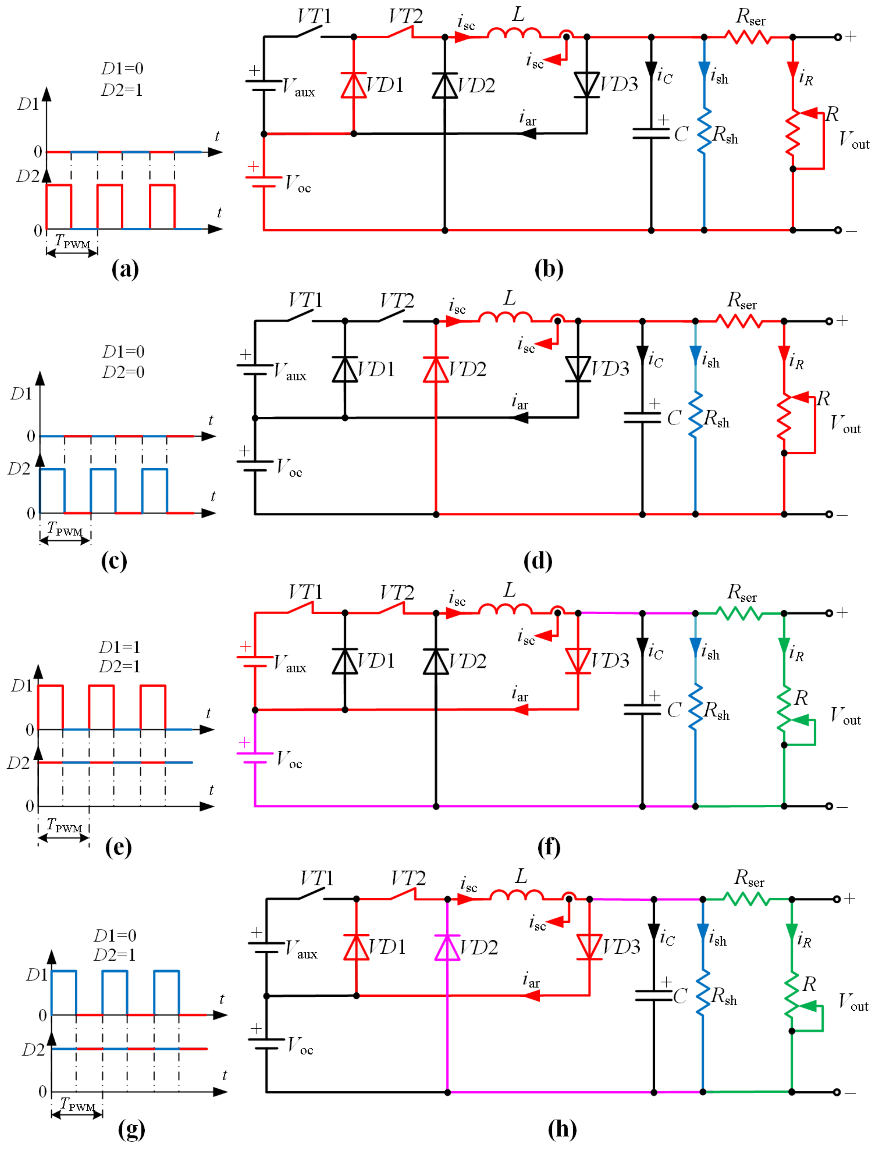
To clarify the principle of operation of this topology and to derive its mathematical model, we demonstrate a set of circuits corresponding to all possible states of transistors and (Figure 5).
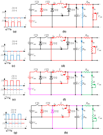
Figure 5.
States of the buck converter switches (a,c,e,g) and corresponding states of the circuit (b,d,f,h).
In this figure, each red waveform interval corresponds to a state of the circuit to the left. The color of the branches of the circuit state diagram correspond to the paths of current flow. The warmer the branch color, the higher the current flowing in it. When the slider of the variable load resistor R is at its top, the operating mode is close to a short circuit. When it is at the bottom, we deal with nearly an open circuit.
When the simulator operates in a steady-state mode within the current region, is always , whereas is PWM controlled (Figure 5a).
- ;
- .
If the steady-state operating mode of the simulator is rather close to short circuit, then the current flows through one loop:
- .
During transients, one more loop of charging the capacitance is formed in the following way:
- .
For this state, a set of Kirchoff’s equations takes the form:
- ;
- .
For the mode close to a short circuit, the current loop is as follows:
- .
Within the transient response interval, capacitor C charges through the loop:
- .
For this state, the equations are as follows:
For the voltage region, is always , whereas is PWM controlled.
When both switches are on (Figure 5e), the current loops in the steady state are as follows (Figure 5f):
- ;
- ;
- .
For the no-load condition, only the following two loops are valid:
- ;
- .
The capacitance charging loop in dynamics is given below:
- .
A set of equations describing electromagnetic processes within the interval under consideration can be written as:
Finally, when is (Figure 5g) within the voltage region, the current loops are formed as (Figure 5h):
- ;
- ;
- .
In no-load mode, the two current loops are:
- ;
- .
The capacitance charging loop in this case:
- .
The system of equations for the considered interval corresponds to (2).
Analyzing sets of Equations (2)–(4) and adding the limiting condition for the output voltage that must be stabilized at level within the voltage region, we derive a general set of equations that describes the behavior of the converter in all possible operating modes:
This versatile model allows considering duty ratios and either as continuous signals or discrete ones, thus obtaining a continuous or discrete simulator model, correspondingly. This approach was considered in detail in [21] for a boost converter topology. We accept the derived mathematical model (5) to realize it in MATLAB Simulink.
3. Simulation
In this section, we demonstrate MATLAB Simulink models corresponding to ELN circuitry (Figure 2a) and an LSN mathematical model (5) in its discrete (Figure 2b) and continuous interpretations.
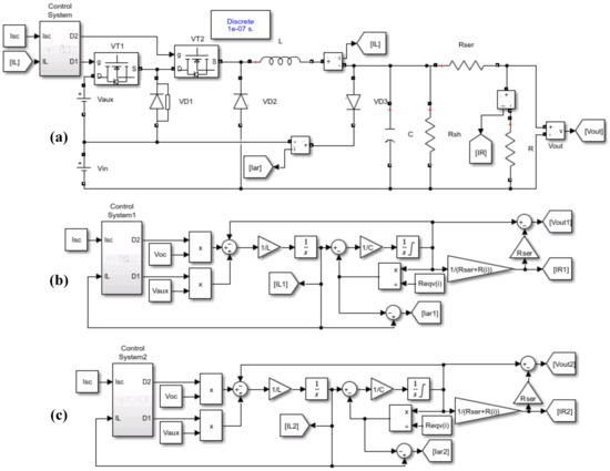
Figure 6.
Simulator models: (a) model in Specialized Power Systems domain; (b) discrete block diagram model; (c) continuous block diagram model. 1e-07 = 1 × 10.
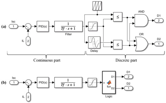
Figure 7.
Control system of the solar simulator: (a) discrete option; (b) continuous option.
In its turn, we subdivided the digital control system (Figure 6a) into a continuous part and a discrete one. The first one includes a PID controller acting so as to mitigate the error being the difference between the reference short circuit current and its actual value . An aperiodic filter is optional and serves to lower the PID output signal ripple. The filter output is limited within the range from 0 to 1. Then, this signal is compared to a sawtooth with a frequency of 25 kHz and its delay by a half of period. This is accomplished by relational operators. Then, the comparison resulting signals through the logical operators form control pulses and for transistors and , correspondingly.
For the continuous option of the control system (Figure 6c), the logic block is realized through MATLAB code (Appendix B). In this case, values and represent continuous functions of input u being the output of the PID controller output filter. The controller is automatically tuned in MATLAB Simulink with the following parameters: , , . Other methods of optimal controller tuning for electrical converters are outlined in [21,22,23]. These methods require a continuous transfer function of a converter to be derived and used as the open loop function. Then, this transfer function is reduced to a desirable open circuit one. The latter provides required quality criteria of the closed loop structure: namely, response time, overshooting, bandwidth, and others.
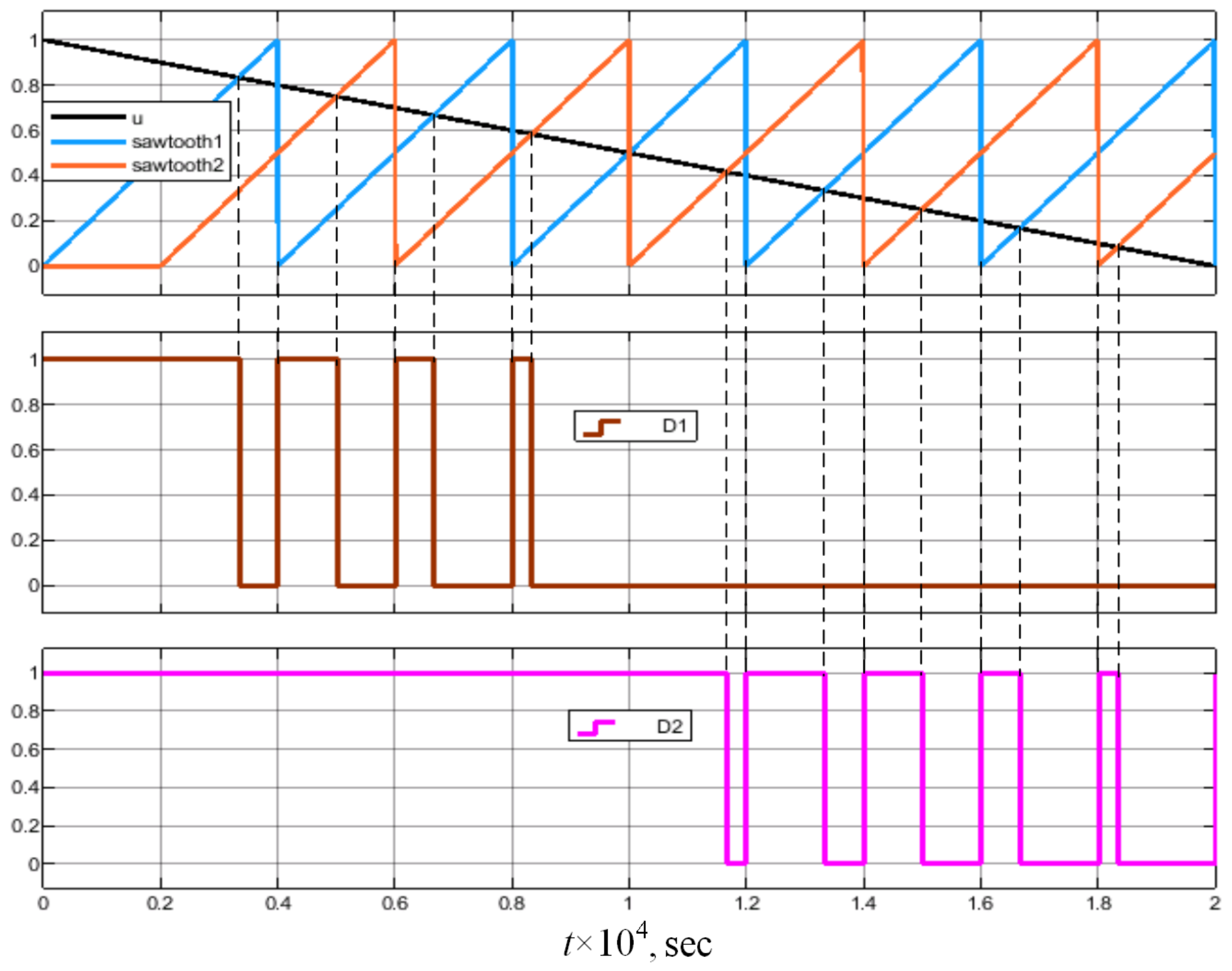
Figure 8 illustrates the waveforms of the input and output signals of the logical part.
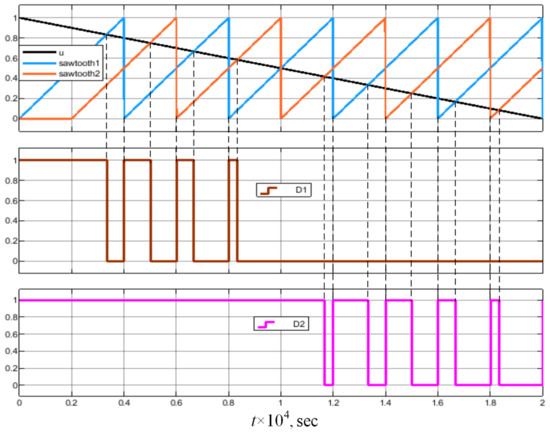
Figure 8.
Waveforms of the logical part of the control system.
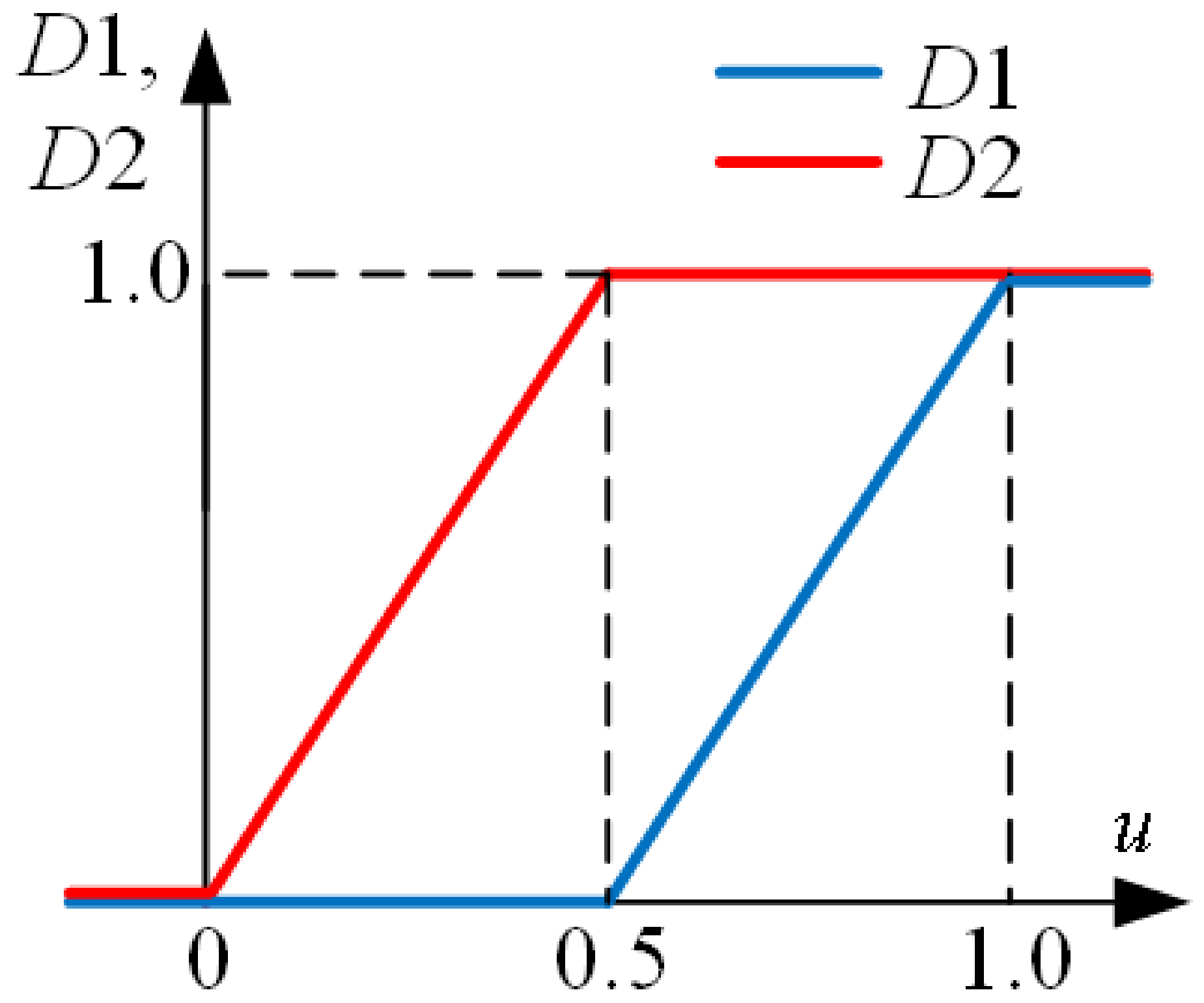
The corresponding control characteristics and realized by the logical part are depicted in Figure 9. Here, value u is an input signal for the logical block.
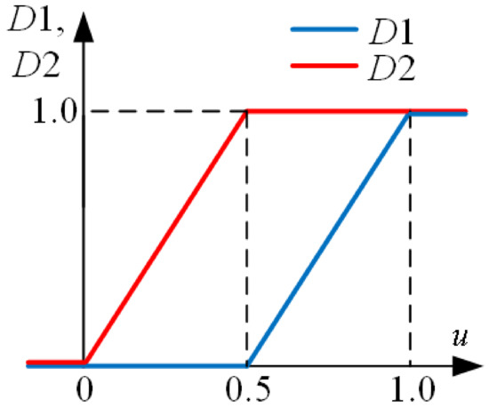
Figure 9.
Control characteristic of the solar panel simulator.
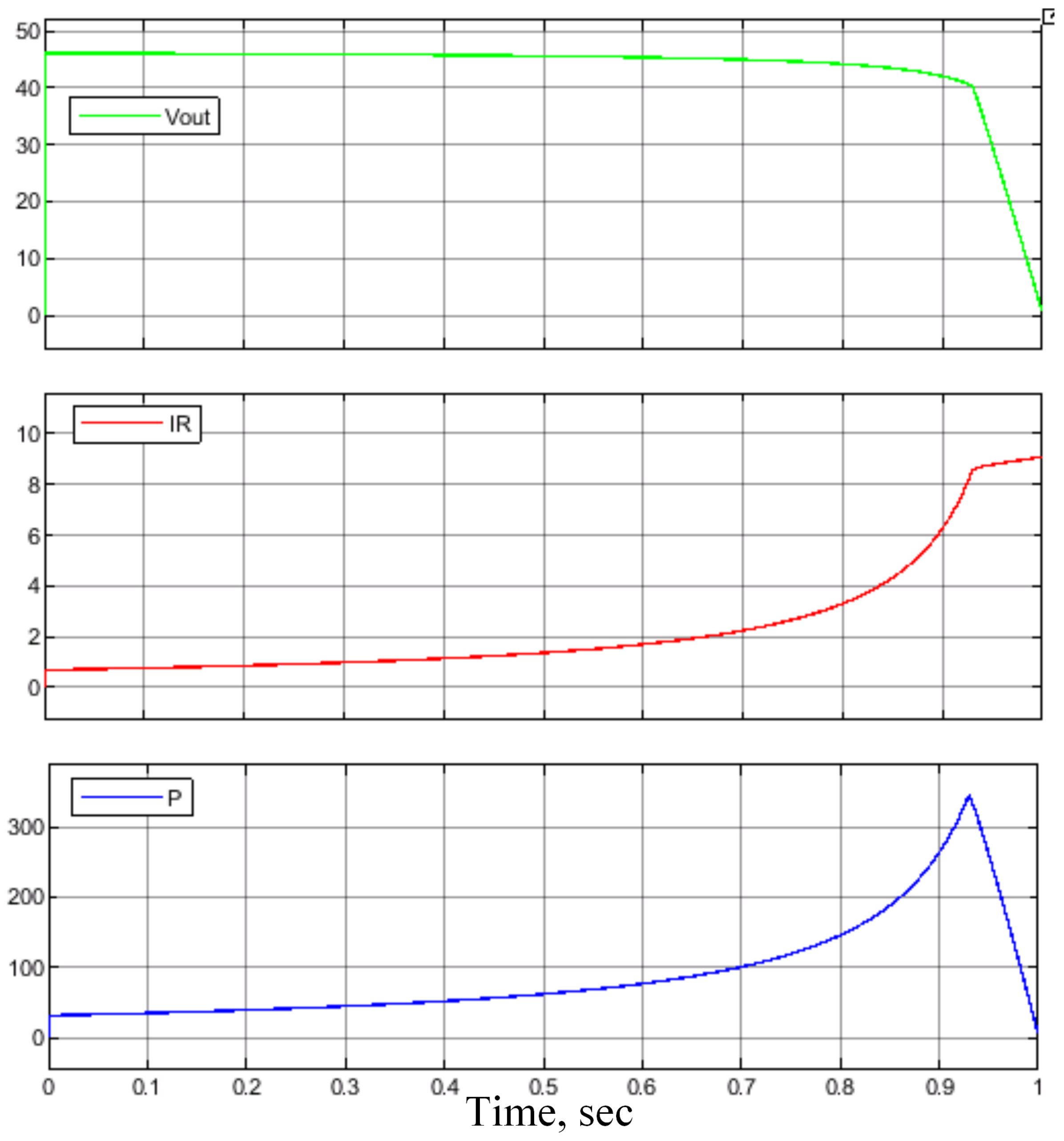
We emphasize that all the developed models Figure 6 give the same results. Figure 10 shows the dynamic characteristics of modeling solar panel CS6K-270P under conditions: and temperature −40 C. In this case, key points are: , , , , and external parameters , . Load resistance R varies linearly in time from 66.67 to 0.05 per 1 s symbolizing a gradual increase of the electric load.
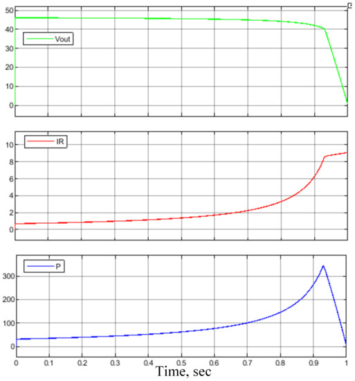
Figure 10.
Dynamic responses of the solar panel simulator.
At a time of approximately 0.93 s, the system changes its behavior, indicating the transition from the voltage to current region of the I-V curve.
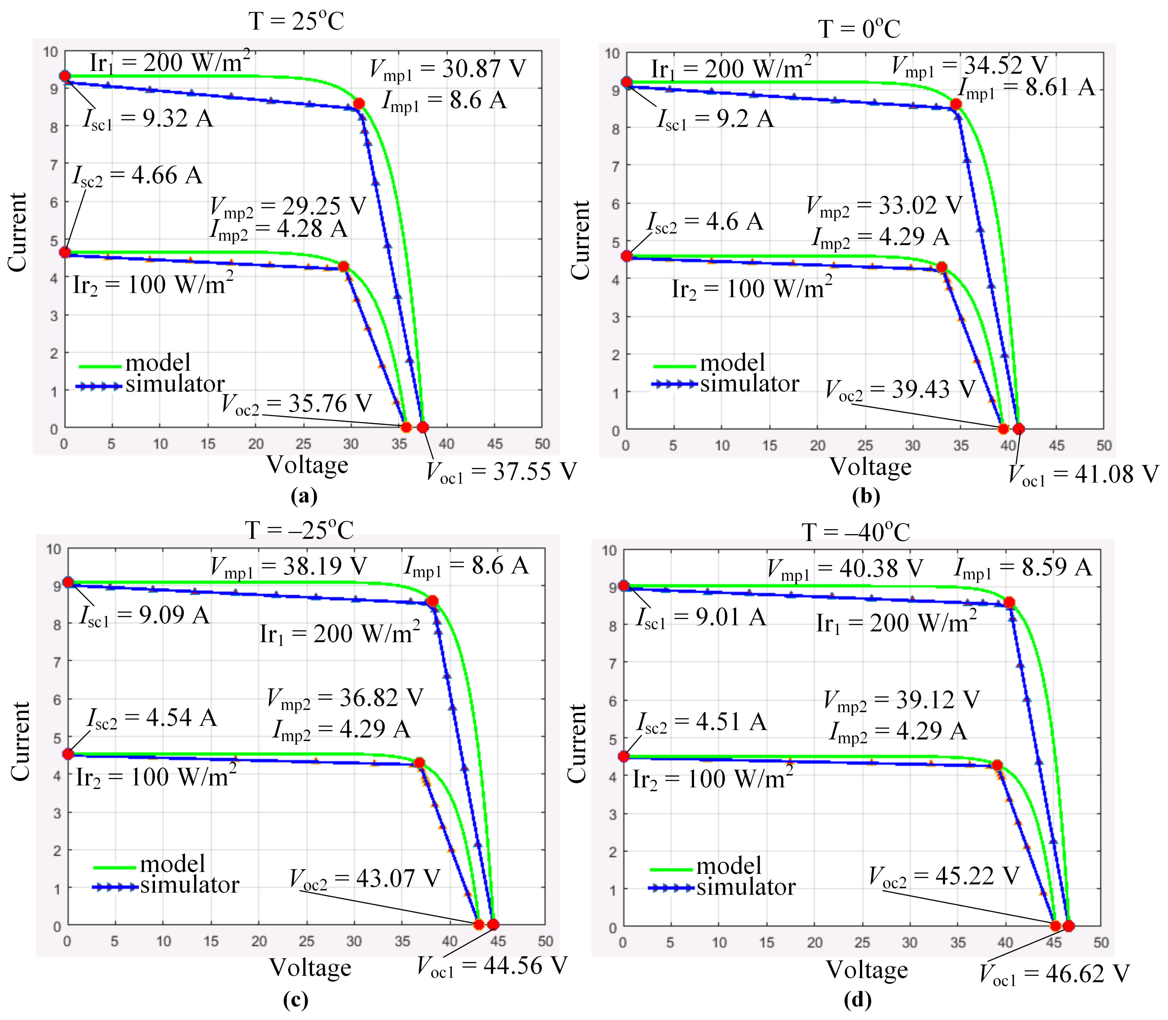
Families of I-V curves for the panel under consideration for various ambient conditions are shown in Figure 11.
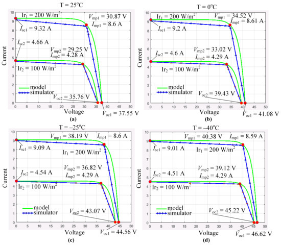
Figure 11.
Families of I-V curves provided by the solar panel simulator for temperatures (a) C; (b) C; (c) C; (d) C.
Observing these characteristics, we conclude that all the key points are properly reproduced by the developed simulator. Table 1 shows the major parameters of the simulated curves (Figure 11).

Table 1.
Data table for 2-simplex.
The standard deviations for the current and voltage regions were calculated according to the following equation [24]:
where is the sample of current or voltage array for the corresponding region, is the sample mean, and n is the corresponding array dimension.
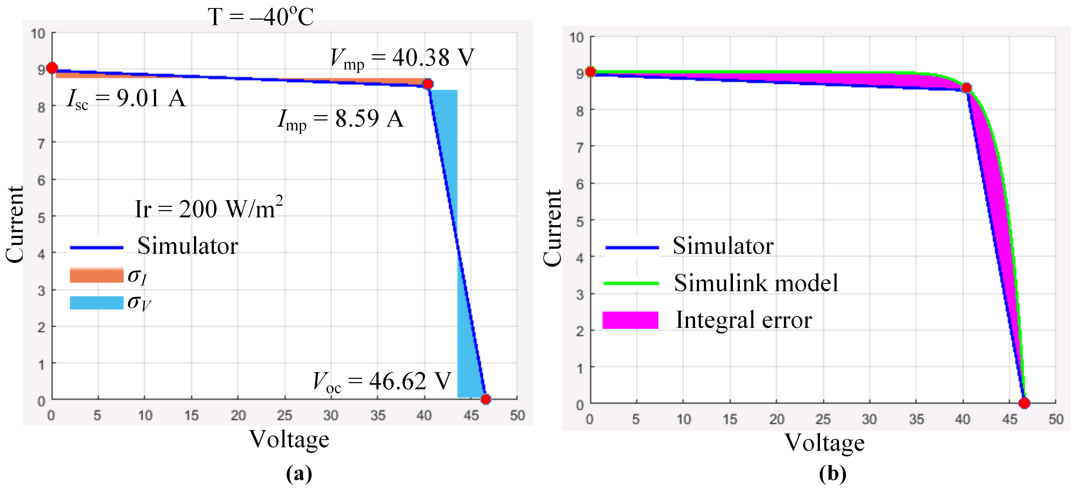
Standard deviations and for each point of the I-V curve are portrayed in Figure 12a in the form of colored areas.

Figure 12.
Rendering the standard deviations (a) and integral error (b) on I-V curves.
Integral error has been found as the difference of areas of a datasheet I-V curve and a simulated one, as illustrated in Figure 12b. To paint the areas, we implemented an original MATLAB code [25].
The corresponding formula for calculating the integral error is as follows:
where is the I-V curve obtained from the Simulink model with datasheet parameters, and is the I-V curve obtained from the simulator model.
Thus, simulation results demonstrate that the mathematical model (5) along with the models in MATLAB Simulink (Figure 6) can be implemented to develop a prototype of the solar panel I-V curve simulator.
4. Experimental Studies
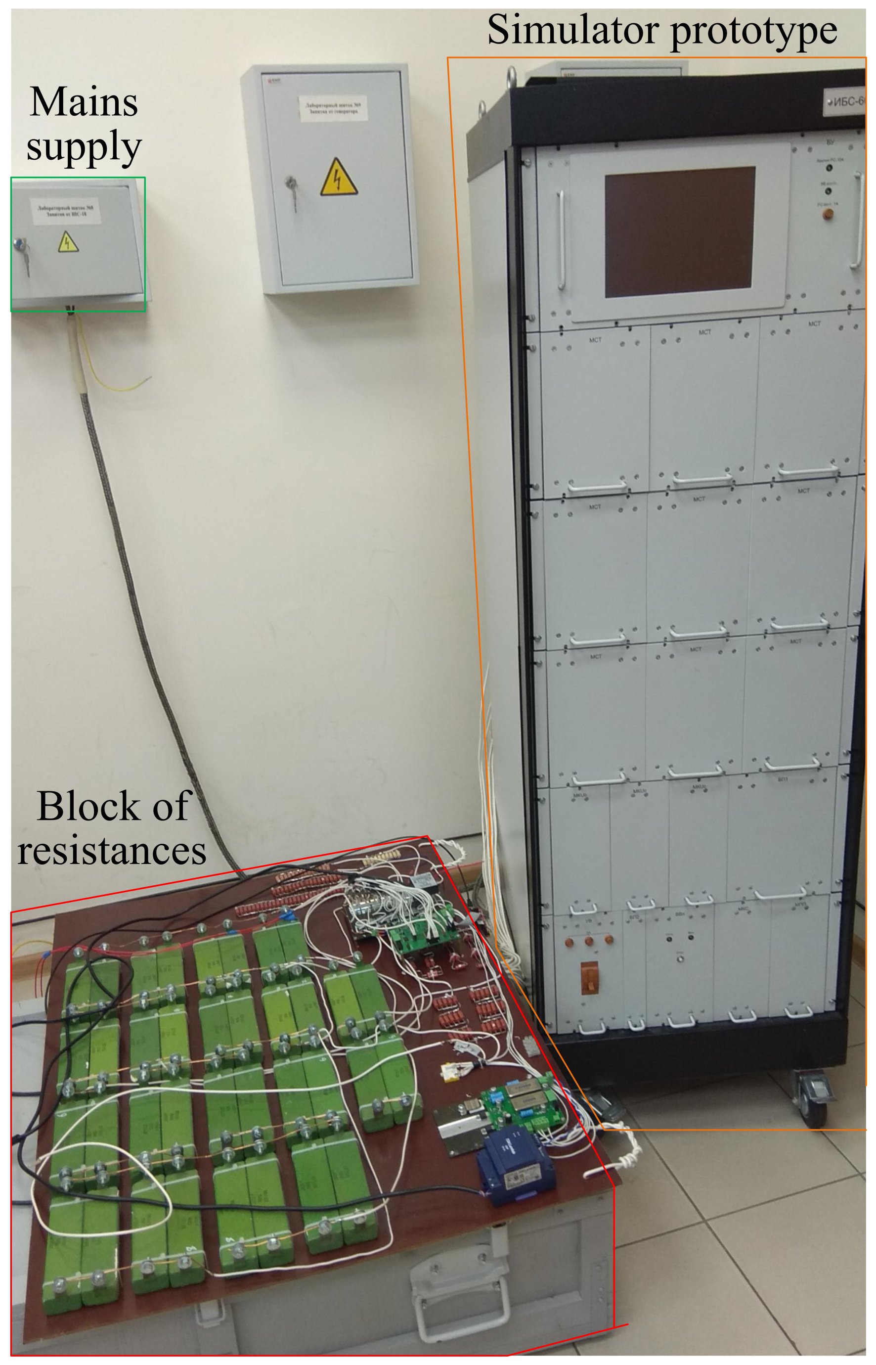
This section illustrates the experimental studies of the solar panel simulator prototype. The exterior of an experimental test bench is represented in Figure 13.

Figure 13.
Experimental test bench.
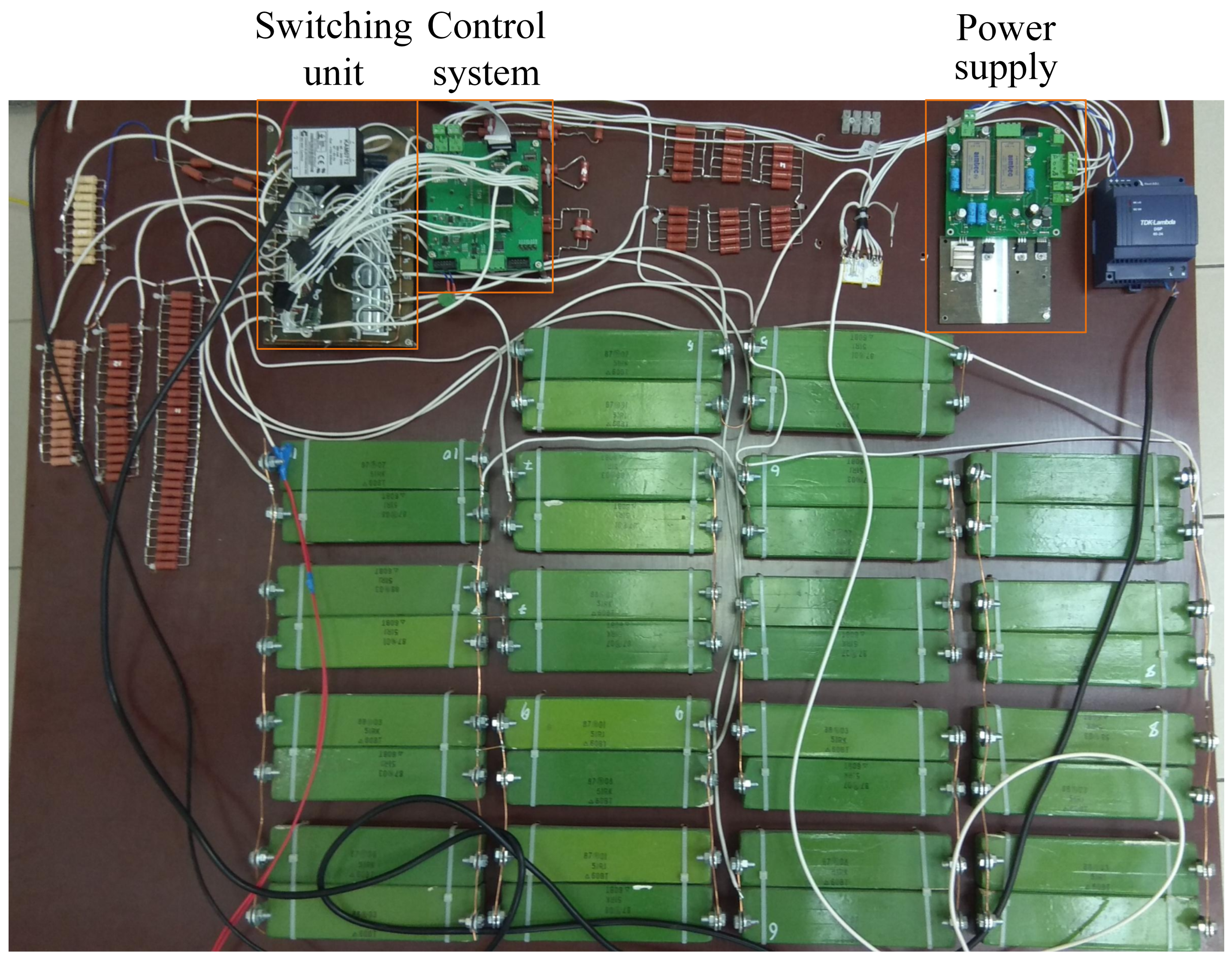
The curves were acquired with the following measuring set: oscilloscope LeCroy HDO4024AR with bandwidth 200 MHz and sampling frequency 2.5 MHz; current probe Tektronix TCP312A; current signal amplifier Tektronix TCPA300 with bandwidth 100 MHz and maximum current 30 A. The number of points of each curve equals 490. This number corresponds to the number of states provided by the block of resistances with its own power supply, control system, and switching unit. The front view of the block under consideration is shown in Figure 14.
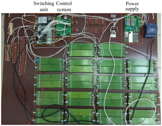
Figure 14.
Block of resistances.
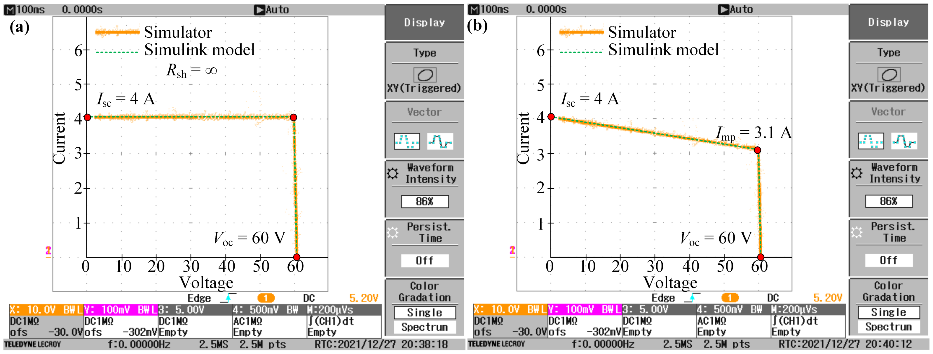
The simulated I-V curves are depicted in Figure 15. On each curve we also provided the corresponding characteristics obtained on the MATLAB Simulink model for comparison. An ideal I-V curve corresponds to and (Figure 15a). At the current stage of simulator designing, we introduced only shunt resistance , determining the slope of the current region as it is shown in Figure 15b. The voltage region in this case is represented by a vertical line segment, since .
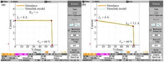
Figure 15.
Experimental I-V curves obtained on the simulator and its MATLAB Simulink model for shunt resistances (a) ; (b) .
Comparing the resulting I-V curves obtained from the simulator model and its prototype, we may conclude that they match with an admissible error.
5. Cognitive Graphics
Visualizing I-V curves and power versus voltage curves represents an inherent part of software for the solar panel simulators [9]. To render the operating point of the solar panel, we suggest to apply a tool known in literature as cognitive graphic tool 2-simplex [26]. This tool was extensively applied in a number of intelligent systems primarily designed for decision making and its justification. The fields of application include medicine, road building, oil engineering, electric power engineering, education, and others. The mathematical basis of cognitive graphic tools is thoroughly explained in a thesis [27]. Some essentials concerning the 2-simplex are demonstrated in Appendix A.
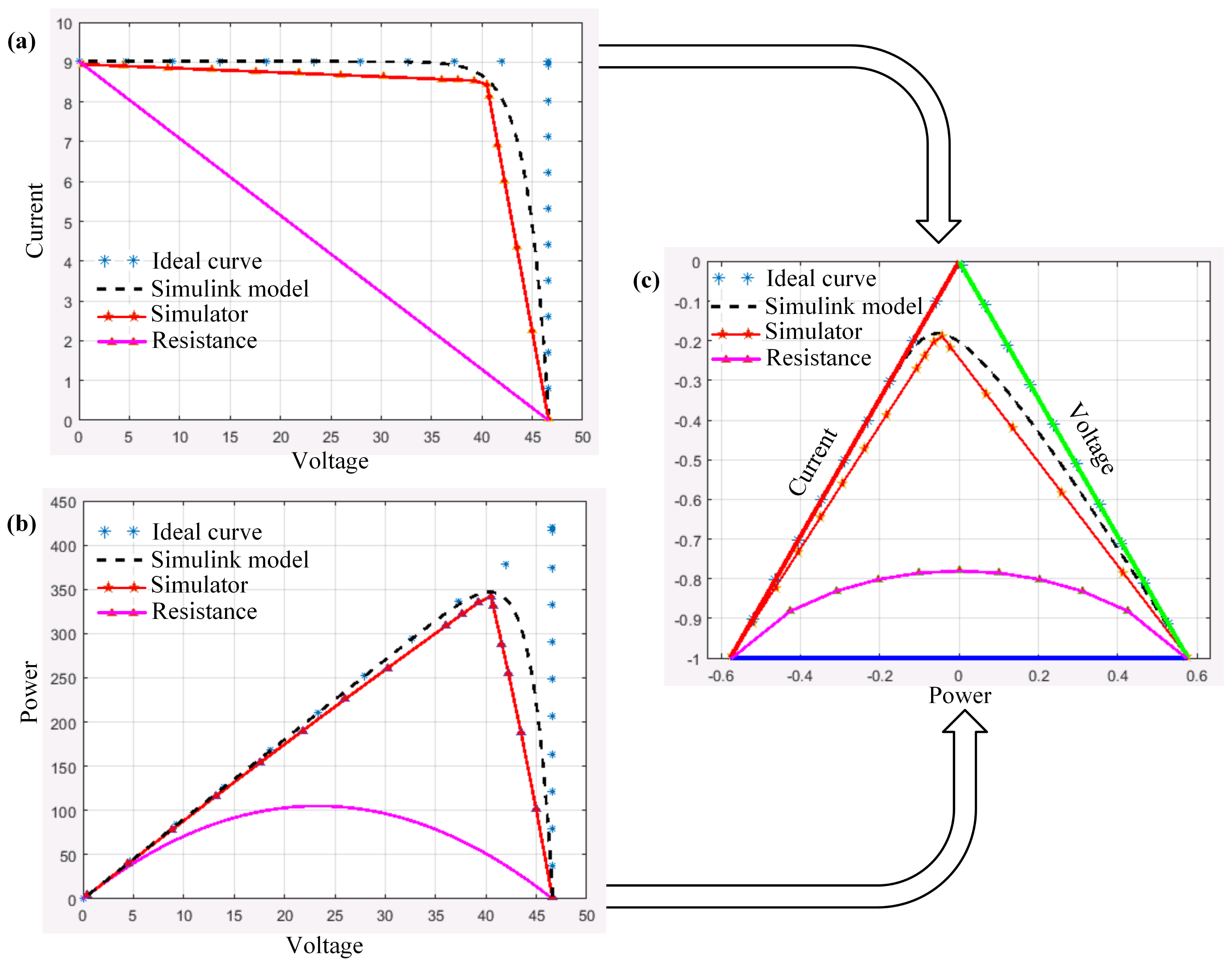
In this paper, we suggest using the 2-simplex to render the characteristics of a Simulink solar panel model and a family of others: namely, the simulated curves, the characteristics of an ideal power source, and that of a resistor. The idea is to combine such coordinates as current, voltage, and power in one 2D reference frame. For this purpose, we represent the I-V curves and power versus voltage curves for solar panel CS6K-270P [12] under conditions , C (Figure 16a,b). As a result, we demonstrate the obtained characteristics in Figure 16c.
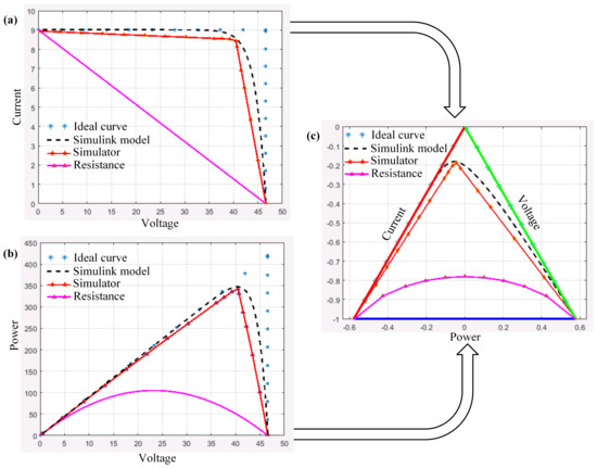
Figure 16.
Visualizing the curves (a) Current versus Voltage curve; (b) Power versus Voltage curve; (c) Power versus Current versus Voltage curve in 2-simplex.
In this figure, the triangle sides called ‘Current’, ‘Voltage’, and ‘Power’ constitute a 2-simplex. The distance measured by the length of a perpendicular from each of the curve points to sides ‘Current’ and ‘Voltage’ is directly proportional to the proximity to these values. This means that the closer the point is to the side, the greater the value of the corresponding variable (current or voltage). The length of the perpendicular to side ‘Power’ characterizes the normalized value of the solar panel power. The greater the length, the greater the power value.
The 2-simplex visualization allows cognitive rendering the power curves and observing the three variables in a 2D reference frame. This may serve as a basis for developing a human–machine interface for the simulator prototype.
6. Discussion
Experimental studies and cognitive rendering of the obtained characteristics show that the developed simulator can be implemented for designing power supplies with solar panels in their structure. For the accepted solar panel CS6K-270P, the device allows simulating I-V characteristics within the operating temperature range from −40 to 85 C [10]. This gives us grounds to assume that any other panel can be simulated within wide ranges of irradiance and temperature. These ranges are limited by short circuit current and open circuit voltage . Unfortunately, the designed simulator configuration cannot model a solar panel array involving bypass diodes for each of the PV substrings. This issue is thoroughly addressed in [19]. The authors proposed an original semi-empirical model of PV modules that takes into account the information about bypass diodes. In its turn, this approach allows realizing the PV array operation under partial shading that is crucial not only for civil applications but also for a number of space systems. Thus, to realize all these options by the simulator under discussion, we might need to employ one more control loop for the output voltage along with implementing more simulators with bypass diodes in one experimental set. We consider addressing the said problem as a fruitful extension of our current research.
Moreover, the closed loop structure of the buck converter control system suggests that we should thoroughly explore stability issues along with nonlinear dynamics of the converter involving building bifurcation diagrams [28].
Within the framework of this research, the authors were focused on providing a minimum error in the close vicinity of a maximum power point of an I-V curve. The subsequent development of the research may lie in realizing the exponential transition interval of an I-V curve and scaling the capacity of the simulator. The first issue may be solved by applying a subordinate control system [29], whereas the second one will involve the concept of interleaved converters [30].
The testing load range of the simulator covers all possible operating modes from an open circuit condition to a short circuit state. To fine-tune the simulator controller, we input the two fundamental parameters of a solar panel to be simulated, namely an open circuit voltage and short circuit current. The said parameters are presented in the solar panel datasheets. Thus, the simulator allows full-scale experimenting and testing of a complex power supply containing renewable power sources under the condition that the simulated solar panel is uniformly lighted. Moreover, we can implement and explore the performance of the maximum power point tracking (MPPT) algorithms to handle the power consumption process.
Thus, the solar panel simulator represents a solution for the problem of power supply development for standalone objects. Within this research, we suggest implementing the PV panels in modern standalone power generating complexes and emphasize the necessity of implementing PV panel simulators as a means to estimate the potential of employing solar panels into the existing power supplies.
7. Conclusions
In the present paper, we demonstrated a solution to obtain I-V curves of the solar panels available on the market in various ambient conditions. This solution is based on employing a solar panel simulator having a buck topology with an inductor current feedback and PID controller. The parameters of an equivalent circuit, namely, , , , , , and , are either obtained from the manufacturers datasheets or acquired using models in MATLAB 2021a Simulink. Resistances and provide the necessary slope angles for the current and voltage operating regions. These elements are connected to the simulator output externally. Open circuit voltage and short circuit current serve as the references for the input voltage and the inductor current for the buck converter. The simulator realizes IV-curves within the short circuit current range of A and within the open circuit voltage range V. Cognitively rendering the panel characteristics adds value to the graphical interface of the simulator. We suggest to apply the device both in a laboratory and on a site, where a solar panel can be potentially installed. The device may also be introduced into existing generating capacities as a part of a small hybrid power plant to explore a solar panel operation within the power supply before the real panel is employed. From the authors’ point of view, this approach would save time and cost on decision making on the spot. Moreover, up-to-date MPPT algorithms for the solar panels may show their capabilities on the designing stage with the suggested simulator.
Author Contributions
Conceptualization, O.R. and V.R.; methodology, M.S. and A.M.; software, O.R. and D.L.; validation, A.P., O.B. and V.P.; formal analysis, A.Y. and V.P.; investigation, O.R. and A.P.; resources, V.R. and A.Y.; data curation, O.R. and D.L.; writing—original draft preparation, D.L., O.R.; writing—review and editing, A.Y.; visualization, A.P.; supervision, V.R.; project administration, A.Y. and V.R.; funding acquisition, V.R. All authors have read and agreed to the published version of the manuscript.
Funding
The reported study was funded by the Russian Foundation for Basic Research (RFBR), project number 20-38-90177.
Institutional Review Board Statement
Not applicable.
Informed Consent Statement
Not applicable.
Data Availability Statement
All the models and experimental data involved in this research are available upon request sent to the corresponding author of the present paper.
Acknowledgments
The authors express their gratitude to Vitaliy Petrovich, Tomsk Polytechnic University for fruitful discussions on power converter circuitry and to Vitaliy Dmitrienko as well.
Conflicts of Interest
The authors declare no conflict of interest.
Appendix A
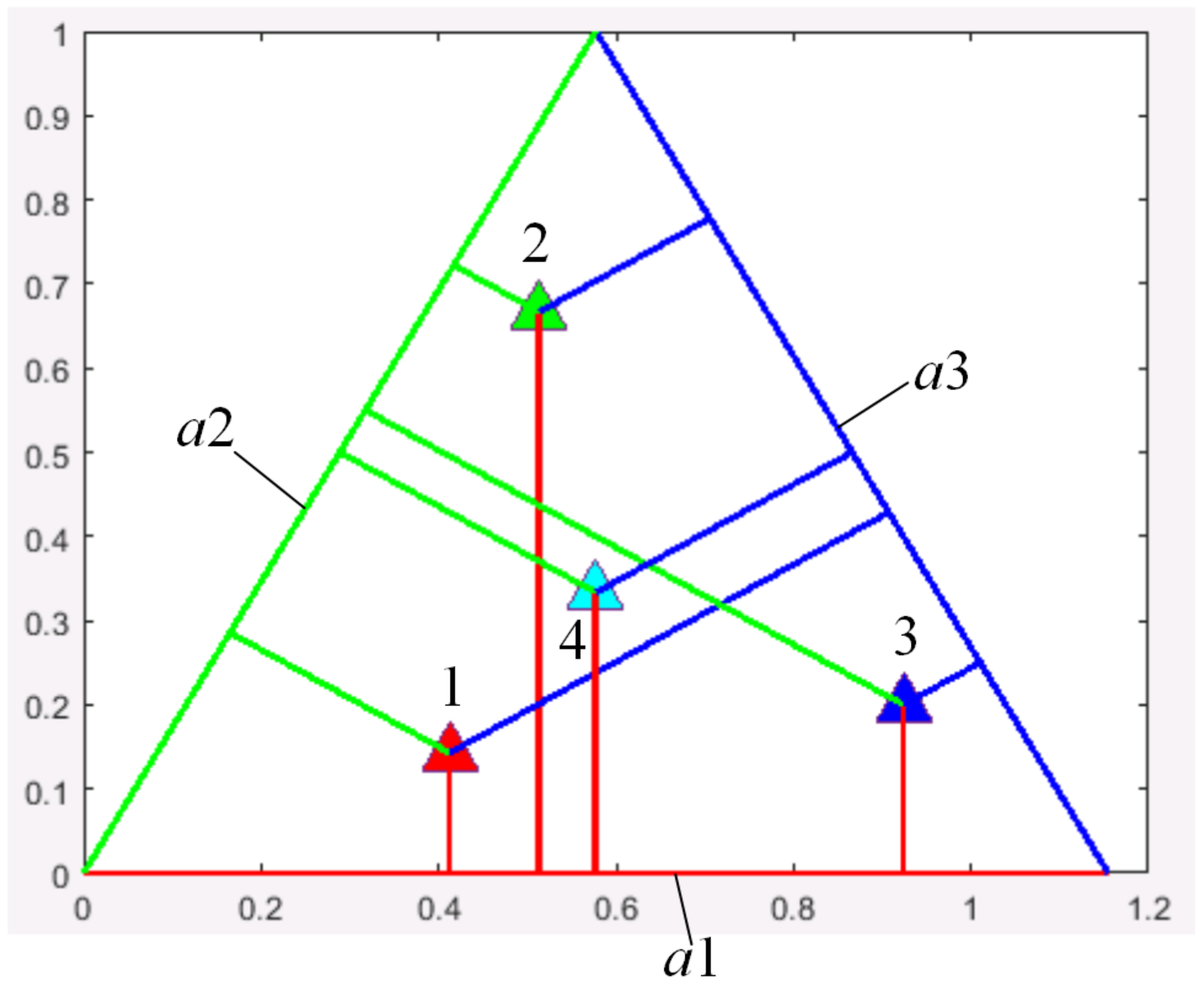
In this Appendix A, we give the mathematical basis of a cognitive graphic tool 2-simplex. This object is known from Discrete Mathematics and represents an equilateral triangle. Within the 2-simplex, we can render any three values a, b, and c simultaneously. In this sense the tool serves for dimensionality reduction, making the visual information (graphs, points, curves, waveforms, etc.) more comprehensible to a human being.
Theorem A1.
Suppose is a set of simultaneously non-zero numbers in a 2-simplex. Then, there is one and only one point in which the following condition is correct, where is the distance from the point to the i-th side, and n is the dimension of the regular simplex. In our case, .
Factors represent the degrees of proximity of an object , which is characterized by the three given numbers, to each side of the 2-simplex. In geometrical interpretation are the perpendiculars connecting the point and the three sides of the graphic tool under study.
Thus, in 2-simplex, the sum of distances . Mathematical description of the 2-simplex can be written as a system of equations:
where is a scaling factor such that . In our case, and represents the height of the triangle.
This theorem was used in more than 30 applied intelligent systems to create three instrumental tools capable of revealing different kinds of regularities for making diagnostic, classification, organizational, and control decisions.
A more detailed mathematical basis of 2-simplex is outlined in a thesis [27].
The software below represents one possible realization of the 2-simplex for rendering some values.
An illustrative example of implementing a cognitive graphic tool 2-simplex is shown in Figure A1.
Table A1.
Data table for 2-simplex.
Table A1.
Data table for 2-simplex.
| Point No | Value a1 | Value a2 | Value a3 |
|---|---|---|---|
| 1 | 0.2 | 0.4 | 0.8 |
| 2 | 0.6 | 0.2 | 0.1 |
| 3 | 0.2 | 0.7 | 0.1 |
| 4 | 0.5 | 0.5 | 0.5 |

Figure A1.
Rendering four values in 2-simplex.
Figure A1.
Rendering four values in 2-simplex.
| Listing A1. 2-simplex in MATLAB. |
|
%data values %a1=0.2;a2=0.4;a3=0.8; %a1=0.6;a2=0.1;a3=0.2; %a1=0.2;a2=0.7;a3=0.1; a1=0.5;a2=0.5;a3=0.5; %scaling factor alpha=1/(a1+a2+a3); %heights h1=alpha*a1; h2=alpha*a2; h3=alpha*a3; %plot a triangle X1=[0 2/sqrt(3)]; Y1=[0 0]; plot(X1,Y1,’r’,’LineWidth’,2); hold on; X2=[2/sqrt(3) 1/sqrt(3)]; Y2=[0 1]; plot(X2,Y2,’b’,’LineWidth’,2); hold on; X3=[1/sqrt(3) 0]; Y3=[1 0]; plot(X3,Y3,’g’,’LineWidth’,2); hold on; %basis vectors P1 = [1/sqrt(3) 1]; P2 = [2/sqrt(3) 0]; %vectors to calculate of coordinates of a point V1=h1*P1; V2=h2*P2; %plotting the point in 2-simplex plot(V1(1)+V2(1),V1(2)+V2(2),’’,’MarkerSize’,15,’MarkerFaceColor’,[0, 1, 1]); %plotting the perpendiculars proportional to the values Xa1=[V1(1)+V2(1) V1(1)+V2(1)]; Ya1=[V1(2) 0]; plot(Xa1,Ya1,’r’,’LineWidth’,2); Xa2=[V1(1)+V2(1) V1(1)+V2(1)*cos(pi/3)2]; Ya2=[V1(2) V1(2)+V2(1)*cos(pi/3)*sin(pi/3)]; plot(Xa2,Ya2,’g’,’LineWidth’,2); Xa3=[V1(1)+V2(1) V1(1)+V2(1)+h3*sin(pi/3)]; Ya3=[V1(2) V1(2)+V2(2)+h3*cos(pi/3)]; plot(Xa3,Ya3,’b’,’LineWidth’,2); |
Appendix B
| Listing A2. Logical Block in MATLAB. |
| function [D1, D2] = fcn(u) if (u<0.5 & u>0) D1 = 0; D2=(u/0.5); elseif (u>=0.5 & u<=1) D1 = (u/0.5) - 1; D2=1; elseif u<0 D1=0; D2=0; else D1=1; D2=1; end [D1, D2]; |
References
- Krauter, S.C.W. Solar Electric Power Generation, 13th ed.; Springer: Berlin/Heidelberg, Germany, 2006; pp. 1–18. [Google Scholar]
- Matthiss, B.; Momenifarahani, A.; Binder, J. Storage Placement and Sizing in a Distribution Grid with High PV Generation. Energies 2021, 14, 303. [Google Scholar] [CrossRef]
- Grabara, J.; Tleppayev, A.; Dabylova, M.; Mihardjo, L.W.W.; Dacko-Pikiewicz, Z. Empirical Research on the Relationship amongst Renewable Energy Consumption, Economic Growth and Foreign Direct Investment in Kazakhstan and Uzbekistan. Energies 2021, 14, 332. [Google Scholar] [CrossRef]
- Amato, A.; Bilardo, M.; Fabrizio, E.; Serra, V.; Spertino, F. Energy Evaluation of a PV-Based Test Facility for Assessing Future Self-Sufficient Buildings. Energies 2021, 14, 329. [Google Scholar] [CrossRef]
- Swaminathan, G.; Ramesh, V.; Umashankar, S.; Sanjeevikumar, P. Investigations of Microgrid Stability and Optimum Power Sharing Using Robust Control of Grid Tie PV Inverter. In Advances in Smart Grid and Renewable Energy; SenGupta, S., Zobaa, A.F., Sherpa, K.S., Bhoi, A.K., Eds.; Springer: Singapore, 2018; pp. 379–387. [Google Scholar]
- Abdullah, M.F.; Ahmed, M.; Hasan, K.N.M. Feasibility Study on Hybrid Renewable Energy to Supply Unmanned Offshore Platform. In Sustainable Electrical Power Resources through Energy Optimization and Future Engineering; Sulaiman, S.A., Kannan, R., Karim, S.A.A., Nor, N.M., Eds.; Springer: Singapore, 2018; pp. 65–85. [Google Scholar]
- Elmouatamid, A.; Ouladsine, R.; Bakhouya, M.; El Kamoun, N.; Khaidar, M.; Zine-Dine, K. Review of Control and Energy Management Approaches in Micro-Grid Systems. Energies 2021, 14, 168. [Google Scholar] [CrossRef]
- Haq, S.; Biswas, S.P.; Hosain, M.K.; Rahman, M.A.; Islam, M.R.; Jahan, S. A Modular Multilevel Converter with an Advanced PWM Control Technique for Grid-Tied Photovoltaic System. Energies 2021, 14, 331. [Google Scholar] [CrossRef]
- Photovoltaic/Solar Array Simulation Solution. Available online: https://www.keysight.com/ru/ru/assets/3120-1365/data-sheets/Photovoltaic-Solar-Array-Simulation-Solution.pdf (accessed on 21 February 2022).
- E4360 Series Modular Solar Array Simulators. Available online: https://www.keysight.com/ru/ru/products/dc-power-supplies/dc-power-solutions/e4360-series-modular-solar-array-simulators.html (accessed on 21 February 2022).
- Chen, Y.; Vinco, S.; Pagliari, D.J.; Montuschi, P.; Macii, E.; Poncino, M. Modeling and Simulation of Cyber-Physical Electrical Energy with SystemC-AMS. IEEE Trans. Sustain. Comput. 2020, 5, 552–567. [Google Scholar] [CrossRef]
- Canadian Solar CS6K-270P (270W) Solar Panel. Available online: http://www.solardesigntool.com/components/module-panel-solar/Canadian-Solar/3514/CS6K-270P/specification-data-sheet.html (accessed on 18 February 2022).
- Tao, Z.; Qunjing, V. Application of MATLAB/SIMULINK and PSPICE simulation in teaching power electronics and electric drive system. In Proceedings of the Eighth International Conference on Electrical Machines and Systems (ICEMS-2005), Nanjing, China, 27–29 September 2015. [Google Scholar]
- Villalva, M.G.; Gazoli, J.R.; Filho, E.R. Comprehensive Approach to Modeling and Simulation of Photovoltaic Arrays. IEEE Trans. Power Electron. 2009, 24, 1198–1208. [Google Scholar] [CrossRef]
- Cubas, J.; Pindado, S.; de Manuel, C. Explicit Expressions for Solar Panel Equivalent Circuit Parameters Based on Analytical Formulation and the Lambert W-Function. Energies 2014, 7, 4098–4115. [Google Scholar] [CrossRef] [Green Version]
- Obukhov, S.; Plotnikov, I.; Kryuchkova, M. Simulation of Electrical Characteristics of a Solar Panel. IOP Conf. Ser. Mater. Sci. Eng. 2016, 132, 0112017. [Google Scholar] [CrossRef] [Green Version]
- Gow, J.A.; Manning, C.D. Development of a Photovoltaic Array Model for Use in Power-Electronics Simulation Studies. IEEE Proc. Electr. Power Appl. 1999, 146, 193–200. [Google Scholar] [CrossRef]
- Zekry, A.; Shaker, A.; Salem, M. Solar Cells and Arrays: Principles, Analysis, and Design. In Advances in Renewable Energies and Power Technologies; Yahyaoui, I., Ed.; Elsevier: Amsterdam, The Netherlands, 2018; pp. 3–56. [Google Scholar]
- Vinco, S.; Chen, Y.; Macli, E.; Poncino, M. A Diode-Aware Model of PV Modules from Datasheet Specifications. In Proceedings of the 2020 Design, Automation and Test in Europe Conference and Exhibition (DATE), Grenoble, France, 9–13 March 2020. [Google Scholar]
- Rashid, M. Power Electronics Handbook, 4th ed.; Butterworth-Heinemann, Elsevier: Oxford, UK, 2018. [Google Scholar]
- Yudintsev, A.; Tkachenko, A.; Lyapunov, D. Adjusting the Current Controller for a Load Simulator Based on the Boost DC-DC Converter. In Proceedings of the 15th International Siberian Conference on Control and Communications, SIBCON, Kazan, Russia, 13–15 May 2021. [Google Scholar]
- Pravikova, A.; Lyapunov, D.; Yudintsev, A. Controller adjustment using symmetrical optimum for load simulator based on boost converter. In Proceedings of the International Conference on Electrical, Computer, Communications and Mechatronics Engineering, ICECCME, Reduit, Mauritius, 7–8 October 2021. [Google Scholar]
- Astrom, K.J.; Hagglund, T. PID Controllers: Theory, Design, and Tuning, 2nd ed.; Research Triangle Park: Raleigh, NC, USA, 1995. [Google Scholar]
- Bruce, P.; Bruce, A. Practical Statistics for Data Scientists; O’Reilly Media, Inc.: Sebastopol, CA, USA, 2016. [Google Scholar]
- How to Paint a Small Non-Overlapping Area. Available online: https://www.stackfinder.ru/questions/66339665/in-matlab-how-to-shade-a-small-non-overlapping-area-when-two-plots-and-a-thresh (accessed on 19 February 2022).
- Yankovskaya, A.E.; Yamshanov, A.V. Family of 2-simplex cognitive tools and their application for decision-making and its justifications. arXiv 2016, arXiv:1601.01497. [Google Scholar]
- Yamshanov, A.V. Models and Methods of Parallel Computing for Designing Fail-Safe Diagnostic Tests in Intelligent Systems with Cognitive Component. Ph.D. Thesis, Tomsk State University of Control Systems and Radioelectronics, Tomsk, Russia, 2017. [Google Scholar]
- Zhusubaliyev, Z.T.; Mosekilde, E. Bifurcations and Chaos in Piecewise-Smooth Dynamical Systems; World Scientific: Singapore, 2003; pp. 231–277. [Google Scholar]
- Dorf, R.; Bishop, R. Modern Control Theory, 13th ed.; Pearson Education: Hoboken, NJ, USA, 2017; pp. 160–163. [Google Scholar]
- Shrud, M.A.; Kharaz, A.; Ashur, A.S.; Shater, M.; Benyoussef, I. A Study of Modeling and Simulation for Interleaved Buck Converter. In Proceedings of the 2010 1st Power Electronic & Drive Systems & Technologies Conference (PEDSTC), Tehran, Iran, 17–18 February 2010; pp. 28–35. [Google Scholar]


Publisher’s Note: MDPI stays neutral with regard to jurisdictional claims in published maps and institutional affiliations. |
© 2022 by the authors. Licensee MDPI, Basel, Switzerland. This article is an open access article distributed under the terms and conditions of the Creative Commons Attribution (CC BY) license (https://creativecommons.org/licenses/by/4.0/).