Abstract
In recent years, big data and artificial intelligence technology have developed rapidly and are now widely used in fields of geophysics, well logging, and well test analysis in the exploration and development of oil and gas. The development of shale gas requires a large number of production wells, so big data and artificial intelligence technology have inherent advantages for evaluating the productivity of gas wells and analyzing the influencing factors for a whole development block. To this end, this paper combines the BP neural network algorithm with random probability analysis to establish a big data method for analyzing the influencing factors on the productivity of shale gas wells, using artificial intelligence and in-depth extraction of relevant information to reduce the unstable results from single-factor statistical analysis and the BP neural network. We have modeled and analyzed our model with a large amount of data. Under standard well conditions, the influences of geological and engineering factors on the productivity of a gas well can be converted to the same scale for comparison. This can more intuitively and quantitatively reflect the influences of different factors on gas well productivity. Taking 100 production wells in the Changning shale gas block as a case, random BP neural network analysis shows that maximum EUR can be obtained when a horizontal shale gas well has a fracture coefficient of 1.6, Type I reservoir of 18 m thick, optimal horizontal section of 1600 m long, and 20 fractured sections.
1. Introduction
After more than ten years of exploration and development, shale gas resources have been effectively exploited in China [1]. With deepening development, more than 2000 shale gas wells have been constructed, and the scale of production data is increasing in China [2,3]. Determining how to analyze the factors influencing the productivity of gas wells is important for the development and optimization of production blocks. In recent years, the application of big data and artificial intelligence in oil and gas fields has accelerated and become a powerful driving force of the technological revolution in the petroleum industry. Deng et al. (2000) took the peak value of the derivative curve and the position of the horizontal line of the radial stream as the inputs of a three-layer feedforward neural network to estimate well test parameters [4]. In 2011, Asadisaghandi et al. used a neural network to predict the PVT relationship of oil products [5], and Memon predicted bottom-hole flowing pressure based on neural network models [6]. Zhang used a recurrent neural network to study the generation and repair of synthetic well logs [7]. Li proposed an automatic well test interpretation method for radial composite reservoirs based on a convolutional neural network [8]. Big data and artificial intelligence technology have been widely used in many fields, such as the evaluation of shale reservoir [9,10,11,12], productivity analysis [13,14,15,16], and engineering technology [17,18,19]. Based on these technologies, the impact of different practical factors on energy production can be fully exploited to lay the foundation for the next evaluation and extraction work.
According to the published literature, for evaluating shale gas exploration and development in China, artificial intelligence methods are mainly used in the fields of geophysics [20,21,22], well logging [23,24,25], and well test analysis [26,27,28,29]. Productivity evaluation and analysis of influencing factors on shale gas wells in an entire development block are weak. The productivity of a shale gas well is affected by many factors, such as geology and engineering. The results of conventional statistical methods are not very regular; thus, effective analysis cannot be realized. In particular, the shale gas industry has entered a rapid and large-scale development stage. As the production scale expands, to achieve efficient development, some urgent problems should be solved, such as the relationship between geological engineering parameters and gas well productivity, and discovering optimal parameters for gas well production based on the analysis of geological characteristics and engineering parameters in many blocks.
Recently, with the development of deep learning, many machine learning and deep learning methods have been used in gas well productivity. Huang et al. used a genetic algorithm to optimize the kernel function type, kernel function parameters, and error penalty factor of their model and established a GA-SVM model [30]. Li et al. developed a deep learning approach based on a long short-term memory (LSTM) neural network model to predict well performance considering manual operations [31]. Shi et al. proposed a novel combined long short-term memory (LSTM) and multilayer perceptron (MLP) neural network to efficiently predict geothermal productivity considering constraints [32]. However, these methods do not take into account the effects of random noise on the model in practical applications, while failing to effectively model the potential relationships between different input features.
To solve the above problems, based on the development characteristics of shale gas wells in typical shale gas blocks, we take advantage of big data and artificial intelligence to analyze the influences of different parameters on gas well productivity.
Our main contributions are summarized as follows:
- (1)
- We are the first to analyze the impact of different address characteristics and engineering parameters on gas well capacity by taking advantage of big data and artificial intelligence.
- (2)
- To better analyze the effect of different parameters on gas well capacity, we designed a random BP neural network analysis method, which can effectively learn the effect of different parameters on capacity.
- (3)
- With extensive experiments on real data, our method can effectively and intuitively reflect the influence of different factors on capacity and calculate the optimal parameters.
2. Materials and Methods
2.1. Limitations of Conventional Methods
2.1.1. Statistical Method
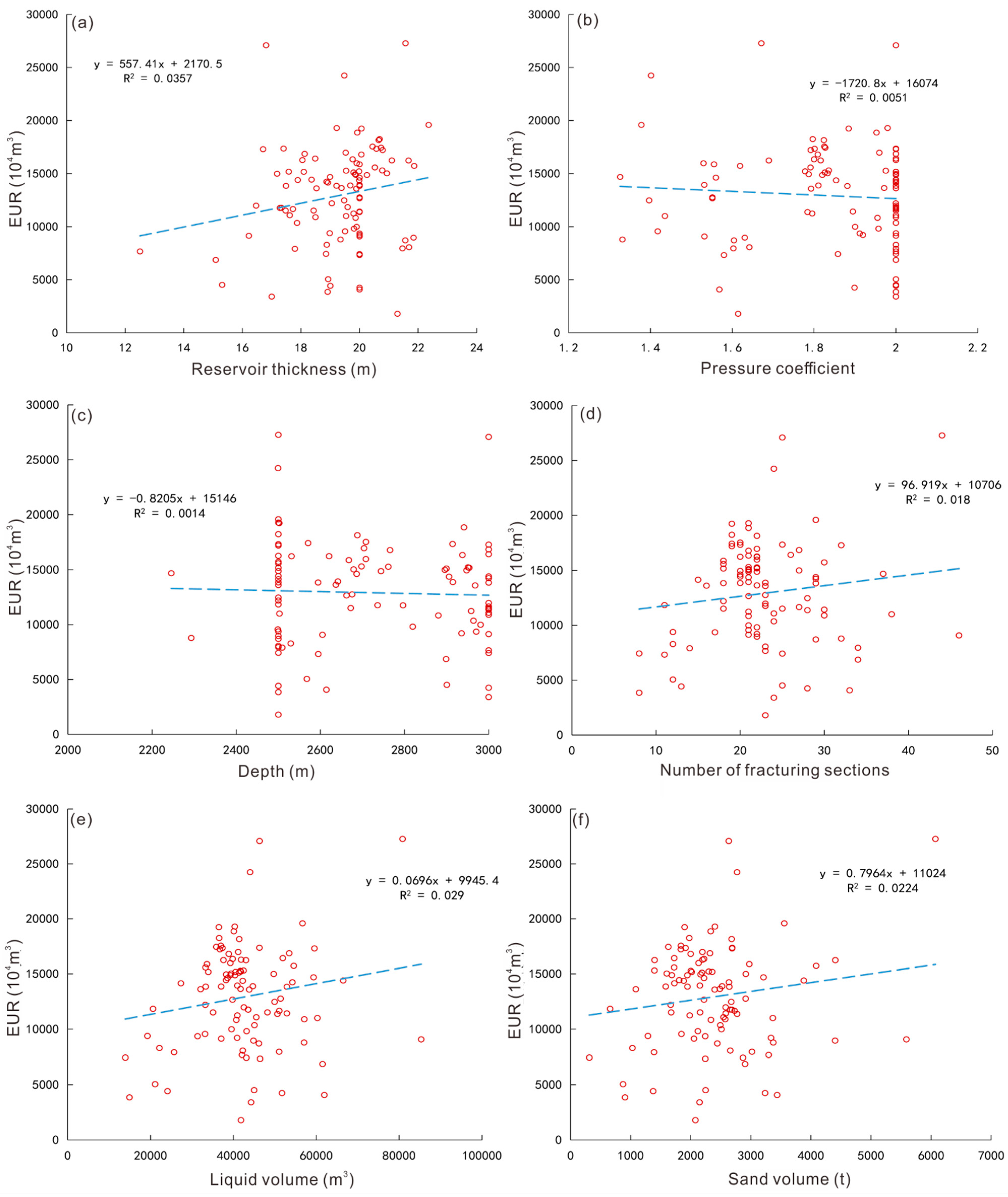
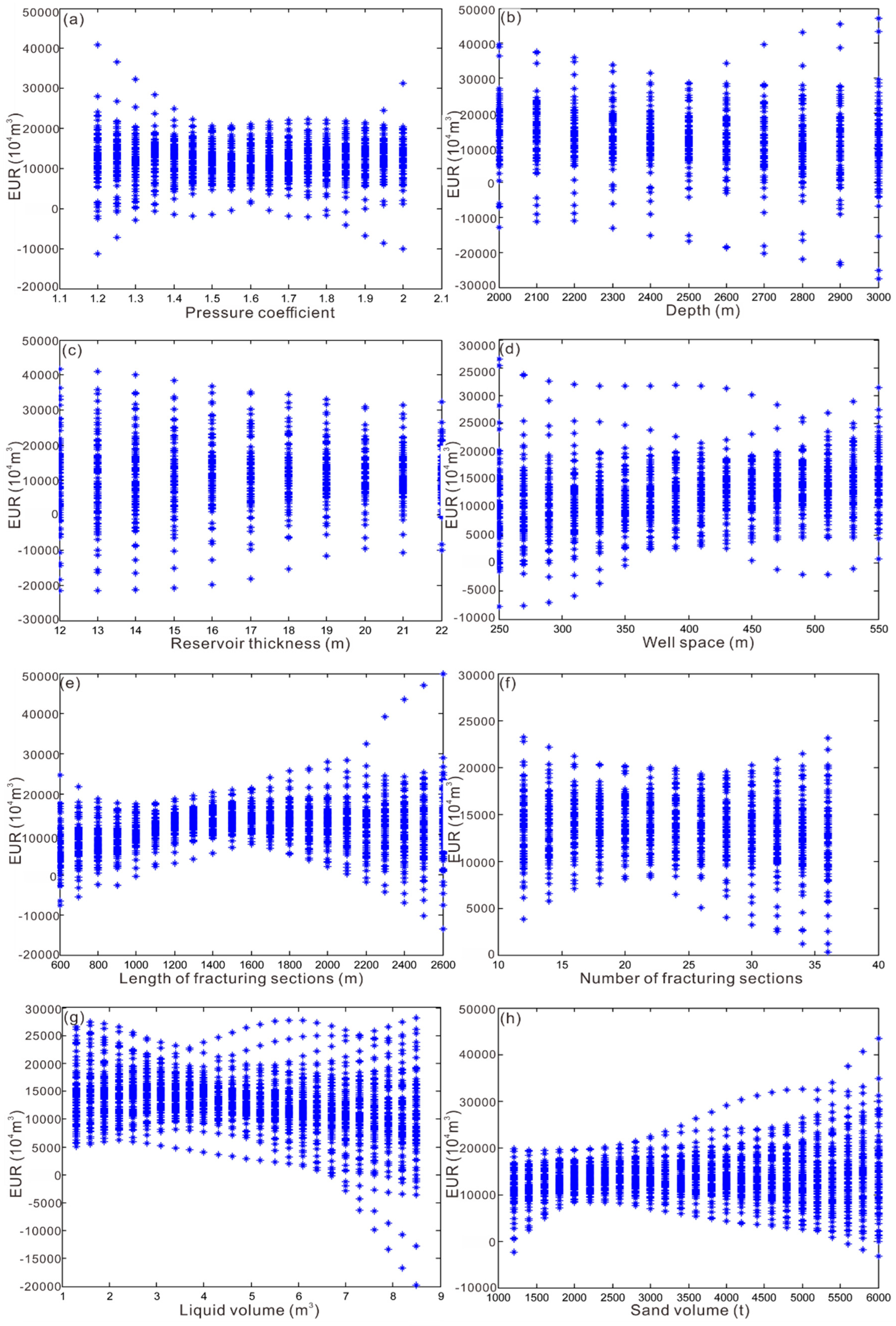
Due to the differences in geological and engineering conditions of shale gas wells, the statistical method is used for single-factor analysis. However, due to interference among parameters, the statistical data are scattered and the relationships are not obvious. This paper takes 100 horizontal shale gas wells, which have been producing for more than 1 year in the Changning block as a case and adopts the Duong method to fit the gas production curve [29] to obtain the 20-year EUR (estimated ultimate recovery) of the gas wells. The statistical relationship between the parameters and EUR shows that the data in each graph are scattered. The parameters include the thickness of the Type I reservoir, pressure coefficient, burial depth, number of fracturing sections, sand volume, and liquid volume, etc. Although there is some relationship between the parameters and EUR, the statistical correlation coefficient is only 0.0051–0.0357, and the correlation is not obvious (Figure 1).
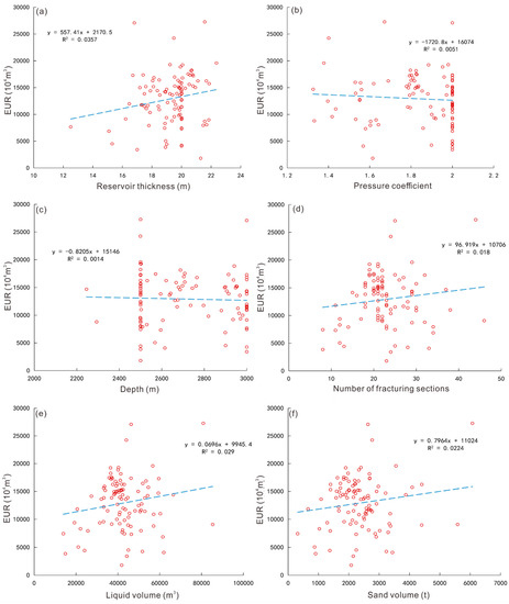
Figure 1.
Statistical relationships between parameters and EUR of a well in the production block. (a) Relationship between EUR and reservoir thickness; (b) relationship between EUR and pressure coefficient; (c) relationship between EUR and depth; (d) relationship between EUR and number of fracturing sections; (e) relationship between EUR and liquid volume; (f) relationship between EUR and sand volume.
2.1.2. BP Neural Network Analysis
The BP neural network model is one of the most widely used neural network models proposed by Rumelhart and McCelland. It is characterized by a network model that is trained and learns according to an error backpropagation algorithm. This method includes two processes.
First, information is forward propagated in computer hardware, and large calculation workload is no longer a problem. However, network stability still exists due to the different quantities of machine learning samples for specific cases.
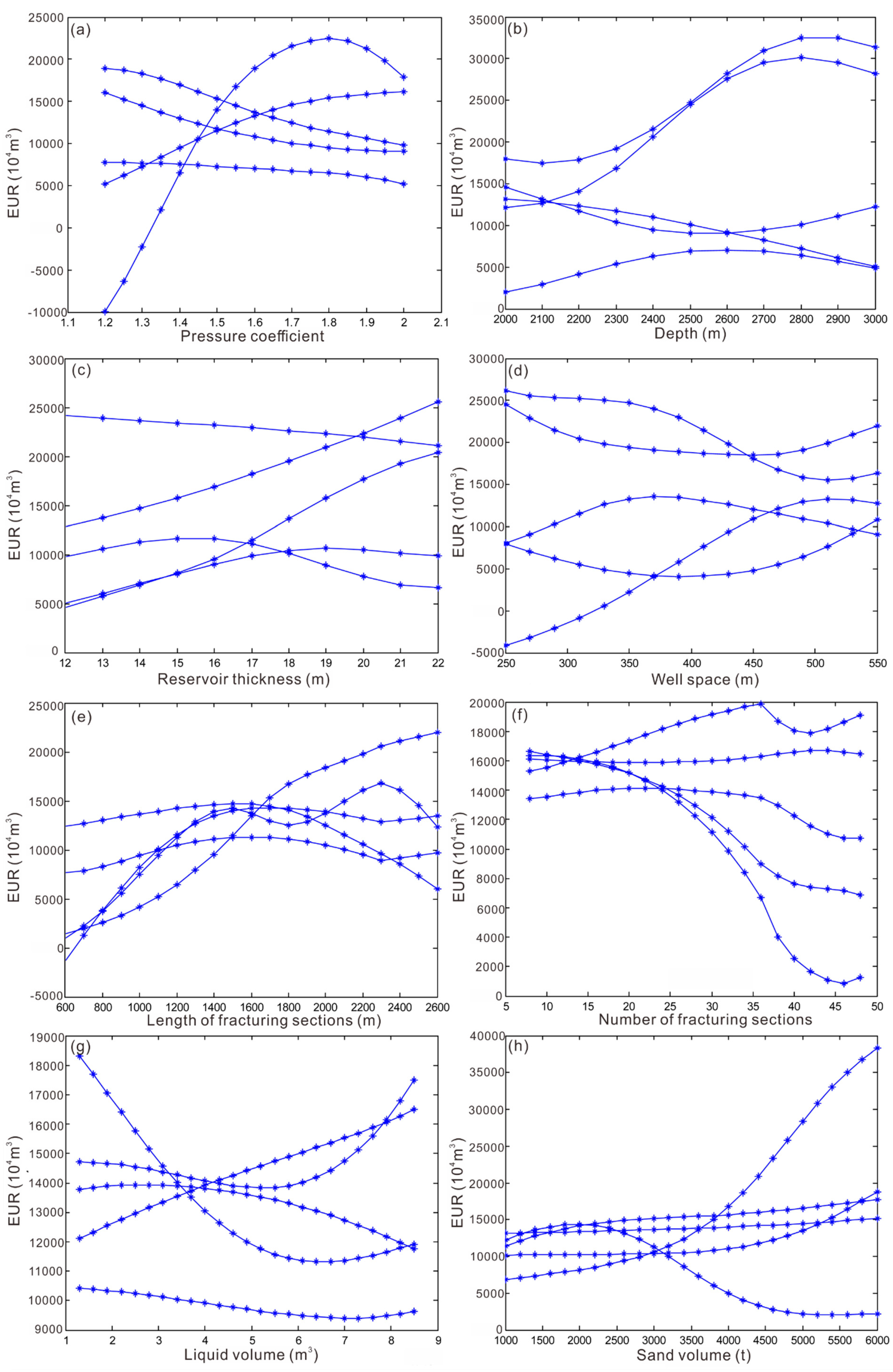
Taking 100 shale gas wells with a long production history in the Changning block as a case, we input five different combinations of the same samples to analyze the relationship between the parameters and the EUR. The parameters include the thickness of Type I reservoirs, pressure coefficient, burial depth, number of fracturing sections, sand volume, and liquid volume, etc. The analysis results show that the influence of each factor on EUR is quite different, and the analysis results of different combinations are quite different (Figure 2).
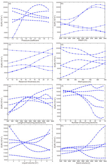
Figure 2.
BP neural network analysis of 5 different combinations of the same samples. (a) Relationships between predicted EUR and pressure coefficient; (b) relationship between EUR and depth; (c) relationship between EUR and reservoir thickness; (d) relationship between EUR and number of fracturing sections; (e) relationship between EUR and liquid volume; (f) relationship between EUR and sand volume; (g) relationship between EUR and liquid volume; (h) relationship between EUR and sand volume.
2.2. Random BP Neural Network Analysis
2.2.1. Basic Ideas
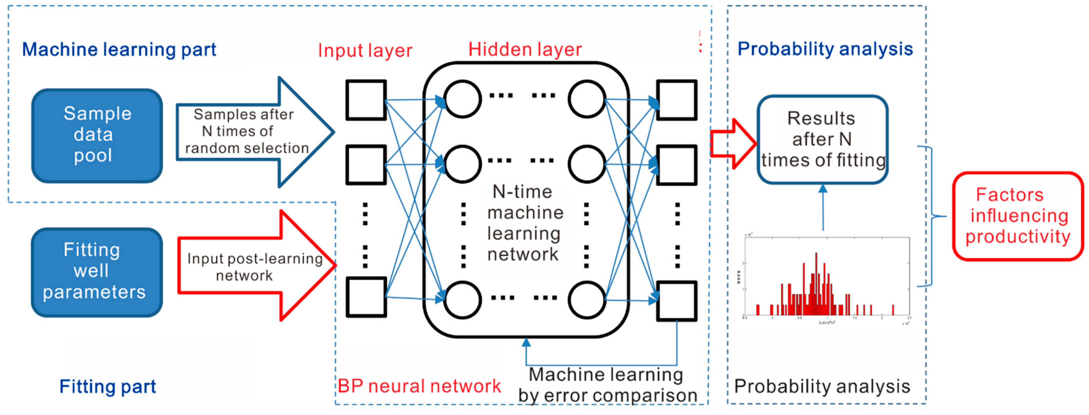
We combined random probability analysis with a BP neural network to solve the problem in three steps. First, we solved the problem of different results from different sample combinations and different input orders by generalizing the input parameters of the samples through multiple random sampling. Second, we input the multiple randomly selected sample sets into the BP neural network and established multiple post-learning network models to realize the generalization of the simulation process of the BP neural network and improve the stability of the model. Third, we established a set of parameters for the fitted well by changing the parameters to analyze the sensitivity of specific parameters of productivity under uniform parameter conditions (Figure 3). In the training process, we used random sampling to analyze and model the big data. Thanks to the big data support, our method has a high level of correctness and robustness in practical applications.

Figure 3.
Schematic diagram of random BP neural network analysis method.
2.2.2. Analysis Method
In the specific calculation process, the random BP neural network analysis method mainly includes two parts: random BP network modeling and data prediction analysis.
Random BP Network Modeling
(1) Establishing the input sample sets IRandum. We selected N samples to form the sample data pool A, with each sample in A a vector composed of samples which contain k feature parameters p. We randomly selected n samples, n ≤ N, as the input Bi sample set for neural network learning. Then, after repeating the above process M times, we obtained M neural network learning input sample sets IRandum. The details are as follows:
a = [p1, p2,..., pK]
A = {a1, a2,..., aN}
O = {o1, o2,..., oN}
We randomly took n samples in the sample pool A to form a new sample set Yi, and repeated random sampling multiple times to form M input sample sets InRandum, where n ≤ N.
Bi = {ai1, ai2,..., ain}
The output results corresponding to the selected sample are as follows:
Oi = {oi1, oi2,..., oin}
IRandum = {B1, B2,..., BM}
(2) Establishing the BP network collection NetRandum. We input each new sample set Yi, which is randomly selected in the sample data pool A, into the BP neural network and formed the learned network model Neti through continuous recurrent comparison and machine learning with Oi. We input the sample sets of M random selection into the BP neural network, respectively, and formed the BP neural network set NetRandum, composed of post-learning M network models.
Neti = F(Bi,Oi)
{Net1, Net2,..., NetM}
Data Prediction Analysis
(1) Data fitting. The vector Xi composed of K parameters was input into the BP network set NetRandum, and after the operation by M network models, M prediction results yi were obtained. The M prediction results formed the set Yi. Under the same conditions of the other parameters, the value of a parameter vector in X was changed in an orderly manner (f times) to form the prediction data set Input and the corresponding output prediction result set Output so as to analyze the sensitivity of the parameter change to the prediction result.
Xi = [xi1, xi2,..., xiK]
Yi = {yi1, yi2,..., yiM}
Yi = F(Xi, Neti)
Input = {X1, X2,..., Xf}
Output = {Y1, Y2,..., Yf}
(2) Probability analysis. Because each Yi in the prediction result set Output is a prediction result composed of M data, probability and statistical methods were used to analyze its statistical laws, which generally conforms to the normal distribution. Then, we obtained the expected probability ei of Yi and the data width of a specific confidence curve.
3. Results and Discussion
3.1. Network Modeling with Big Data
Taking the Changning block as a case, we selected the data of 100 production wells with a production history of more than 1 year as the sample data pool. The input vector of each sample includes eight parameters: pressure coefficient, buried depth, the thickness of Type I reservoir, well spacing, length of fracturing horizontal section, number of fracturing sections, fluid volume, and sand volume. The output results are the 20-year estimated ultimate recovery (EUR) obtained by the Duong method. We randomly selected 80 samples as a new sample set each time and repeated this 100 times, forming 100 randomly selected new sample sets. The 100 new sample sets were input into a BP neural network model with 10 hidden layers, and the random BP neural network model was completed after machine learning.
3.2. Analysis of Factors Affecting Well Productivity
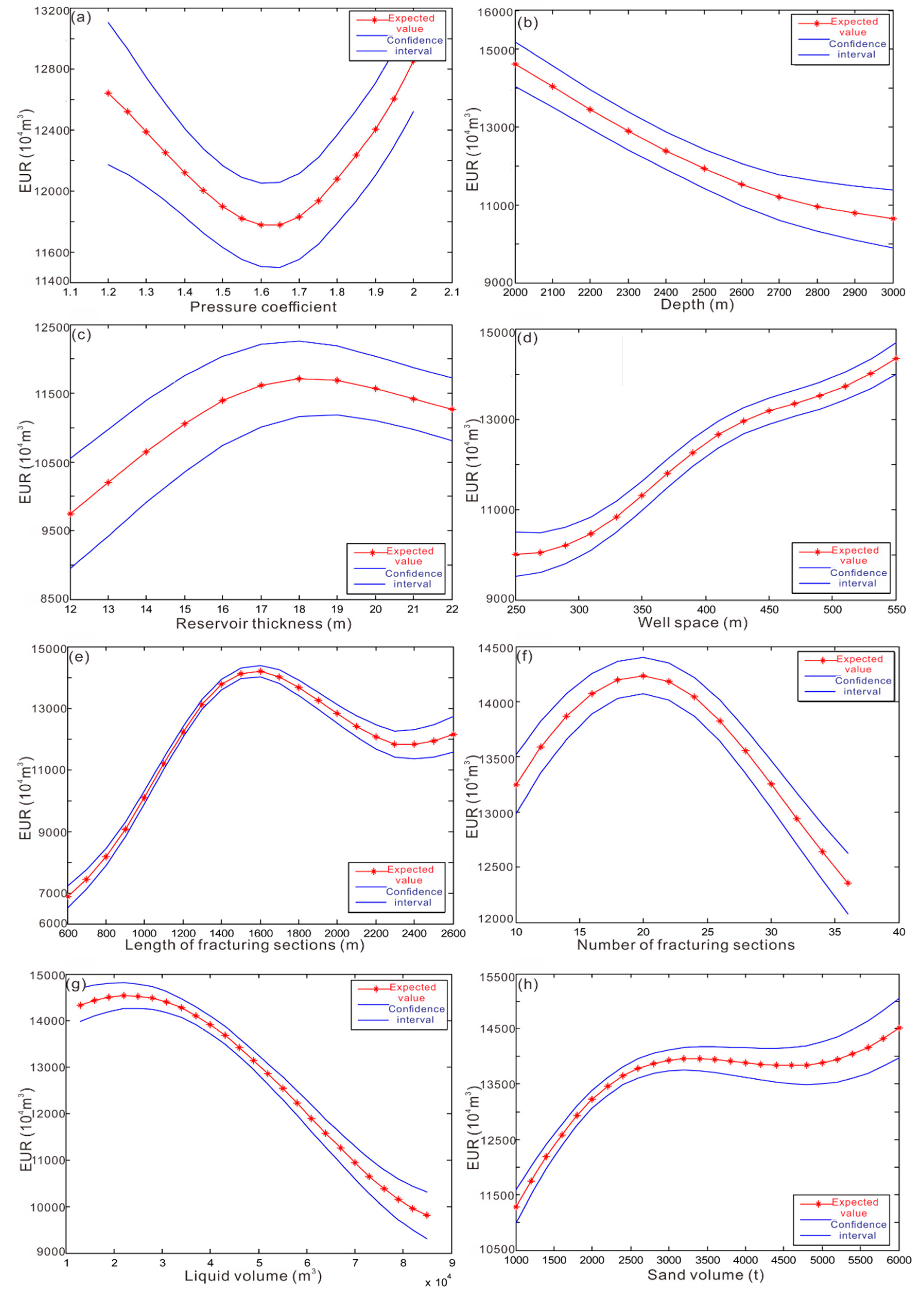
In order to analyze the influence of different parameters on the 20-year EUR of a gas well under the same conditions, we set a standard well with reservoir pressure coefficient of 1.8, buried depth of 2700 m, the thickness of Type I reservoir of 19 m, well spacing of 400 m, horizontal section length of 1400 m, number of fracturing sections of 33, liquid volume of 42,000 m3, and sand volume of 2300 tons. On the basis of a random BP neural network constructed with samples of 100 production wells in the Changning block, we established a predictive input data set, Input, by changing one of the parameters. The output result after input into the network is shown in Figure 4, that is, the 20-year EUR of the gas well under different parameter values. Then, we performed a probability analysis of the input results to obtain the probability expectation value and the interval of 50% confidence coefficient (Figure 5). Taking the 20-year EUR as the optimization goal, the fracturing coefficient of the horizontal well for the development of the shale gas in the Changning block is 1.6, and the single-well EUR shows a downward trend as the buried depth increases, which is consistent with the great difficulty of engineering technology with the increase in burial depth. The single-well EUR generally changed little after the thickness of the Type I reservoir exceeded 18 m, indicating that the vertical spread of induced fractures in a horizontal well was limited. The lateral well spacing and the EUR change are generally positively correlated in this study. The optimal length of the horizontal section of a horizontal well is 1600 m, and the optimal number of fracturing sections is 20, which are consistent with the result that the increase in the horizontal section length and the number of fracturing sections will increase the fracturing difficulty and result in an unsatisfactory fracturing effect.
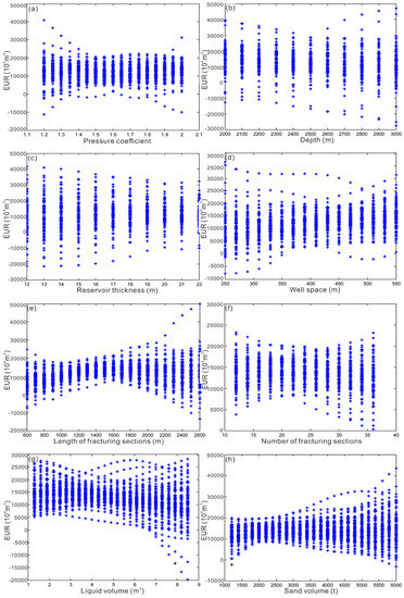
Figure 4.
Fitted results of 200 times of random BP neural network for a standard well in Changning block. (a) Relationship between EUR and pressure coefficient; (b) relationship between EUR and depth; (c) relationship between EUR and reservoir thickness; (d) Relationship between EUR and number of well space; (e) relationship between EUR and length of fracturing sections; (f) relationship between EUR and number of fracturing sections; (g) relationship between EUR and liquid volume; (h) relationship between EUR and sand volume.
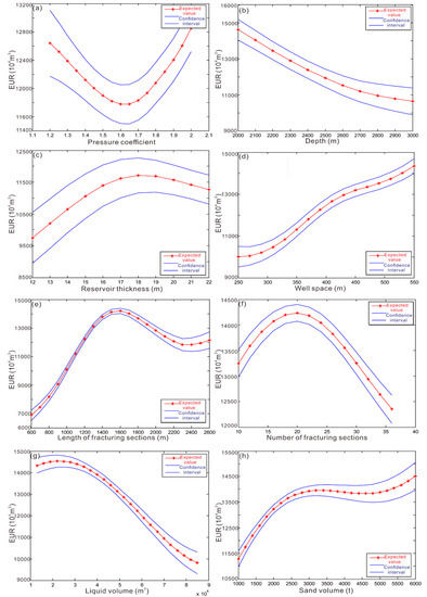
Figure 5.
Fitted expected value and interval of 50% confidence coefficient on random BP neural network for a standard well in Changning block. (a) Relationship between EUR and pressure coefficient; (b) relationship between EUR and depth; (c) relationship between EUR and reservoir thickness; (d) relationship between EUR and number of well space; (e) relationship between EUR and length of fracturing sections; (f) relationship between EUR and number of fracturing sections; (g) relationship between EUR and liquid volume; (h) relationship between EUR and sand volume.
The ablation experiments with different parameters revealed (shown in Figure 5) that the pressure coefficient, reservoir thickness, length of fracturing sections, and number of fracturing sections are nonlinearly related to EUR, so in practice, the parameters need to be selected according to the discriminatory situation of the model. Meanwhile, using Figure 5, we can find that the length of fracturing sections has the greatest effect on EUR.
Table 1 and Figure 6 show the results of capacity prediction by our method compared with the ground truth, and the comparison shows that our method can predict the capacity effectively. However, the results are not satisfactory on the prediction of well 16, which we believe is due to some error in the actual data measurement, and if the error is ignored, better results will be obtained.

Table 1.
The Results of Horizontal Shale Gas Well Capacity Prediction.
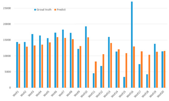
Figure 6.
Horizontal Shale Gas Well Capacity Prediction vs. Ground Truth.
We selected the following models for comparison, including machine learning models: Logistic Regression (LR) [33] and Support Vector Regression (SVR) [34], and deep learning models: Long Short-Term Memory (LSTM) [35] and Convolutional Neural Networks (CNN) [36]. In order to verify the superiority of the models, Mean Absolute Error (MAE) was used as the evaluation metric, and the results are shown in Table 2.
Table 2.
Comparison of our model with other models in terms of MAE; lower MAE values indicate better results.
By comparison, we find that our model can achieve optimal results. We believe this is for the following reasons: (1) the traditional machine learning model has a small number of parameters and cannot learn the implicit relationship between different variables well. (2) LSTM is more suitable for temporal tasks, whereas CNN works better for image-like tasks, but it is not as good as the BP neural network for learning the implicit relationship between different variables. (3) Our random BP approach can effectively increase the robustness of the model, making it applicable to different data features.
3.3. Advantages of the Method Proposed in the Paper
(1) Conventional statistical analysis is interfered with by multiple factors and conceals the internal information of the data, particularly the correlation between a single factor, and the EUR of the gas well is poor. The method proposed in the paper analyzes the influence of each parameter under multi-scale conditions. We obtained the maximum expected value of EUR and an interval of 50% confidence coefficient through random probability generalization processing, which better shows the influence of a factor on EUR.
(2) It removes human interference in data analysis and has good fault tolerance for data. The errors of individual data are effectively suppressed by machine learning from the neural network model established by big data and reducing the weight of the fault value in the network. Eventually, the analysis result will fall within the high probability interval of normal distribution.
4. Conclusions
By combining a BP neural network algorithm with random probability analysis, we established a productivity analysis method for analyzing the influencing factors on the productivity of shale gas wells based on random BP neural network. This method can make full use of effective information through artificial intelligence learning from big data and solve problems such as unstable results from single-factor statistical methods and BP neural network methods. For a standard well, the influence of every geological/engineering factor on the well productivity can be converted to the same scale for comparison. The results can more intuitively and quantitatively reflect the influences of different geological and engineering factors on gas well productivity. Through extensive experimental analysis, this model outperforms other machine learning models and deep learning models and has a higher degree of robustness.
5. Parameter Description
A is the sample data pool composed of all N samples;
B is the new sample set composed of n samples randomly selected from A;
Bi is the ith sample;
Input is the predictive input data set composed of f Xi;
InRandum is the set of new samples B after randomly selecting M times;
K is the number of parameters in a;
M is the times of random selection;
N is the number of samples in the sample data pool A;
Net is the post-learning BP neural network model;
Neti is the model established for the i-th time;
NetRandum is the neural network set established after M times of machine learning;
O is the set composed of n output results o;
Oi is the set of output results corresponding to Bi;
Output is the prediction result set composed of f Xi;
X is a vector that needs to be predicted, composed of K parameters;
Xi is the i-th vector that needs to be predicted;
Y is a set composed of M prediction results;
Yi is Xi’s prediction result set by NetRandum;
a is a specific sample in A, ai is the i-th sample;
ei is the expected probability value of Yi;
o is the output result corresponding to sample a;
p is a specific parameter in a;
pi is the i-th parameter;
x is a parameter value in vector X;
xi is the i-th parameter value;
y is the prediction result after inputting x into Net;
yi is the prediction result after inputting xi into Neti.
Author Contributions
Conceptualization, Q.Z. and L.Z.; methodology, Q.Z.; software, Q.Z.; investigation, Z.L.; resources, H.W.; X.Z.; data curation, Q.Z.; writing—original draft preparation, L.K.; J.Y.; writing—review and editing, R.Y.; visualization, T.Z. All authors have read and agreed to the published version of the manuscript.
Funding
No funding project.
Institutional Review Board Statement
Not applicable.
Informed Consent Statement
Not applicable.
Data Availability Statement
The data relevant with this study can be accessed by contacting the corresponding author.
Conflicts of Interest
The authors declare no conflict of interest.
References
- Zou, C.; Zhao, Q.; Cong, L.; Wang, H.; Shi, Z.S.; Wu, J.; Pan, S. Development progress, potential and prospect of shale gas in China. Nat. Gas Ind. 2021, 41, 1–14. [Google Scholar]
- Xinhua, M.A.; Jun, X.I.E.; Rui, Y.O.N.G.; Yiqing, Z.H.U. Geological characteristics and high production control factors of shale gas reservoirs in Silurian Longmaxi Formation, southern Sichuan Basin, SW China. Pet. Explor. Dev. 2020, 47, 901–915. [Google Scholar]
- Li, Y.; Zhou, D.H.; Wang, W.H.; Jiang, T.X.; Xue, Z.J. Development of unconventional gas and technologies adopted in China. Energy Geosci. 2020, 1, 55–68. [Google Scholar] [CrossRef]
- Deng, Y.; Chen, Q. Using artificial neural network to realize type curve match analysis of well test data. Pet. Explor. Dev. 2000, 27, 64–66. [Google Scholar]
- Asadisaghandi, J.; Tahmasebi, P. Comparative evaluation of back-propagation neural network learning algorithms and empirical correlations for prediction of oil PVT properties in Iran oilfields. J. Pet. Sci. Eng. 2011, 78, 464–475. [Google Scholar] [CrossRef]
- Memon, P.Q.; Yong, S.P.; Pao, W.; Pau, J.S. Dynamic well bottom-hole flowing pressure prediction based on radial basis neural network. In Science and Information Conference; Springer: Cham, Switerland, 2014; pp. 279–292. [Google Scholar]
- Zhang, D.; Yuntian, C.H.E.N.; Jin, M.E.N.G. Synthetic well logs generation via Recurrent Neural Networks. Pet. Explor. Dev. 2018, 45, 629–639. [Google Scholar] [CrossRef]
- Daolun, L.I.; Xuliang, L.I.U.; Wenshu, Z.H.A.; Jinghai, Y.A.N.G.; Detang, L.U. Automatic well test interpretation based on convolutional neural network for a radial composite reservoir. Pet. Explor. Dev. 2020, 47, 623–631. [Google Scholar]
- Wang, H.; Shi, Z.; Sun, S. Biostratigraphy and reservoir characteristics of the Ordovician Wufeng-Silurian Longmaxi shale in the Sichuan Basin and surrounding areas, China. Pet. Explor. Dev. 2021, 48, 879–890. [Google Scholar] [CrossRef]
- Zhao, J.; Ren, L.; Shen, C.; Li, Y. Latest research progresses in network fracturing theories and technologies for shale gas reservoirs. Nat. Gas Ind. B 2018, 5, 533–546. [Google Scholar] [CrossRef]
- Wei, M.; Duan, Y.; Dong, M.; Fang, Q.; Dejam, M. Transient production decline behavior analysis for a multi-fractured horizontal well with discrete fracture networks in shale gas reservoirs. J. Porous Media 2019, 22, 343–361. [Google Scholar] [CrossRef]
- Liang, X. Characteristics and significance of sedimentary facies of Wufeng–Longmaxi shale in Weirong shale gas field, Southern Sichuan Basin. Pet. Geol. Exp. 2019, 41, 326–332. [Google Scholar]
- Zhao, Y.; Lu, G.; Zhang, L.; Wei, Y.; Guo, J.; Chang, C. Numerical simulation of shale gas reservoirs considering discrete fracture network using a coupled multiple transport mechanisms and geomechanics model. J. Pet. Sci. Eng. 2020, 195, 107588. [Google Scholar] [CrossRef]
- Jaffe, K.; Ter Horst, E.; Gunn, L.H.; Zambrano, J.D.; Molina, G. A network analysis of research productivity by country, discipline, and wealth. PLoS ONE 2020, 15, e0232458. [Google Scholar] [CrossRef] [PubMed]
- Xu, J.; Yang, L.; Liu, Z.; Ding, Y.; Gao, R.; Wang, Z.; Mo, S. A New Approach to Embed Complex Fracture Network in Tight Oil Reservoir and Well Productivity Analysis. Nat. Resour. Res. 2021, 30, 2575–2586. [Google Scholar] [CrossRef]
- Wang, M.; Feng, C. Regional total-factor productivity and environmental governance efficiency of China’s industrial sectors: A two-stage network-based super DEA approach. J. Clean. Prod. 2020, 273, 123110. [Google Scholar] [CrossRef]
- Syed, F.I.; Muther, T.; Dahaghi, A.K.; Negahban, S. AI/ML assisted shale gas production performance evaluation. J. Pet. Explor. Prod. Technol. 2021, 11, 3509–3519. [Google Scholar] [CrossRef]
- Ansari, A.; Fathi, E.; Belyadi, F.; Takbiri-Borujeni, A.; Belyadi, H. Data-based smart model for real time liquid loading diagnostics in Marcellus Shale via machine learning. In Proceedings of the SPE Canada Unconventional Resources Conference, Calgary, AB, Canada, 13–14 March 2018. [Google Scholar]
- Asala, H.I.; Chebeir, J.; Zhu, W.; Gupta, I.; Taleghani, A.D.; Romagnoli, J. A machine learning approach to optimize shale gas supply chain networks. In Proceedings of the SPE Annual Technical Conference and Exhibition, San Antonio, TX, USA, 9–11 October 2017. [Google Scholar]
- Calderón-Macías, C.; Sen, M.K.; Stoffa, P.L. Artificial neural networks for parameter estimation in geophysics [Link]. Geophys. Prospect. 2000, 48, 21–47. [Google Scholar] [CrossRef]
- Shimelevich, M.I.; Obornev, E.A.; Obornev, I.E.; Rodionov, E.A. The neural network approximation method for solving multidimensional nonlinear inverse problems of geophysics. Izv. Phys. Solid Earth 2017, 53, 588–597. [Google Scholar] [CrossRef]
- Xiong, W.; Ji, X.; Ma, Y.; Wang, Y.; AlBinHassan, N.M.; Ali, M.N.; Luo, Y. Seismic fault detection with convolutional neural network. Geophysics 2018, 83, O97–O103. [Google Scholar] [CrossRef]
- Wang, Y.; Ge, Q.; Lu, W.; Yan, X. Well-logging constrained seismic inversion based on closed-loop convolutional neural network. IEEE Trans. Geosci. Remote Sens. 2020, 58, 5564–5574. [Google Scholar] [CrossRef]
- Zhu, L.; Zhang, C.; Zhang, C.; Wei, Y.; Zhou, X.; Cheng, Y.; Zhang, L. Prediction of total organic carbon content in shale reservoir based on a new integrated hybrid neural network and conventional well logging curves. J. Geophys. Eng. 2018, 15, 1050–1061. [Google Scholar] [CrossRef] [Green Version]
- Zeng, L.; Ren, W.; Shan, L.; Huo, F. Well logging prediction and uncertainty analysis based on recurrent neural network with attention mechanism and Bayesian theory. J. Pet. Sci. Eng. 2022, 208, 109458. [Google Scholar] [CrossRef]
- Wang, H. Discrete fracture networks modeling of shale gas production and revisit rate transient analysis in heterogeneous fractured reservoirs. J. Pet. Sci. Eng. 2018, 169, 796–812. [Google Scholar] [CrossRef]
- Faelens, L.; Hoorelbeke, K.; Fried, E.; De Raedt, R.; Koster, E.H. Negative influences of Facebook use through the lens of network analysis. Comput. Hum. Behav. 2019, 96, 13–22. [Google Scholar] [CrossRef] [Green Version]
- Duong, A.N. Rate-decline analysis for fracture-dominated shale reservoirs. SPE Reserv. Eval. Eng. 2011, 14, 377–387. [Google Scholar] [CrossRef] [Green Version]
- Feng, Z. Preliminary discussion on the Lower Ordovician lithofacies and paleogeography in north China. J. East China Pet. Inst. 1977, 19, 57–79. [Google Scholar]
- Xiangdong, H.; Shaoqing, W. Prediction of bottom-hole flow pressure in coalbed gas wells based on GA optimization SVM. In Proceedings of the 2018 IEEE 3rd Advanced Information Technology, Electronic and Automation Control Conference (IAEAC), Chongqing, China, 12–14 October 2018; pp. 138–141. [Google Scholar]
- Li, X.; Xiao, K.; Li, X.; Yu, C.; Fan, D.; Sun, Z. A well rate prediction method based on LSTM algorithm considering manual operations. J. Pet. Sci. Eng. 2021, 210, 110047. [Google Scholar] [CrossRef]
- Shi, Y.; Song, X.; Song, G. Productivity prediction of a multilateral-well geothermal system based on a long short-term memory and multi-layer perceptron combinational neural network. Appl. Energy 2021, 282, 116046. [Google Scholar] [CrossRef]
- Wright, R.E. Logistic regression. In Reading and Understanding Multivariate Statistics; American Psychological Association: Washington, DC, USA, 1995. [Google Scholar]
- Awad, M.; Khanna, R. Support vector regression. In Efficient Learning Machines; Apress: Berkeley, CA, USA, 2015; pp. 67–80. [Google Scholar]
- Olah, C. Understanding LSTM Networks. 2015. Available online: https://colah.github.io/posts/2015-08-Understanding-LSTMs/ (accessed on 28 February 2022).
- LeCun, Y.; Bottou, L.; Bengio, Y.; Haffner, P. Gradient-based learning applied to document recognition. Proc. IEEE 1998, 86, 2278–2324. [Google Scholar] [CrossRef] [Green Version]

Publisher’s Note: MDPI stays neutral with regard to jurisdictional claims in published maps and institutional affiliations. |
© 2022 by the authors. Licensee MDPI, Basel, Switzerland. This article is an open access article distributed under the terms and conditions of the Creative Commons Attribution (CC BY) license (https://creativecommons.org/licenses/by/4.0/).