
Wind Farms and Humidity


1
College of Aviation, Embry-Riddle Aeronautical University, Daytona Beach, FL 32114, USA
2
Department of Aerospace Engineering, Mississippi State University, Starkville, MS 39762, USA
*
Author to whom correspondence should be addressed.
Energies 2022, 15(7), 2603; https://doi.org/10.3390/en15072603
Submission received: 27 February 2022
/
Revised: 30 March 2022
/
Accepted: 31 March 2022
/
Published: 2 April 2022
Abstract
:Several investigations have shown that enhanced mixing brought about by wind turbines alters near-surface meteorological conditions within and downstream of a wind farm. When scalar meteorological parameters have been considered, the focus has most often centered on temperature changes. A subset of these works has also considered humidity to various extents. These limited investigations are complemented by just a few studies dedicated to analyzing humidity changes. With onshore wind turbines often sited in agricultural areas, any changes to the microclimate surrounding a turbine can impact plant health and the length of the growing season; any changes to the environment around an offshore wind farm can change cloud and fog formation and dissipation, among other impacts. This article provides a review of observational field campaigns and numerical investigations examining changes to humidity within wind turbine array boundary layers. Across the range of empirical observations and numerical simulations, changes to humidity were observed in stably stratified conditions. In addition to the role of atmospheric stability, this review reveals that the nature of the change depends on the upstream moisture profile; robustness of the mixing; turbine array layout; distance from the turbine, in all three directions; and vertical temperature profile.
1. Introduction
In 2021, global wind power capacity reached 743 GW [1]. Offshore wind capacity accounted for just over 35 GW of this total capacity. An additional 469 GW of combined onshore and offshore wind power capacity is expected to be added to this worldwide capacity by 2025. In the same year, 2021, the United States had over 67,000 wind turbines erected for a total wind power capacity of 125 GW [2]. This continuous expansion of the wind energy sector is enabled by an increase in the size of individual wind turbines, an enlargement of individual wind farms, and a proliferation of wind farms that are being installed in more geographical locations. The collective wakes generated by these wind turbines can extend downstream for great distances, impacting the local surface fluxes of temperature and humidity and, thus, affecting the micrometeorology of the atmospheric boundary layer (ABL) [3,4,5,6,7,8]. Depending on a myriad of factors, some of these studies have found that temperature increases in the order of 0.5 K can occur within, or in the shadow of, these wind farms.
Any microclimates that wind turbines create near the ground can potentially impact biogeochemical cycles. Onshore turbines account for the majority of installed wind power capacity and are oftentimes sited in agricultural contexts. The productivity of these agricultural areas can be impacted by changes to near-surface meteorological conditions. Crop productivity is strongly affected not only by the broader climate but also by the microclimate that crops are grown in [9]. This includes changes to humidity [10,11,12,13,14,15]. Further, changes to humidity may alter the length of the growing season, moisture stress, dew duration, and nighttime respiration, amongst other conditions [16]. Changes to humidity offshore can impact cloud and fog formation [17].
This paper provides a review of peer-reviewed articles that analyze changes to humidity brought about by a wind turbine or arrays of wind turbines. Investigations undertaken by both empirical observations and numerical simulations are considered. In the first part of the paper, we consider observational investigations, followed by numerical-simulation-based investigations.
Relative humidity (RH) is not an absolute measure of water vapor in the air since it depends on both dew point and temperature. However, it is still an important variable, especially for plants that may be found adjacent to wind turbines as plant behavior can be affected by changes to RH [18,19,20,21,22,23,24,25,26,27]. Hence, RH changes brought about by wind turbines or wind turbine arrays are considered in this review. Absolute humidity (AH) can be derived from RH by first calculating the saturation water vapor pressure, as a function of temperature, and then calculating the vapor pressure, as a function of RH. The AH can then be determined by consideration of the vapor pressure and temperature.
2. Overview of Previous Observations of Humidity
2.1. Surface-Based Observations
In November of 2010, stemming from an undergraduate atmospheric measurement and observation course, a team from Purdue University distributed weather stations and evaporation containers across an Indiana wind turbine array and analyzed data over a 13-day period [28]. The cluster pattern wind turbine array was composed of 121 Vestas V82 1.65 MW wind turbines, 66 Acciona AWs 1.5 MW turbines, 69 model sle GE 1.5 MW turbines, and 47 Suzlon S88 2.1 MW turbines. These turbines ranged from 135 to 380 feet in height. Four weather stations were placed to create a square across a subcluster of the array, while a lone station was placed at the center of this square. Each station collected data at a two-minute frequency. In addition to the weather stations, evaporation containers were placed at the northwest and northeast corners of the square.
The group hypothesized that eddies leeward of the turbines would lead to mixing that would bring about warmer nighttime conditions and dryer areas downstream. When the wind direction placed weather stations directly upwind and downwind of the wind turbine array, a significant change in RH was realized. Under the most ideal conditions, where the wind direction made the upwind and downwind weather stations and wind turbine collinear along a leg of the square (spreading each of the aforementioned items across the shortest span), observed RH decreased by 11 percent. This observed wind-turbine-array-induced reduction in RH was also supported by higher evaporation rates from containers located downwind in the array, thus reinforcing that the air dried out as it progressed through the farm. In scenarios where the wind direction resulted in weather stations receiving a given wind concurrently, thus not passing through a turbine upstream, RH was observed to be nearly the same.
Tower measurements have been used to extend surface observations of humidity upward in another Midwest investigation at the Iowa Atmospheric Observatory (IAO) [5,29]. The IAO consists of two 120 m meteorologically instrumented observation towers. One of the towers is located within a 200-turbine array; the second tower is located 22 km away, and outside of the wind farm. Each tower is identically instrumented at 5, 10, 20, 40, 80, and 120 m, with a redundant temperature-humidity probe present at the 120 m level. Observations from the towers were reported at 1 Hz. With an entire suite of instruments at each discrete level, moisture changes were investigated comparing vertical profiles of a mixing ratio and a ratio of the mass of water vapor to the mass of dry air [29]. Comparisons were made under various stability scenarios, as characterized by the Richardson number (Ri), when a tower was both influenced (i.e., waked flow) and uninfluenced (i.e., no wake) by the prevailing wind.
For neutral (well-mixed) conditions, no appreciable difference in upstream and downstream vertical profiles of mixing ratios were apparent. Under the condition of weak stable stratification, a downstream profile of increasing moisture with height emerged. However, increasingly strong stability (warm air above cold air) and combined wakes exacerbated this moisture profile to one that was characterized by a strong moisture deficit below the rotor swept area and an analogous moisture increase at the uppermost observation levels. These perturbations to the moisture profile were most stark in the absence of other mesoscale influences (e.g., nocturnal low-level jets) [6].
Armstrong et al. extended the analysis of wind turbine-induced changes to surface-level humidity in the downstream direction [8]. The analysis took place in an array of 54 turbines with a hub height of approximately 70 m and rotor diameters of 82 m. In contrast to the previously discussed Midwest investigations, which took place within relatively open and homogenous land, this wind farm contained coniferous trees, up to 20 m in height, spread across a bog, and an improved grassland area. RH was measured at 1 Hz and made into five-minute data records. In the manner described previously, all RH observations were converted to AH values for analysis. Observations were made with a grid of 101 sensors across a 2.6 × 1.4 km area at a height of 2 m. In conjunction with measurements of RH, soil moisture was measured (−10 cm) coincident with the placement of the RH sensors. One-minute observations were averaged into 30 min data records. Using historical data from the nearest Met Office, the observational period was confirmed to be climatologically ‘normal’ (lay within ±1 standard deviation) with respect to wind speed and stability.
Extended observational periods were available for analysis when the turbines were both on and off. This enabled the integrated effect of the wind farm on changes to AH to be considered between these two operational states. Thus, wind speed and direction were not considered in the analysis. Appreciable changes in AH were not observed during daytime observations, presumably due to a well-mixed boundary layer. However, at night, differences between the on and off states were significant. During the night, air located within close proximity downwind of a turbine was found to be moister. Within 200 m downstream of the turbines, AH values were higher than when the wind turbines were not operational. This difference in moisture decreased logarithmically with downstream distance, becoming drier beyond 200 m. While a moistening of surface air in the near wake of a turbine may appear to contradict other studies, consideration of midnight soundings from the two nearest upper-air stations shows consistency in the downward mixing of air in stable conditions as these soundings revealed an increased moistening of ambient air with height. No spatial variation in AH could be detected across the wind farm during the time period when the farm was not operational.
To further extend the study’s aggregate nighttime study, a complementary analysis of wind turbine effects on AH was undertaken that allowed comparison of AH upwind and downwind of turbines. The AH of air downwind of turbines was, on average, 0.03 gm−3 greater than air upwind. Again, when the farms were not operational, AH departures were variable, with no statistically significant difference between downwind and upwind locations.
Armstrong et al.’s observations of RH and other associated meteorological parameters enabled the conversion of RH observations to AH values and also facilitated a more detailed analysis of the combined effects of humidity and temperature. This analysis revealed that the increase in saturated water vapor pressure had more of an effect on AH than the combined effects of an increase in temperature and reduction in RH. This, again, supports the idea of turbine-induced downward mixing of air, which, in this circumstance, was found to be moister.
Since the occurrence of dew is contingent on near-surface moisture and atmospheric stability, the presence and duration of dew within wind farms, particularly downwind of turbines, is likely impacted by any changes to humidity that turbine-induced mixing may bring about. Thus, a dew duration study may also offer insight into humidity changes brought about by wind turbines. Such a study was accomplished within a 200 1.5 MW, 80 m hub height, and GE wind turbine array [30]. Embedded within the southwestern corner of this farm were flux stations positioned 260 m north and 160 m south of a single line of turbines. Leaf wetness sensors were deployed for one month adjacent to these flux stations at 2 m. The study noted, however, that faulty sensors, precipitation, and corn transpiration reduced the number of good observations to only 12 nights. Consequently, the study’s results were put forth as conditional. Nonetheless, when neither of the stations laid in the wake of a turbine, dew duration was observed to remain consistent between the two stations. However, when the wind direction placed one station upwind and the other station downwind of the turbine, dew duration was shortened for the group of leeward sensors. Further, the magnitude of this reduction correlated to the length of time that the leaf wetness sensors spent in the wake of the turbine. Overall, an average decrease in dew duration of 120 min was observed when the stations provided upwind and downwind observations.
2.2. Aircraft Observations
2.2.1. Crewed Aircraft Observations
Manned aircraft have been used to cover the vast distances over wind turbine array marine boundary layers (WTAMBL) and observe changes to the near-surface environment. Changes to humidity within the marine boundary layer can impact cloud and fog formation and dispersion [17]. The Wind Park Far Field (WIPAFF) project flew 41 observation flights across different seasons and stability conditions to observe humidity, among other parameters, within a WTAMBL [31,32,33,34]. Of the 41 flights, 26 were conducted in the far field wake. Eight of these 26 flights resulted in an observed change to near-surface humidity.
The overall humidity profile was found to vary strongly depending on the stability condition, and the wind farm was seen to bring about changes to humidity only under strongly stable conditions. Near-surface humidity values were observed to increase or decrease depending on the height of the temperature inversion and how it compared to the rotor tip height. All but one flight observed wake drying. Since an inversion serves as a lid for water vapor that has evaporated from the ocean’s surface, water vapor concentration is highest directly underneath an inversion. Consequently, if an inversion is broken apart by turbines, it results in drier air being mixed downward and, consequently, a drier wake. Decreases of up to 0.5 gkg−1 were observed for up to 60 km downstream when this dynamic occurred. When an inversion did not exist, or was located well above the turbine, this drying was not observed. Further, no coupling between warming or cooling and the drying of the wake was demonstrated. This implies that the moisture flux was decoupled from the heat flux.
2.2.2. Uncrewed Aircraft Observations
Uncrewed aircraft systems (UAS), colloquially referred to as drones, have also been utilized to increase the spatial resolution of humidity observations above the surface in a wind turbine array boundary layer (WTABL). An instrumented multirotor was flown for this purpose on prescribed paths both upstream and downstream of a GE 1.7 MW wind turbine with an 80 m hub height and 100 m rotor diameter, sited on the upstream side of a WTABL [35,36]. Within the same Midwest field campaign, a similar flight profile was flown around a Gamesa G114 2.0 MW turbine with a 93 m hub height and 114 m diameter rotor similarly sited. Upstream of the turbine, a vertical profile was flown with measurements made from 2 to 120 m in height. Below the hub height, measurements were undertaken in a hover at 5 m increments; above the hub height, measurements were undertaken at 10 m intervals. For comparison, similar vertical profiles were completed downstream at 1 and 2 rotor diameters. In addition to the downstream vertical profiles, downstream observations were made every 25 m extending from 50 to 300 m downstream at the bottom turbine tip height. Beyond 300 m downstream, observations were made in a hover at 50 m increments to 500 m. Vertical and downstream observations were complemented by a spanwise transect that extended 90 m out to either side of the centerline. This brought spanwise measurements out 40 m beyond the lateral extent of the rotor. Observations were made at 10 m increments along the spanwise transect, which was flown at the bottom turbine tip height and at a downstream distance of two rotor diameters.
Observations were captured just after morning civil twilight, before the nocturnal inversion was broken. Upstream observed inversions within the first 100 m ranged from 0.5 °C to 4 °C. A positive humidity lapse rate (decreasing humidity with height) persisted for each of the flights across the observational days. Hub height wind speeds were observed to be 4–7 m/s.
Relative to the upstream profile, each of the downstream vertical profiles recorded a decrease in RH near the surface and an increase in RH aloft, with an inflection point at or just below the turbine hub height. The greatest decrease in RH was consistently observed just below the lower turbine tip height and was in the order of 3%. The magnitude of the RH decrease in this area was often on par with the increased observed above the hub height.
Spanwise observations made at the lower turbine tip height pointed toward a laterally asymmetric reduction in RH. The sharpest reduction in RH was found just to the right of the centerline, while, in general, relatively lower RH values populated the entirety of the right-hand side of the transect. Centerline spanwise observations were on par with the reduction in RH observed in the corresponding vertical profiles.
Downstream measurements made along the wake’s centerline at the same lower turbine tip height portrayed a steep reduction in RH until the point of greatest reduction was realized at approximately 1.25 rotor diameters. Following this point, the wake exhibited a gradual recovery. Observations made at the greatest downstream distance of 500 m showed that 60–80% of the RH deficit had been recovered by this point.
During a subsequent return to the aforementioned WTABL, upstream and downstream observations were made at 3 m above the crop canopy (wheat) [37]. During this investigation, a larger but similarly meteorologically instrumented UAS was flown. However, the platform now possessed the ability to observe the mean and fluctuating vertical component of velocity (w). This afforded the opportunity to make kinematic moisture flux calculations in the presence of a 0.5 K per 100 m inversion and a hub height wind speed that averaged 6.7 m/s. As shown in Figure 1, both observations and numerical simulations compare well and exhibit a negative moisture flux within the immediate vicinity under the turbine. However, a region of positive moisture flux stretched from a downstream distance of approximately one-half the rotor diameter to just beyond two rotor diameters along the centerline of the wake. A smaller positive moisture flux then extended along the lateral extents of the expanding turbine wake throughout the remainder of the near-wake region.
2.3. Wind Tunnel Observations
By their very nature, field observations present challenges associated with isolating the role of any given factor to changes in downstream conditions. The controlled environment of a wind tunnel provides a unique opportunity for a more controlled experiment where only one variable is changed at a time. Capitalizing on this, an investigation was undertaken to explore the viability of studying the mixing of stratified scalars by a turbine in a wind tunnel environment [38]. Toward this purpose, humidifiers were placed on the floor of the tunnel, upstream of the convergence and test sections. This enabled the development of a stable, stratified, and stationary humidity layer. Humidity and temperature sensors were then placed upstream and downstream of the tunnel’s test section, affording the opportunity to quantify how a three-blade, horizontal axis, scaled wind turbine rotor enhances the mixing of moist air.
Vertical profiles of temperature and moisture were observed at one and ten rotor diameters downstream and compared to inflow conditions. These observations were made at two different incoming flow velocities, hence providing observations at two different Reynolds numbers. Although observational configurations were limited, the moisture stratification was found to be dependent on both the downstream distance and the Reynolds number. For each Reynolds number flow, mixing was significantly enhanced at one rotor diameter downstream but largely recovered by ten rotor dimeters downstream, with any such effect completely disappearing for the highest Reynolds number.
3. Overview of Previous Numerical Simulations
In the context of scalar transport and diffusion in the ABL, most numerical simulations have targeted the effect of wind farms on temperature [39,40,41,42,43,44,45,46]. In these studies, large eddy simulations (LES) of both unstable and stable boundary layers have revealed that there is an increase in temperature near the surface. This can be especially favorable for agriculture during the overnight period when a stable ABL cools the air adjacent to the ground. For an unstable ABL, the same increase in near-surface temperature exacerbates the positive temperature lapse rate.
LES and other numerical studies on the effect of wind turbines or wind farms on humidity are scarcer. Numerical simulations using the Weather Research and Forecasting (WRF) model [47,48,49] found that seasonally averaging near-surface humidity over large areas in Iowa increased the RH to some extent. For the Iowa wind farms considered, the impact on humidity was more significant during the summer months, with the relative increase in near-surface specific humidity amounting to less than 5%. This change was mostly confined to the wind-farm region. For example, during the summer months, the wind farm simulation showed that the mean near-surface air temperature can be as great as 0.5 K higher and specific humidity can increase to up to 0.4 g/kg [47,48].
Other WRF numerical simulations of the Crop Wind Experiment (CWEX-13) also considered a physical Iowa wind farm of 200 turbines [50]. Among other variables, this study targeted the near-surface moisture content. Here, it was shown that turbine-generated wakes brought relatively drier air closer to the ground while simultaneously lifting moister surface air to the upper layers of the ABL. The investigators’ analysis of grid spacing resolution determined that vertical resolution has a substantial impact on the moisture budget.
In a series of LES studies [35,36,51,52], an investigation of both individual wind turbines and the interactions between arrays of turbines was conducted, taking into account different levels of RH. For completeness, the governing equations that describe the flow within a wind farm interacting with the ABL are presented below, including the transport of temperature and RH. With typical wind speed in the order of 5–10 m/s, the flow is classified as incompressible. Hence, the LES model is described by the incompressible Navier–Stokes equations, where a filter is applied to remove the small scales of turbulence that are not resolved by the mesh. It should be acknowledged that the Reynolds number (Re) of the flow within the ABL is very high (in the order of 107) because the reference length is very large (the thickness of the ABL is in the order of 300 m in stable conditions and 1 km in unstable conditions). The Navier–Stokes equations, represented by the continuity equation, vector momentum equation, and equations for the transport of temperature and the transport of humidity, respectively, are given in Equations (1)–(4).
where the tilde and the angle brackets represent the spatial filtering and the horizontal average, respectively; is the velocity vector field with components in the axial direction, lateral direction, and vertical direction; and are the resolved potential temperature and the reference temperature, respectively; is the Coriolis parameter; g is the gravitational acceleration; is the Kronecker delta; is the effective pressure divided by reference density; is the alternating unit tensor; and is a forcing term modeling the effect of the wind turbines. The subgrid-scale (SGS) stress, heat, and humidity fluxes: , , and are modeled via a Lagrangian scale-dependent SGS model [53], where the required averages are accumulated in time. Since the Reynolds number is very large in the ABL, the molecular viscous diffusion term in the momentum equation is neglected and the flow at the ground is modeled using the Monin–Obukhov similarity theory (MOST) [54,55,56]. According to this theory, the instantaneous wall stress is modeled in the form of
and are the instantaneous local wall stress components, is the friction velocity, is the effective roughness length, κ = 0.4 is the von Karman constant, is the stability correction function for momentum, and is the local filtered horizontal velocity at the first vertical level in the grid. The surface heat flux is computed as
where is the imposed surface potential temperature, denotes the resolved potential temperature at the first vertical level, is the roughness length for the scalar (its value is 0.1), is the stability correction function for heat flux (), and is given as , where the Prandtl number , for stable conditions and , where for unstable conditions.
At the top surface, we assume that the vertical gradients for velocity and scalars, along with the vertical component of velocity, are zero. For the simulations of the convective ABL dynamics, a capping inversion layer is imposed at the top portion of the domain. Due to the injection and extraction of heat coming into and leaving the surface layer, it is difficult to keep the horizontally averaged temperature profile stationary. Therefore, a source of heat above the ABL is imposed in the top portion of the ABL to keep a prescribed thermal stratification [43].
The effect of the wind turbines on the flow was modeled using the actuator disk method, for which the total drag force acting on the flow in the streamwise direction is spread across the disk region on all grid points and is represented as follows:
where D is the rotor diameter, is the thrust coefficient, and is the upstream velocity. It is only proper to use for the case of a single wind turbine since there can be no interaction or perturbation with other wind turbines. Nevertheless, another equivalent formulation that can be used in the case of a large number of wind turbines, such as found in a wind farm, is the drag disk approach.
where a is called the induction factor. Because of the interaction of the wind turbine blades and the fluid, the total thrust force with a velocity average is rewritten; therefore, the thrust force follows as:
where is the averaged time filtered disk velocity and . From the literature (Burton et al. [57]), the thrust coefficient values are and a = 0.25, resulting in .
A concurrent precursor simulation was employed to generate inflow boundary conditions at the downstream boundary of the main domain to preserve the periodicity in the streamwise direction [58,59]. For simplicity, the precursor and main flow domains are identical, except wind turbine rotors are included in the main domain. At each time iteration, flow data extracted from the outflow boundary of the precursor domain are blended in a region from the outflow boundary of the main domain. In this approach, the blending function that is applied at the outflow region ensures that the flow variables are seamlessly blended from the precursor domain to the main domain.
The following sections present seminal results from previous LES investigations focused on RH variations. We begin with results from the wake of a single wind turbine, progress to the accumulated wake within an entire wind farm, and conclude with insight pertaining to the shadow of a wind farm.
3.1. Humidity in the Wake of an Individual Turbine
Numerical simulations for a single wind turbine interacting with a humid ABL were conducted in a domain with downstream, lateral, and vertical dimensions of 1500 m × 400 m × 400 m, respectively (more details about the flow conditions, flow domain, and the mesh can be found in [36,51]). In Figure 2a, contours of the averaged RH change taken in a vertical plane passing through the turbine’s axis are shown. Numerical simulation results are consistent with the aforementioned observations, along with other numerical simulations, and show that there is an increase in the RH above the turbine hub, roughly at the upper rotor tip height, and that this increase continues downstream at the same level. The maximum decrease in the RH occurs just below the lower rotor tip height. A vertical profile of the averaged RH difference,
taken at 100 m downstream of the wind turbine, was compared to measurements in Figure 2b [36]. In Equation (10), is the humidity upstream of the wind turbines, T is a time window for averaging, and and are the coordinates of the lateral boundaries. Fairly good qualitative agreement is observed in this figure, although some small differences above the hub height are apparent. While these results were obtained for a stable ABL, the same trend was observed in numerical simulations for the neutral and unstable ABL, although in these conditions the delineation between the two regions of increase and decrease are not as obvious as in the stable condition. It was also found that the distribution of the RH change is dependent on the thermal stratification and on the humidity flux from the ground (increasing thermal stratification, for example, triggered an intensification of the RH change both at the ground and above the hub height).
3.2. Humidity within the Wind Farm
RH variation inside an infinitely wide wind farm (i.e., periodic boundary condition in the lateral direction) with seven rows of turbines in the streamwise direction was studied using LES in all three thermal stratification conditions: stable, neutral, and unstable (more details about the flow conditions, flow domain, and the mesh can be found in [36,51]). Two wind farm layout configurations, corresponding to aligned and staggered rotors, and two thermal stratifications were considered in the analysis (wind turbine spacing and wind farm layouts have been recently discussed in recent studies by Sun et al. [60] and Win Naung et al. [61]). Similar to the numerical results obtained for a single wind turbine, there is an up-lift of moisture from the ground accompanied by a downward transport of dry air toward the ground, due to enhanced vertical mixing, in the presence of a positive humidity lapse rate. In Figure 3a, for example, contours of averaged RH change taken at vertical cross sections in the domain show drier air under the turbine hubs and more humid air in the upper layers. These contours, taken in multiple streamwise sections, indicate how these regions of RH difference increase in magnitude. While these contours represent the staggered layout, similar results were observed from the simulations of a wind farm with aligned turbines. A quantitative representation of this build-up process is illustrated in Figure 3b via vertical profiles of averaged RH change taken at 1 rotor diameter downstream of turbines from a single column (the profiles are taken from the right side of the rotor wake).
3.3. Humidity in the Wind Farm Shadow
A suite of LES was performed to investigate the impact of a large wind farm on the RH variation in the downstream (more details about the flow conditions, flow domain, and the mesh can be found in [54]) (Figure 4 is a representation of the flow domain). The flow domain had downstream, lateral, and vertical dimensions of 20 km × 2.5 km × 0.5 km, respectively, on a grid consisting of 512 × 128 × 96 points. For the specific humidity, a positive lapse rate of 0.5 g/kg was imposed, while at the ground level a constant potential temperature of 300 K and a constant specific humidity flux of 0.01 g/kg m/s were considered.
For illustrative purposes, a qualitative representation of the flow structures that develop in the rotor wakes and in the shadow of the wind farm are revealed is Figure 5a by iso-surfaces of Q criterion colored by the streamwise velocity component. It was observed that for the aligned wind farm layout that the effect of the compounding wakes (the buildup of the flow structures along a column of wind turbines) is more pronounced than for the corresponding staggered layout (not shown here). In the shadow region, however, these wakes are blended together to form a homogeneous turbulence field that is much more intense than the upstream flow field. An interesting follow-up investigation would be to extend the flow domain further in the downstream and monitor the distance over which turbulent kinetic energy (TKE) and the RH variation decay and reach the level of the upstream region. Such a numerical investigation will warrant an increased computational effort. In fact, line plots of spanwise-averaged TKE and mean RH variations [52] suggested that this downstream decay happens, but the domain was not sufficiently long enough to justify an extrapolation.
Contours of the time-averaged and spanwise-averaged RH variation inside the wind farm and in the shadow, shown in Figure 5b [52], provide a clearer picture of how layers of low and high RH levels are distributed in the shadow of the wind farm. Among other traits, it was observed that the decrease in RH in proximity to the ground is further enhanced in the shadow of the wind farm for a relatively long distance, and that the decay of the RH decrease (blue regions in Figure 5b) appears to happen at a higher rate for the aligned layout. Other important results in [52] consist of vertical and spanwise profiles of mean RH, along with contours of humidity flux distribution in cross-flow planes at different streamwise locations. The spanwise profiles of RH were fuller in the case of a staggered wind farm layout, as a consequence of an enhanced mixing of the wakes.
4. Discussion and Conclusions
Across the range of empirical investigations, changes to humidity brought about by wind turbine enhanced vertical mixing have not been observed in neutral or unstable conditions. Conversely, when the ABL is stably stratified, and consequently less well mixed, the presence of a utility-scale wind turbine has shown to change the downstream moisture profile. These changes are exacerbated by the combined wakes of multiple turbines and greatest in the absence of mesoscale influences. While many of the investigations have observed and demonstrated changes to RH, along with changes to downstream temperature profiles, it has been shown that changes to downstream RH are produced by not only changes to temperature but by changes to moisture content. Hence, observed changes to RH, the mixing ratio, virtual temperature, and AH portray a similar dynamic, along with measurements of dew duration.
The following are the main findings from our observations:
- Surface and profile measurements have shown that the character of the humidity change is dependent on the upstream profile of moisture because near-surface air and air aloft are exchanged with the other. Consequently, a positive upstream humidity profile (decreasing humidity with height) tends to result in increased downstream drying at the surface and moistening aloft.
- Alternatively, negative upstream humidity profiles have proven to result in an increase in downstream near-surface moistening and drying aloft. Each of these scenarios has been observed. Consequently, the height of the associated inversion may dictate the moisture characteristics of the air being mixed down.
- The inflection point for these increases and decreases in humidity occurs at or just below the hub height of the turbine, with the magnitude of the increase and decrease nearly the same. The change to the near-surface environment tends to be most pronounced just below the lower turbine tip height as a result of the aforementioned mixing and a sinking wake.
- The departure from upstream humidity profiles has been shown to be strongly dependent on the downstream distance from the turbine, with a suggestion of a possible logarithmic dependency on distance from the nearest wind turbine and the Reynolds number. The influence of the wind turbine on changes to downstream humidity, including support for the exchange of near-surface air with air aloft, is also present in the spanwise asymmetry observed in the near wake of the turbine. Here, air found on the descending blade side of the turbine is found to be drier.
From the few numerical investigations of the effect of individual wind turbines or large wind farms on atmospheric humidity that we were identified in the open literature, several conclusions can be outlined:
- One study, based on WRF, found that there is an increase in the averaged near-surface humidity over multiple seasons and over large areas, as a result of the wakes generated by large wind farms. This impact on humidity was considerably more significant during summer months, with the near-surface-specific humidity not exceeding 5%, mostly in the wind-farm enclosures.
- Other investigations found that the swirl associated with the wakes of wind turbines brings relatively drier air from the upper layers closer to the ground while driving the moister surface air upward.
- The level of the RH change within the wind farm, along within the shadow, was found to be dependent on the vertical temperature difference, the type of thermal stratification, and the surface humidity flux. An increase in the vertical temperature difference is accompanied by an increase in the RH change both below and above the turbine hub height.
- A study targeting the effect of large wind farms (with both aligned and staggered layouts) on RH several miles downstream of the array, known as a wind farm shadow, found that the decrease in near-surface RH extended in the shadow of the wind farm for a relatively long distance. Further, the decay of the RH decrease (blue regions in Figure 5b) appears to happen at a higher rate for the aligned layout.
In summary, previous in-situ or wind-tunnel observations and numerical simulations have revealed that large wind farms affect atmospheric humidity to a considerable extent. While most of the previous investigations have targeted stable conditions, future studies should focus on enhancing our understanding of wind farms’ effect on humidity in an unstable boundary layer. Observation and numerical simulations of the diurnal cycle of temperature and humidity structure in the ABL should also be considered in future investigations. Follow up numerical investigations that extend the flow domain further in the downstream direction and monitor the distance over which TKE and the RH variation decay and reach the level of the upstream region are also warranted. Finally, since many wind farms are sitting on rough or sloped terrains, it is also essential to understand and quantify the humidity changes associated with these conditions, either by observations or simulations.
Author Contributions
Empirical observations, K.A.A.; Numerical simulations, A.S.; writing—original draft preparation, K.A.A.; writing—review and editing, K.A.A. and A.S. All authors have read and agreed to the published version of the manuscript.
Funding
This research received no external funding.
Conflicts of Interest
The authors declare no conflict of interest.
Nomenclature
| a | Induction factor |
| Cs | Smagorinsky constant |
| CT | Thrust coefficient |
| CT′ | Modified thrust coefficient |
| CP | Power coefficient |
| CP′ | Modified power coefficient |
| cL | Lift coefficient |
| cD | Drag coefficient |
| D | Turbine diameter |
| Mean difference | |
| FA | Axial force |
| FD | Drag force |
| FL | Lift force |
| FT | Tangential force |
| Fθ | Temperature forcing term |
| fC | Coriolis parameter |
| Fi | Wind turbine forcing term |
| g | Acceleration due to gravity |
| L | Obukhov length |
| p | Dynamic pressure |
| q | Specific humidity |
| Re | Reynolds number |
| Sij | Strain-rate tensor |
| TKE | Turbulent kinetic energy |
| velocity components | |
| Friction velocity | |
| Upstream velocity | |
| Surface heat flux | |
| coordinates (streamwise, lateral, and vertical) | |
| z0 | Roughness length |
| Kronecker delta | |
| ∆ | Filter width |
| von Karman constant (0.4) | |
| Heat flux stability correction function | |
| Momentum stability correction function | |
| π | SGS flux of heat/humidity |
| ρ | Air density |
| θ | Potential temperature |
| Reference potential temperature | |
| SGS Reynolds stress | |
| νT | Eddy viscosity |
Acronyms
| ABL | Atmospheric Boundary Layer |
| AH | Absolute humidity |
| CWEX | Crop/wind-energy experiment |
| GE | General Electric |
| GW | Giga Watts |
| IAO | Iowa Atmospheric Observatory |
| LES | Large Eddy Simulations |
| MOST | Monin–Obukhov similarity theory |
| MW | Megawatt |
| RH | Relative humidity |
| SGS | Subgrid-scale |
| UAS | Uncrewed/Unmanned aircraft systems |
| WRF | Weather Research and Forecasting |
| WTABL | Wind turbine array boundary layer |
| WTAMBL | Wind turbine array marine boundary layer |
References
- Global Wind Energy Council. Global Wind Report 2021; Global Wind Energy Council: Brussels, Belgium, 2021; pp. 6–7. [Google Scholar]
- Wind Power Facts. Available online: www.cleanpower.org/facts/wind-power (accessed on 27 January 2022).
- Baidya Roy, S.B.; Traiteur, J.J. Impacts of wind farms on surface air temperatures Proc. Natl Acad. Sci. USA 2010, 107, 17899–17904. [Google Scholar] [CrossRef] [PubMed] [Green Version]
- Zhou, L.; Tian, Y.; Roy, S.B.; Thorncroft, C.; Bosart, L.F.; Hu, Y. Impacts of wind farms on land surface temperature. Nat. Clim. Chang. 2012, 2, 539–543. [Google Scholar] [CrossRef]
- Rajewski, D.; Takle, E.; VanLoocke, A.; Purdy, S. Observations show that wind farms substantially modify the atmospheric boundary layer thermal stratification transition in the early evening. Geophys. Res. Lett. 2020, 47, e2019GL086010. [Google Scholar] [CrossRef] [Green Version]
- Rajewski, D.A.; Takle, E.S.; Prueger, J.H.; Doorenbos, R.K. Toward understanding the physical link between turbines and microclimate impacts from in situ measurements in a large wind farm. J. Geophys. Res. Atmos. 2016, 121, 13392–13414. [Google Scholar] [CrossRef]
- Smith, C.M.; Barthelmie, R.; Pryor, S. In situ observations of the influence of a large onshore wind farm on near-surface temperature, turbulence intensity and wind speed profiles Environ. Environ. Res. Lett. 2013, 8, 034006. [Google Scholar] [CrossRef]
- Armstrong, A.; Burton, R.R.; Lee, S.E.; Mobbs, S.; Ostle, N.; Smith, V.; Waldron, S.; Whitaker, J. Ground-level climate at a peatland wind farm in Scotland is affected by wind turbine operation. Environ. Res. Lett. 2016, 11, 44024. [Google Scholar] [CrossRef] [Green Version]
- Everard, K.A.; Oldroyd, H.J.; Christen, A. Turbulent Heat and Momentum Exchange in Nocturnal Drainage Flow through a Sloped Vineyard. Bound. -Layer Meteorol. 2020, 175, 1–23. [Google Scholar] [CrossRef]
- Mortley, D.G.; Bonsi, C.K.; Loretan, P.A.; Hill, W.A.; Morris, C.E. Relative Humidity Influences Yield, Edible Biomass, and Linear Growth Rate of Sweetpotato. HortScience 1994, 29, 609–610. [Google Scholar] [CrossRef]
- Pareek, O.P.; Sivanayagam, T.; Heydecker, W. Humidity: A major factor in crop plant growth. Rep. Sch. Agric. Univ. Nottm. 1969, 69, 92–95. [Google Scholar]
- Ford, M.A.; Thorne, G.N. Effects of atmospheric humidity on plant growth. Ann. Bot. 1974, 38, 441–452. [Google Scholar] [CrossRef]
- Tibbitts, T.W.; Bottenberg, G. Growth of lettuce under controlled humidity levels. J. Am. Soc. Hortic. Sci. 1976, 101, 70–73. [Google Scholar]
- Tibbitts, T.W. Humidity and plants. Bioscience 1979, 29, 358–363. [Google Scholar] [CrossRef]
- Grange, R.I.; Hand, D.W. A review of the effects of atmospheric humidity on the growth of horticultural crops. Eur. J. Hortic. Sci. 1987, 62, 125–134. [Google Scholar] [CrossRef]
- Takle, E. CWEX-10/11: Overview of results from the first two crop/wind energy experiments. In Proceedings of the North American Wind Energy Academy Symposium, Boulder, CO, USA, 6–8 August 2013. [Google Scholar]
- Hasager, C.B.; Nygaard, N.G.; Volker, P.J.H.; Karagali, I.; Andersen, S.J.; Badger, J. Wind Farm Wake: The 2016 Horns Rev Photo Case. Energies 2017, 10, 317. [Google Scholar] [CrossRef] [Green Version]
- Fanourakis, D.; Aliniaeifard, S.; Sellin, A.; Giday, H.; Körner, O.; Rezaei Nejad, A.; Delis, C.; Bouranis, D.; Koubouris, G.; Kambourakis, E.; et al. Stomatal behavior following mid- or long-term exposure to high relative air humidity: A review. Plant Physiol. Biochem. 2020, 53, 92–105. [Google Scholar] [CrossRef] [PubMed]
- Fanourakis, D.; Heuvelink, E.; Carvalho, S.M. A comprehensive analysis of the physiological and anatomical components involved in higher water loss rates after leaf development at high humidity. J. Plant Physiol. 2013, 170, 890–898. [Google Scholar] [CrossRef] [PubMed]
- Fanourakis, D.; Carvalho, S.M.; Almeida, D.P.; Heuvelink, E. Avoiding high relative air humidity during critical stages of leaf ontogeny is decisive for stomatal functioning. Physiol. Plant. 2011, 142, 274–286. [Google Scholar] [CrossRef]
- Fanourakis, D.; Bouranis, D.; Giday, H.; Carvalho, D.R.; Rezaei Nejad, A.; Ottosen, C.O. Improving stomatal functioning at elevated growth air humidity: A review. J. Plant Physiol. 2016, 207, 51–60. [Google Scholar] [CrossRef]
- Giday, H.; Fanourakis, D.; Kjaer, K.H.; Fomsgaard, I.S.; Ottosen, C.O. Foliar abscisic acid content underlies genotypic variation in stomatal responsiveness after growth at high relative air humidity. Ann. Bot. 2013, 112, 1857–1867. [Google Scholar] [CrossRef]
- Arve, L.E.; Carvalho, D.R.; Olsen, J.E.; Torre, S. ABA induces H2O2 production in guard cells, but does not close the stomata on Vicia faba leaves developed at high air humidity. Plant Signal Behav. 2014, 9, e29192. [Google Scholar] [CrossRef] [Green Version]
- Rezaei Nejad, A.; van Meeteren, U. Dynamics of adaptation of stomatal behaviour to moderate or high relative air humidity in Tradescantia virginiana. J. Exp. Bot. 2008, 59, 289–301. [Google Scholar] [CrossRef] [PubMed] [Green Version]
- Rezaei Nejad, A.; Harbinson, J.; van Meeteren, U. Dynamics of spatial heterogeneity of stomatal closure in Tradescantia virginiana altered by growth at high relative air humidity. J. Exp. Bot. 2006, 57, 3669–3678. [Google Scholar] [CrossRef] [PubMed] [Green Version]
- Nejad, A.R.; van Meeteren, U. The role of abscisic acid in disturbed stomatal response characteristics of Tradescantia virginiana during growth at high relative air humidity. J. Exp. Bot. 2007, 58, 627–636. [Google Scholar] [CrossRef] [PubMed] [Green Version]
- Buckley, T.N. How do stomata respond to water status? New Phytol. 2019, 224, 21–36. [Google Scholar] [CrossRef] [Green Version]
- Henschen, M.F.; Herrholtz, B.; Rhudy, L.; Demchak, K.; Doogs, B.; Holland, J.; Larson, E.; Martin, J.; Rudkin, M. Do Wind Turbines Affect Weather Conditions? A Case Study in Indiana. J. Purdue Undergrad. Res. 2011, 1, 22–29. [Google Scholar] [CrossRef]
- Takle, E.S.; Rajewski, D.A.; Purdy, S.L. The iowa atmospheric observatory: Revealing the unique boundary layer characteristics of a wind farm. Earth Interact. 2019, 23, 1–27. [Google Scholar] [CrossRef]
- Lauridsen, M. Impact of Wind Turbine Wakes on the Atmospheric Surface Layer: Decreases in Stability and Dew Duration. Bachelor’s Thesis, Department of Geological and Atmospheric Sciences, Iowa State University, Ames, IA, USA, 2012. [Google Scholar]
- Platis, A.; Siedersleben, S.K.; Bange, J.; Lampert, A.; Bärfuss, K.; Hankers, R.; Cañadillas, B.; Foreman, R.; Schulz-Stellenfleth, J.; Djath, B.; et al. First in situ evidence of wakes in the far field behind offshore wind farms. Sci. Rep. 2018, 8, 1–10. [Google Scholar] [CrossRef]
- Siedersleben, S.K.; Lundquist, J.K.; Platis, A.; Bange, J.; Bärfuss, K.; Lampert, A.; Canadillas, B.; Neumann, T.; Emeis, S. Micrometeorological impacts of offshore wind farms as seen in observations and simulations. Environ. Res. Lett. 2018, 13, 124012. [Google Scholar] [CrossRef]
- Lampert, A.; Bärfuss, K.; Platis, A.; Siedersleben, S.; Djath, B.; Cañadillas, B.; Hunger, R.; Hankers, R.; Bitter, M.; Feuerle, T.; et al. In situ airborne measurements of atmospheric and sea surface parameters related to offshore wind parks in the german bight. Earth Syst. Sci. Data 2020, 12, 935–946. [Google Scholar] [CrossRef]
- Emeis, S.; Siedersleben, S.; Lampert, A.; Platis, A.; Bange, J.; Djath, B.; Stellenfleth, J.S.; Neumann, T. Exploring the wakes of large offshore wind farms. J. Phys. Conf. Ser. 2016, 753, 92014. [Google Scholar] [CrossRef] [Green Version]
- Adkins, K.A.; Sescu, A. Observations of relative humidity in the near-wake of a wind turbine using an instrumented unmanned aerial system. Int. J. Green Energy 2017, 14, 845–860. [Google Scholar] [CrossRef]
- Adkins, K.A.; Sescu, A. Analysis of near-surface relative humidity in a wind turbine array boundary layer using an instrumented unmanned aerial system and large-eddy simulation. Wind Energy 2018, 21, 1155–1168. [Google Scholar] [CrossRef]
- Adkins, K.A.; Sescu, A.; Swinford, C.J.; Rentzke, N. Nocturnal Observations of Thermodynamic and Kinematic Properties in a Wind Turbine Array Boundary Layer Using an Instrumented Unmanned Aerial System. In Proceedings of the AGU Fall Meeting, San Francisco, CA, USA, 14–18 December 2019. [Google Scholar]
- Obligado, M.; Cal, R.B.; Brun, C. Wind turbine wake influence on the mixing of relative humidity quantified through wind tunnel experiments. J. Renew. Sustain. Energy 2021, 13, 023308. [Google Scholar] [CrossRef]
- Stoll, R.; Porté-Agel, F. Surface Heterogeneity Effects on Regional-Scale Fluxes in Stable Boundary Layers: Surface Temperature Transitions. J. Atmos. Sci. 2009, 66, 412–431. [Google Scholar] [CrossRef]
- Lu, H.; Porté-Agel, F. Large-eddy simulation of a very large wind farm in a stable atmospheric boundary layer. Phys. Fluids 2011, 23, 065101. [Google Scholar] [CrossRef]
- Calaf, M.; Parlange, M.B.; Meneveau, C. Large eddy simulation study of scalar transport in fully developed wind-turbine array boundary layers. Phys. Fluids 2022, 23, 126603. [Google Scholar] [CrossRef] [Green Version]
- Abkar, M.; Porté-Agel, F. The Effect of Free-Atmosphere Stratification on Boundary-Layer Flow and Power Output from Very Large Wind Farms. Energies 2013, 6, 2338–2361. [Google Scholar] [CrossRef] [Green Version]
- Sescu, A.; Meneveau, C. A control algorithm for statistically stationary large-eddy simulations of thermally stratified boundary layers. Q. J. R. Meteorol. Soc. 2014, 140, 2017–2022. [Google Scholar] [CrossRef]
- Yang, X.; Sotiropoulos, F.; Conzemius, R.J.; Wachtler, J.N.; Strong, M.B. Large-eddy simulation of turbulent flow past wind turbines/farms: The Virtual Wind Simulator (VWiS). Wind Energy 2015, 18, 2025–2045. [Google Scholar] [CrossRef]
- Sescu, A.; Meneveau, C. Large-Eddy Simulation and Single-Column Modeling of Thermally Stratified Wind Turbine Arrays for Fully Developed, Stationary Atmospheric Conditions. J. Atmos. Ocean. Technol. 2015, 32, 1144–1162. [Google Scholar] [CrossRef]
- Draxl, C.; Allaerts, D.; Quon, E.; Churchfield, M. Coupling Mesoscale Budget Components to Large-Eddy Simulations for Wind-Energy Applications. Bound.-Layer Meteorol. 2021, 179, 73–98. [Google Scholar] [CrossRef]
- Pryor, S.C.; Barthelmie, R.J.; Hahmann, A.; Shepherd, T.J.; Volker, P. Downstream effects from contemporary wind turbine deployments. J. Phys. Conf. Ser. 2018, 1037, 072010. [Google Scholar] [CrossRef]
- Pryor, S.C.; Barthelmie, R.J.; Shepherd, T.J. The influence of real-world wind turbine deployments on local to mesoscale climate. J. Geophys. Res. Atmos. 2018, 123, 5804–5826. [Google Scholar] [CrossRef]
- Shepherd, T.J.; Barthelmie, R.J.; Pryor, S.C. Sensitivity of wind turbine array downstream effects to the parameterization used in WRF. J. Appl. Meteorol. Clim. 2020, 59, 333–361. [Google Scholar] [CrossRef]
- Tomaszewski, J.M.; Lundquist, J.K. Simulated wind farm wake sensitivity to configuration choices in the Weather Research and Forecasting model version 3.8.1. Geosci. Model Dev. Discuss 2019, 13, 2645–2662. [Google Scholar] [CrossRef]
- Adkins, K. Analysis of Near-Surface Relative Humidity in a Wind Turbine Array Boundary Layer Using an Instrumented Unmanned Aerial System and Large-Eddy Simulation. Ph.D. Dissertation, Mississippi State University, Starkville, MS, USA, 2017. [Google Scholar]
- Haywood, J.; Sescu, A.; Adkins, K. Large eddy simulation study of the humidity variation in the shadow of a large wind farm. Wind Energy 2020, 23, 423–431. [Google Scholar] [CrossRef]
- Bou-Zeid, E.; Meneveau, C.; Parlange, M.B. A scale-dependent Lagrangian dynamic model for large eddy simulation of complex turbulent flows. Phys. Fluids 2005, 17, 025105. [Google Scholar] [CrossRef] [Green Version]
- Monin, A.S.; Obukhov, A.M. Dimensionless Characteristics of Turbulence in the Atmospheric Surface Layer; Dok. AN SSSR; Sandia Corporation: Albuquerque, NM, USA, 1953; pp. 223–226. [Google Scholar]
- Monin, A.S.O. Basic laws of turbulent mixing in the ground layer of the atmosphere. Contrib. Geophys. Inst. Acad. Sci. USSR 1954, 151, 163–187. [Google Scholar]
- Obukhov, A.M. Turbulence in a thermally inhomogeneous atmosphere. Bound.-Layer Meteor. 1946, 1, 7–29. [Google Scholar]
- Burton, T.; Jenkins, N.; Sharpe, D.J.; Bossanyi, E. Wind Energy Handbook 2011; Wiley: Hoboken, NJ, USA, 2011; ISBN 9780471489979. [Google Scholar]
- Stevens, R.; Graham, J.; Meneveau, C. A concurrent precursor inflow method for Large Eddy Simulations and applications to finite length wind farms. Renew. Energy 2014, 68, 46–50. [Google Scholar] [CrossRef] [Green Version]
- Haywood, J.; Sescu, A. A Control Forced Concurrent Precursor Method for LES Inflow. Flow Turbul. Combust. 2019, 23, 126603. [Google Scholar] [CrossRef] [Green Version]
- Sun, H.; Yang, H.; Gao, X. Investigation into spacing restriction and layout optimization of wind farm with multiple types of wind turbines. Energy 2019, 68, 637–650. [Google Scholar] [CrossRef]
- Win Naung, S.; Nakhchi, M.E.; Rahmati, M. High-fidelity CFD simulations of two wind turbines in arrays using nonlinear frequency domain solution method. Renew. Energy 2021, 174, 984–1005. [Google Scholar] [CrossRef]
Figure 1.
(a) Contour plots of LES averaged surface moisture flux in a horizontal plane section (the legend shows surface moisture flux in units of kgwater vapor/kgtotal air m/s; (b) observed values of surface moisture flux, as a function of upstream and downstream rotor diameter, obtained by a meteorologically-instrumented uncrewed aircraft in a horizontal plane 3 m above the crop canopy.
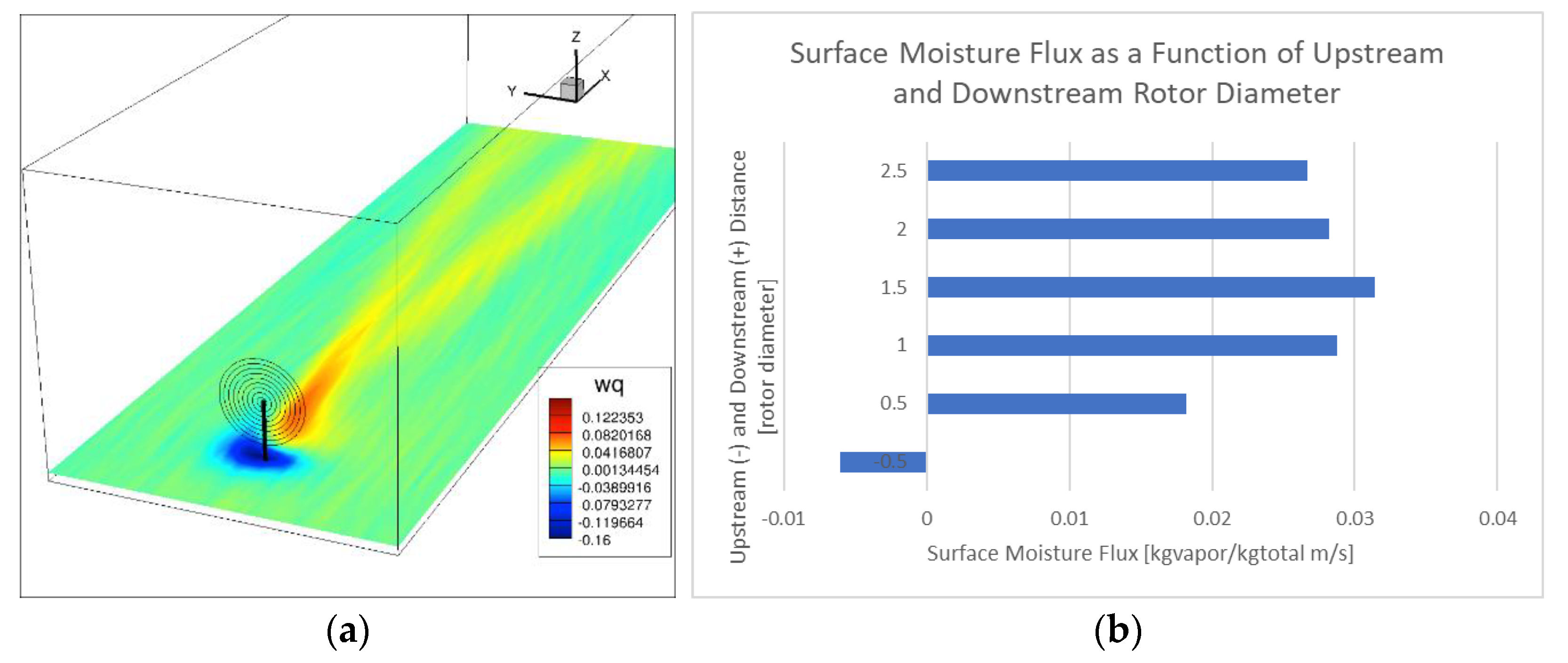
Figure 2.
(a) Contour plots of time-averaged RH change in a vertical plane section passing through the hub and parallel to the streamwise direction; (b) LES time-averaged output and observed changes in RH, as a function of height (reprinted with permission from [36].
Figure 2.
(a) Contour plots of time-averaged RH change in a vertical plane section passing through the hub and parallel to the streamwise direction; (b) LES time-averaged output and observed changes in RH, as a function of height (reprinted with permission from [36].

Figure 3.
(a) Contour plots of time-averaged RH difference in vertical plane slices at fixed downstream distances within a staggered array; (b) Variation of the RH with vertical direction (reprinted with permission from [36]).
Figure 3.
(a) Contour plots of time-averaged RH difference in vertical plane slices at fixed downstream distances within a staggered array; (b) Variation of the RH with vertical direction (reprinted with permission from [36]).

Figure 4.
Wind farm layout and the shadow region in the downstream.

Figure 5.
(a) Iso-surfaces of Q criterion colored by the streamwise velocity component for a 6 × 7 wind farm; (b) contours of mean RH variation in the shadow region (reprinted with permission from [52]).
Figure 5.
(a) Iso-surfaces of Q criterion colored by the streamwise velocity component for a 6 × 7 wind farm; (b) contours of mean RH variation in the shadow region (reprinted with permission from [52]).

Publisher’s Note: MDPI stays neutral with regard to jurisdictional claims in published maps and institutional affiliations. |
© 2022 by the authors. Licensee MDPI, Basel, Switzerland. This article is an open access article distributed under the terms and conditions of the Creative Commons Attribution (CC BY) license (https://creativecommons.org/licenses/by/4.0/).
Share and Cite
MDPI and ACS Style
Adkins, K.A.; Sescu, A. Wind Farms and Humidity. Energies 2022, 15, 2603. https://doi.org/10.3390/en15072603
AMA Style
Adkins KA, Sescu A. Wind Farms and Humidity. Energies. 2022; 15(7):2603. https://doi.org/10.3390/en15072603
Chicago/Turabian StyleAdkins, Kevin A., and Adrian Sescu. 2022. "Wind Farms and Humidity" Energies 15, no. 7: 2603. https://doi.org/10.3390/en15072603
Note that from the first issue of 2016, this journal uses article numbers instead of page numbers. See further details here.