Influence of Natural Convection and Volume Change on Numerical Simulation of Phase Change Materials for Latent Heat Storage

Abstract

For the numerical simulation of a heat storage based on phase change materials (PCMs) an enhanced model is presented, considering the physical effects of convection flow in the liquid phase as well as the volume change during phase change. A modified heat capacity is used to realize the phase change. The phase change material is initially defined as a liquid with temperature-dependent material properties. A volume force is added to the Navier-Stokes equations to allow a circulating flow field in the liquid phase and prevent flow motion in the solid phase. The volume change is implemented with the Arbitrary Lagrangian-Eulerian method. A laboratory phase change experiment was performed using the PCM RT42 with a melting temperature of 42 °C. The laboratory experiment was calculated numerically using the enhanced model to evaluate the numerical model and to investigate the influence of the simulation parameters on the thermal behavior of the PCM. The thermal conductivity is determined as the main influencing parameter. A good agreement of the simulated melting front throughout a major part of the laboratory experiment has been shown. COMSOL Multiphysics provides a default model for phase change, which neglects convection flow and volume change. Compared to the default model, the enhanced model achieves more accurate results but requires more computational cost for complex latent heat storage systems. Using the default model without convection can be reasonable, considering that the heat storage design is either over-dimensioned or a suitable correction factor must be applied.

1. Introduction

Phase change materials are well-suited for heat storage and heat management systems since latent heat is absorbed or released at a constant temperature during the phase change. Therefore, a significantly higher heat quantity is available compared to mere sensible heating. Technical applications of PCM as heat storage are, for example, air conditioning or peak load reduction. PCMs can also be used as buffer storage for solar systems and waste heat utilization, as well as for passive thermal management of battery systems [1,2].

Numerical simulation is an important tool for designing systems with PCM in order to perform optimization without time-consuming and cost-intensive tests. Numerical models of a PCM during phase change require high computational cost due to the occurring physical effects. To reduce the computational effort, simplifications can be made by neglecting certain physical effects. This study investigates the influence of the most used simplifications in numerical phase change models on the accuracy of the numerical results by comparing the results of a laboratory experiment with two different numerical models.

The physical effects during the phase change of a PCM are shown in Figure 1 as a schematic illustration. It shows the section through a cube filled with solid PCM, which is heated from one side with a heat source. The melting occurs starting from this heat source as soon as the temperature of the PCM exceeds the melting temperature. The illustrated physical effects during phase change apply to PCMs regardless of their specific melting temperature. Heat conduction occurs through the entire system towards the lower temperature. Besides, free convection and heat radiation to the environment takes place. Small differences in density in the liquid phase of the PCM occur due to different temperatures. Hence, a convection flow in the liquid fraction of the PCM develops. In this example, a clockwise convection flow is created, resulting in a faster melting of the top areas. A significant change in volume of up to 15 % occurs during the phase change process of a PCM due to the differences in density in the solid and liquid phases. In [3], the modeling of the volume change during phase change is presented with the software ANSYS Fluent with the Volume-of-Fluid method, which is used with a finite-volume discretization. This approach cannot be implemented with the software COMSOL Multiphysics, since COMSOL is based on the finite element method. The volume change is neglected in all present studies regarding numerical modeling of phase change with the software COMSOL Multiphysics. The Marangoni effect describes a temperature-dependent surface tension, resulting in a fluid flow along the surface. This effect can be neglected [4].

Accounting for the effect of the natural convection in the liquid phase requires a coupled system of equations for heat transfer and fluid flow. This results in large computational time [3]. One of the first numerical investigations of phase change with consideration of natural convection was performed by Voller et al. [5]. The numerical model must allow a fluid flow in the liquid phase of the PCM and prevent the flow in the solid part. An easy approach would be to increase the dynamic viscosity in areas with temperatures smaller than the phase change temperature to values which correspond to a solid material. The work of [6] shows that no convergence can be achieved with this approach using COMSOL Multiphysics. The so-called enthalpy–porosity method describes a solution for implementing phase change with natural convection and was first published in [7]. The method is applied in various recent work, for example in [8,9,10,11,12,13] as well as in this paper.

The software COMSOL Multiphysics includes a PCM module which neglects convection flow and volume change. This model will be called default model. However, the physical effects of convection and volume change have a decisive influence on the melting process, as shown above.

In this study, an enhanced numerical PCM model for COMSOL Multiphysics 5.5 is presented, which takes the convection flow in the liquid phase of the PCM and the volume change into account. This model will be called enhanced model in the following. An evaluation of the enhanced model is performed by a numerical recalculation of a performed laboratory experiment. The results are compared to the default model and the application of the numerical models for designing heat storage with PCM is discussed.

2. Materials and Methods

2.1. PCM Selection

The PCM RT42 with a melting temperature of 42 °C is used. The manufacturer’s specifications of the Paraffin RT42 [14] and its thermal volume expansion coefficient [15] are listed in

Table 1. Standard material properties RT42.

Phase change temperature	${\vartheta }_{pc}$	42 °C
Latent heat	$L$	144 kJ/kg
Specific heat capacity	$c_{p,s},c_{p,l}$	2 kJ/(kg·K)
Density, solid phase (15 °C)	${\mathsf{\rho }}_s$	880 kg/m³
Density, liquid phase (80 °C)	${\mathsf{\rho }}_l$	760 kg/m³
Volume expansion	$\mathrm{\Delta }V$	13.6 %
Thermal conductivity	${\mathsf{\lambda }}_s,{\mathsf{\lambda }}_l$	0.2 W/(m·K)
Phase change temperature range	${\mathrm{\Delta }\mathrm{T}}_{pc}$	6 K
Dynamic viscosity	${\mathsf{\mu }}_l$	1.8 mPa·s
Thermal volume expansion coefficient	$\mathsf{\beta }$	0.0001 1/K

.

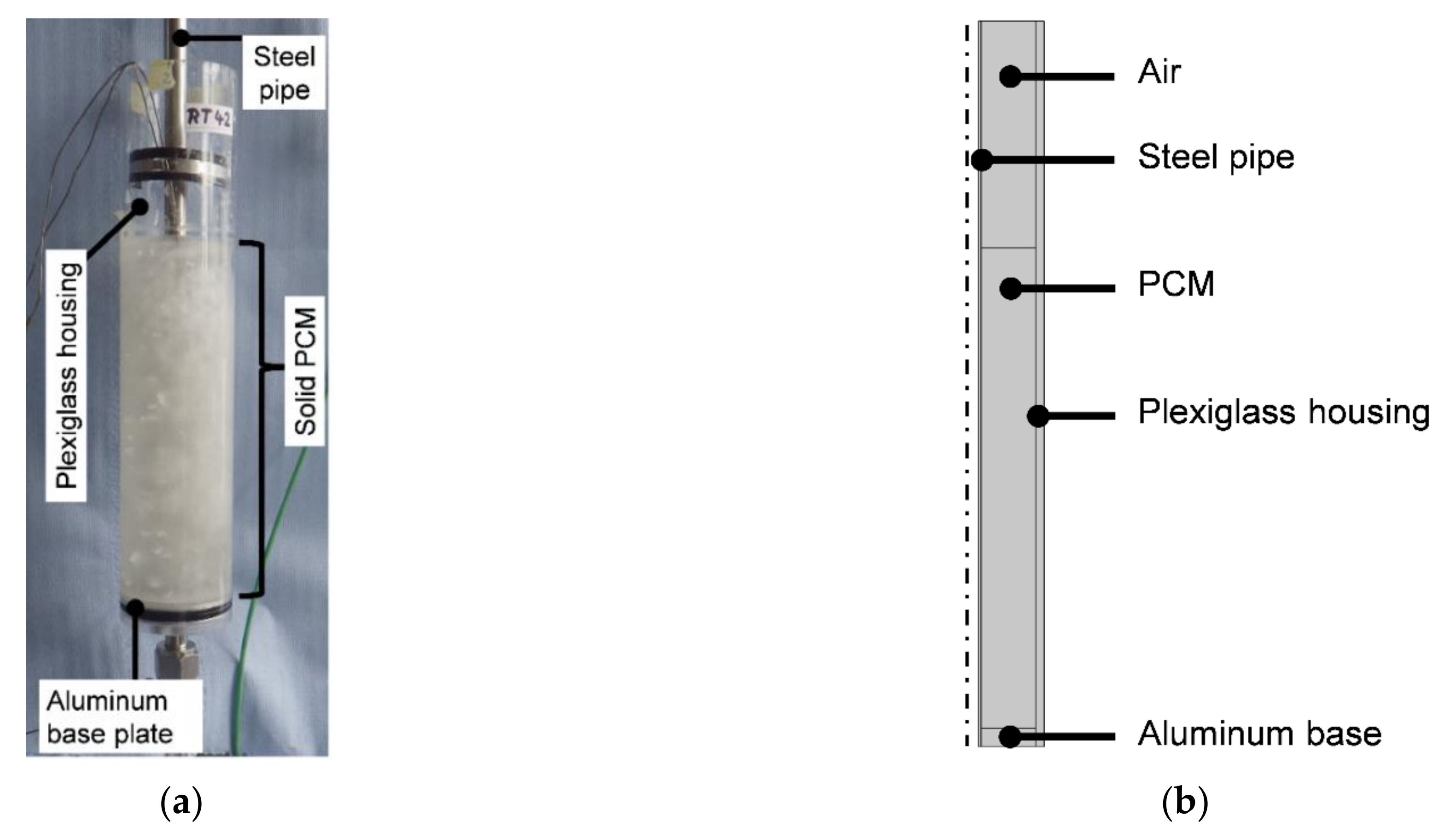
2.2. Experimental Setup

Figure 2a shows the setup of the laboratory experiment consisting of an open upward cylindrical container filled with the PCM RT42, an outer wall made of plexiglass and an aluminum bottom plate. A steel pipe runs vertically centered within the housing and is connected to an upward water flow. The water is tempered to approximately 60 °C at the inlet. The PCM has a height of 18 cm, the air layer has a height of 8.5 cm, and the outer radius of the enclosure is 2.9 cm.

In preparation for the laboratory experiment, the PCM is completely melted and cooled back down to room temperature to minimize air inclusions, which are a result of filling the solid PCM in the cylinder. The ambient temperature is constant at 20 °C. In the beginning, the PCM is entirely in the solid phase. During the melting process a measuring template is used to determine the position of the melting front by measuring distances from the top surface of the PCM at specific times. Only the melting front, which is accessible from the top opening of the cylinder, is measurable with this measuring method. The time for a complete phase change is 255 min and a final volume expansion of 3.2 % is measured afterwards. The manufacturer specifies a volume change of 13.6 % for a temperature range between 15 °C and 80 °C, whereas a significantly smaller temperature range is investigated in the laboratory experiment between 20 °C and 60 °C. Nevertheless, the discrepancy to the material data is large and the volume change is smaller than expected. The results of the experiment such as the melting front are described later.

2.3. Numerical Model

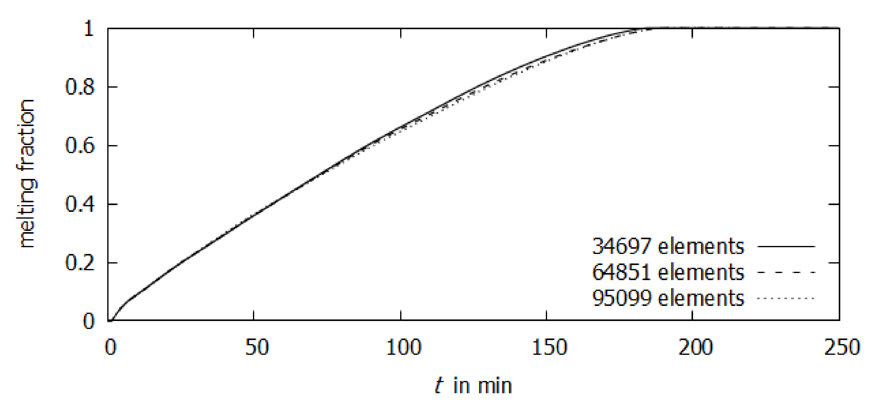
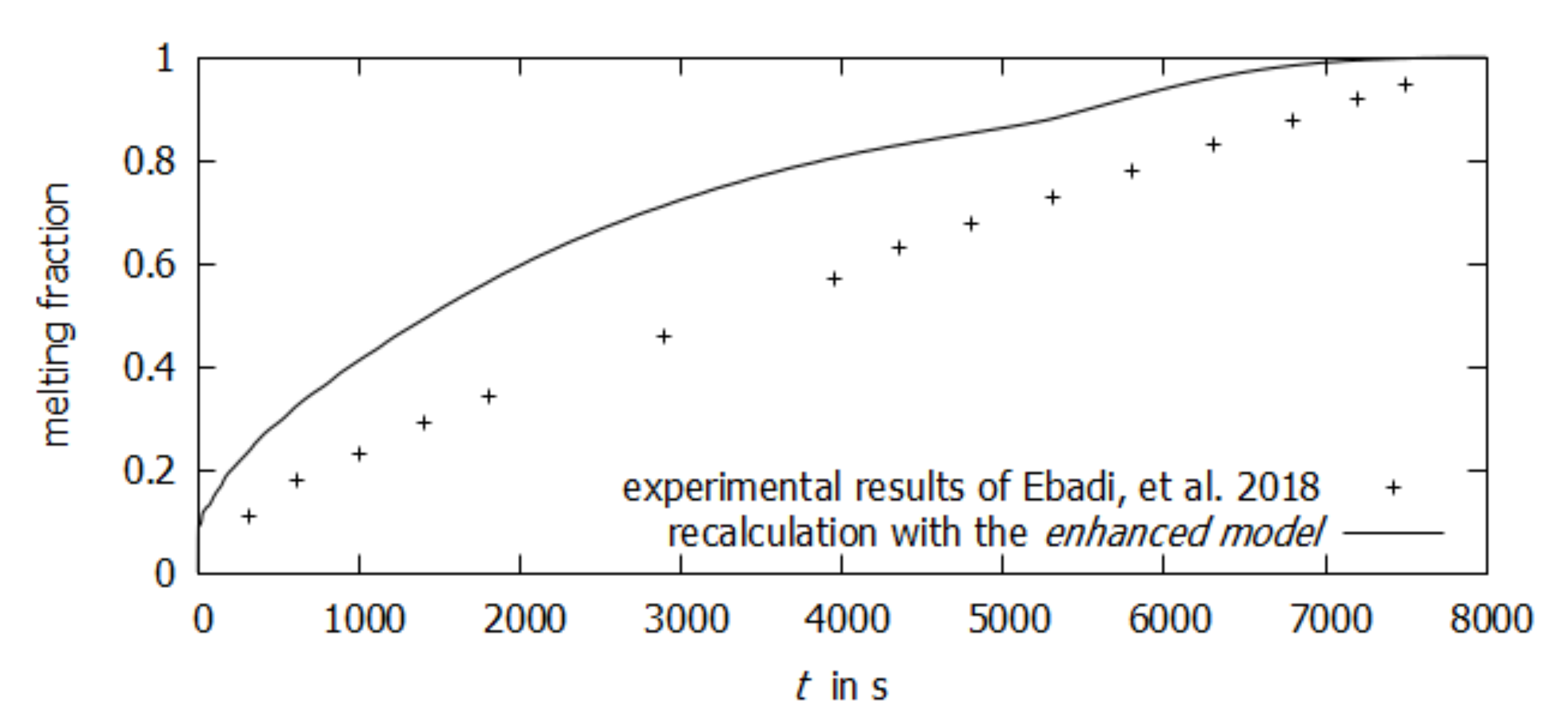
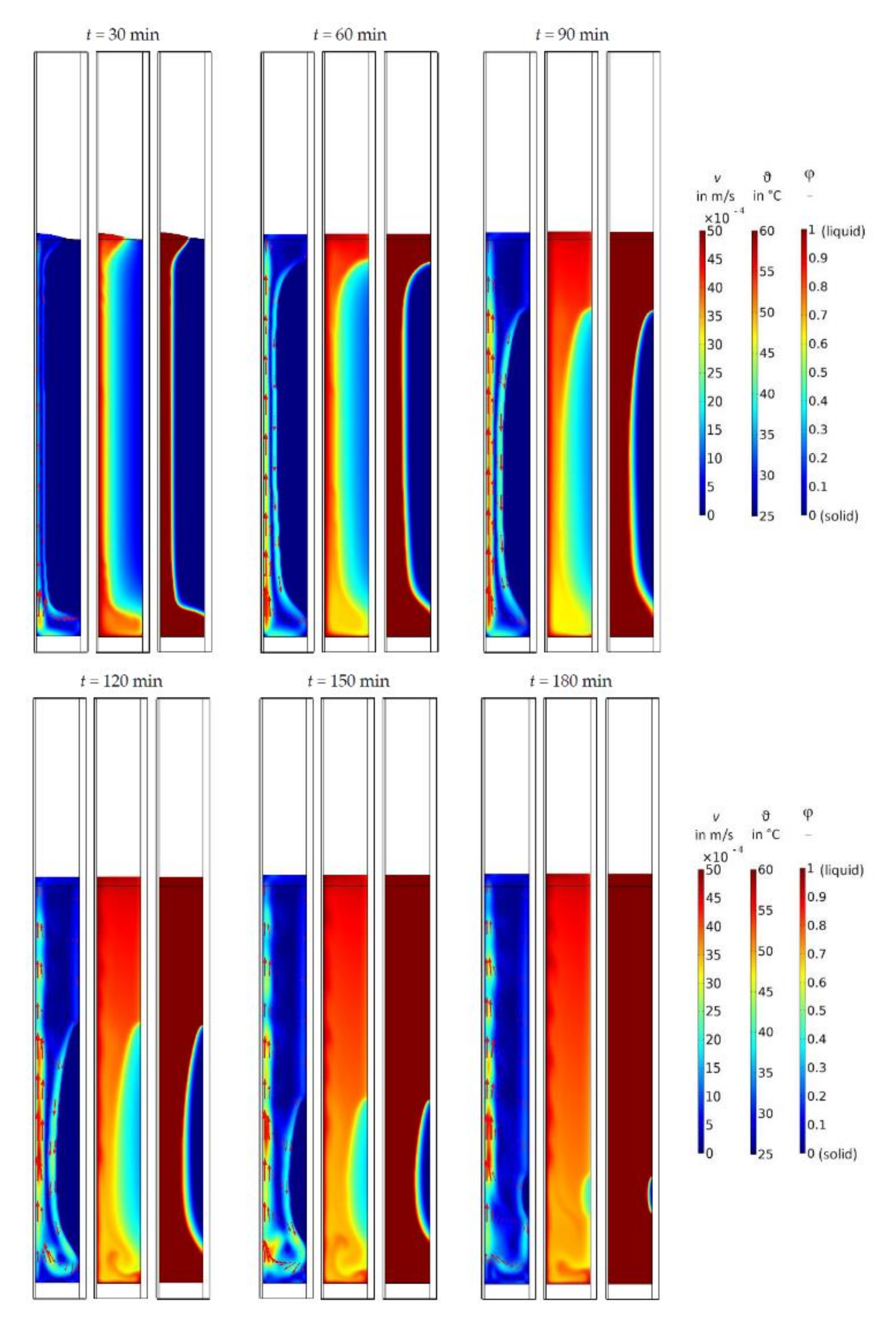
Figure 2b shows the setup of the numerical model. The geometry represents the laboratory experiment, which is modeled two-dimensional and rotationally symmetric. The water flow is represented by a time-dependent temperature boundary condition, which corresponds to the measured and averaged water temperature in the laboratory experiment. To recalculate the laboratory experiment, a density difference is used which corresponds to the measured volume expansion of 3.2 %. Therefore, the assumption of a linear characteristic of density is made between the given values of 15 °C and 80 °C. The influence of different densities while maintaining a constant density difference for the solid and liquid phase is investigated. No significant differences in the results were found. Hence, the densities were set to 825 kg/m³ for the liquid phase and 852 kg/m³ for the solid phase corresponding to temperatures of 45 °C for the liquid phase and 30 °C for the solid phase.

COMSOL Multiphysics provides modules for modeling heat transfer and fluid flow which were used in this study. The boundary conditions correspond to the laboratory experiment. The heat transfer coefficient $\mathsf{\alpha }$ describes the heat flux from surface areas to the environment. Free convection and radiation are considered according to DIN EN ISO 6946, and in this case $\mathsf{\alpha }$ is defined as 7.69 W/(m²$·$K).

A Navier–Slip wall condition was applied to the horizontal outer walls of the PCM as required in [16] for walls next to moving meshes. For the computation, a surface tension$\mathsf{\sigma }$ needs to be specified and the values for Paraffin are between 19 mN/m and 35 mN/m [17]. Preliminary studies have shown that the impact of the magnitude of the surface tension in the given range is neglectable. Thus, the surface tension $\mathsf{\sigma }$ is set to 30 mN/m. Slip wall condition was applied to all remaining walls.

The mesh is generated with triangular elements. The phase transition region needs to be resolved by a sufficient amount of small elements which leads to high computational cost. A grid independency study was performed for three different mesh sizes regarding the overall melting time. The results are shown in Figure 3. The grid with 34,697 elements is chosen due to its good results with a reasonable computation time.

Melting is a time-dependent process, so therefore a transient numerical modeling is necessary. Adaptive time stepping and a fully coupled approach was used, which solves the nonlinear system of equations as a single large system of equations within one iteration [18].

The fundamental theory described in the following section can be found in [18]. The description of the temperature field follows from conservation of energy to Equation (1).

$$\rho c_p\frac{\partial T}{\partial t}+\rho c_p\mathit{u}\cdot \mathit{\nabla }T+\mathit{\nabla }\cdot \left(\dot{{\mathit{q}}_{\mathit{c}}}+\dot{{\mathit{q}}_{\mathit{r}}}\right)=\beta T\left(\frac{\partial p}{\partial t}+\mathit{u}\cdot \mathit{\nabla }p\right)+\tau :\mathit{\nabla }\mathit{u}+Q$$

(1)

The numerical model for solving the flow field is based on the basic equations of fluid mechanics according to [19]. The Navier–Stokes equations for an incompressible flow with a Newtonian fluid are shown in Equations (2) and (3). An additional term $-S\left(T\right)\cdot \mathit{u}$, which is described later, is necessary to model the transition area between the solid and liquid phases.

$$\rho \mathit{\nabla }\cdot \mathit{u}=0$$

(2)

$$\rho \frac{\partial \mathit{u}}{\partial t}+\rho \left(\mathit{u}\cdot \mathit{\nabla }\right)\mathit{u}=\mathit{\nabla }\cdot \left[-p\mathit{I}+\mu \left(\mathit{\nabla }\mathit{u}+{\left(\mathit{\nabla }\mathit{u}\right)}^T\right)\right]+{\mathit{F}}_{\mathit{B}}-S\left(T\right)\cdot \mathit{u}$$

(3)

The buoyancy force ${\mathit{F}}_{\mathit{B}}$ causes the natural convection in the liquid phase and is calculated using the Boussinesq approximation according to Equation (4), with the magnitude of the acceleration of gravity $\mathit{g}$ of 9.81 m/s².

$${\mathit{F}}_{\mathit{B}}=-{\rho }_l\cdot \beta \cdot \mathit{g}\cdot \left(T-T_{pc}\right)$$

(4)

The phase change is characterized by the melting fraction φ according to Equation (5). The parameter phase change temperature range $\mathrm{\Delta }{T}_{pc}$ defines the range of the transition area.

$$\begin{array}{l}\phi \left(T\right)=0\mathrm{for} T<T_{pc}-\frac{\mathrm{\Delta }{T}_{pc}}{2}\\ \phi \left(T\right)=\frac{T-\left(T_{pc}-\frac{\mathrm{\Delta }{T}_{pc}}{2}\right)}{\mathrm{\Delta }{T}_{pc}}\mathrm{for} T_{pc}-\frac{\mathrm{\Delta }{T}_{pc}}{2}<T<T_{pc}+\frac{\mathrm{\Delta }{T}_{pc}}{2}\\ \phi \left(T\right)=1\mathrm{for} T<T_{pc}+\frac{\mathrm{\Delta }{T}_{pc}}{2}\end{array}$$

(5)

To describe the convection flow in the liquid phase, the so-called enthalpy porosity method is used to allow convection flow in the liquid phase while preventing flow in the solid PCM. Therefore, an additional source term $S\left(T\right)$is defined according to Equation (6), which contains the Carman–Kozeny relation. The so-called mushy zone factor Am is important for numerical modelling and its magnitude has a decisive influence on the results and is described below. The constant $ϵ$ = 0.001 prevents division by zero for the case $\phi \left(T\right)$ = 0.

$$S\left(T\right)=A_m\frac{{\left(1-\phi \left(T\right)\right)}^2}{\phi {\left(T\right)}^3+ϵ}$$

(6)

The source term $S\left(T\right)$approaches zero for liquid areas with a melting fraction of $\phi \left(T\right)$ = 1. This results in a flow corresponding to the standard Navier–Stokes equations. Solid areas and the transition area have a melting fraction $\phi \left(T\right)$< 1, which leads to a great value of the source term $S\left(T\right)$depending on the magnitude of the mushy zone factor Am. Therefore, the fluid flow is prevented in the solid area and reduced in the transition area between solid and liquid phase.

The best results are achieved by using great magnitudes for the mushy zone factor. Preliminary studies have shown that there is no significant change in the results for $A_m\ge 1·{10}^4$kg/(m³$·$s) for incompressible flows. In this paper, the mushy zone factor $A_m=1·{10}^4$ kg/(m³$·$s) is used, thus convergence is achieved for compressible flow.

The volume change is solved using the Arbitrary Lagrangian–Eulerian method. It describes the motion of a surface which divides the air and the PCM [18]. In COMSOL Multiphysics, this can be added by the “Moving Mesh” module with a deformable geometry for the two domains PCM and air.

The physics of phase transformation is implemented according to [11] with user-defined functions and material properties. The PCM is treated numerically as a liquid. User-defined functions are used to describe the material properties of the solid and liquid PCM as well as the flow in the transition zone. The melting fraction $\phi \left(T\right)$is used to describe temperature-dependent material properties. The density $\rho \left(T\right)$ is obtained according to Equation (7) and the thermal conductivity $\lambda \left(T\right)$ similarly, according to Equation (8).

$$\rho \left(T\right)={\rho }_s+\left({\rho }_l-{\rho }_s\right)\cdot \phi \left(T\right)$$

(7)

$$\lambda \left(T\right)={\lambda }_s+\left({\lambda }_l-{\lambda }_s\right)\cdot \phi \left(T\right)$$

(8)

To define the phase-dependent viscosity $\mu \left(T\right)$, the source term $S\left(T\right)$ is used as well as an auxiliary constant $\xi$= 1 m², as shown in Equation (9).

$$\mu \left(T\right)={\mu }_l+S\left(T\right)\cdot \xi$$

(9)

The heat capacity method defines the phase change using a modified specific heat capacity. The latent heat is the characteristic quantity for the phase change. A Gaussian function according to Equation (10) is used, which is centered around the phase change temperature $T_{pc}$.

$$D\left(T\right)=\frac{e^{-\frac{{\left(T-T_{pc}\right)}^2}{{\left(\mathrm{\Delta }{T}_{pc}/4\right)}^2}}}{\sqrt{\pi {\left(\mathrm{\Delta }{T}_{pc}/4\right)}^2}}$$

(10)

The modified specific heat capacity $c_p\left(T\right)$ is calculated according to Equation (11), maintaining the energy balance during phase change.

$$c_p\left(T\right)=c_{p,s}+\phi \left(T\right)\cdot \left(c_{p,l}-c_{p,s}\right)+L\cdot D\left(T\right)$$

(11)

The validation of the enhanced model was done by recalculating the experiment presented in [20]. Figure 4 shows a good agreement of the overall melting time.

3. Results

The numerical results of the velocity $v$, the temperature $\vartheta ,$ and the melting fraction$\phi$ are shown in Figure 5 for the enhanced model. Only the PCM domain is visualized. The influence of the convection flow in the upper region of the PCM can be seen in the curved phase boundary between the solid and liquid phase, resulting in a faster melting of the upper regions of the PCM. In addition, due to the high thermal conductivity of the aluminum bottom plate, melting starts at the bottom. The volume expansion of the PCM into the air domain results from the density difference between the solid and liquid PCM.

Additionally, the measured position of the melting front of the laboratory experiment for three different time points are marked with white triangles in Figure 6. The number of measured points differ between different times due to the measurement method described in Section 2.2. Melting starting from the bottom plate is represented by one measuring point at the bottom. The position of the melting front in between the top and bottom measuring points is not measurable.

Until 120 min approximately 75 % of the PCM is melted and there is a good agreement in the position and shape of the melting front between the laboratory experiment and the simulation. The melting of the last 25 % of the PCM required 135 min in the laboratory experiment but only 65 min in the simulation.

A parameter study was performed to investigate the influence of the following simulation parameters on the overall melting time $t_{pc}$: the specific heat capacity $c_{p,s}$ and ${\mathrm{c}}_{\mathrm{p},\mathrm{l}}$, the phase change temperature range $\mathrm{\Delta }{T}_{pc}$, the thermal expansion coefficient $\beta$, the latent heat $L$, the heat transfer coefficient $\alpha$, and the thermal conductivity $\lambda$. The investigated parameters are individually increased or decreased by 20 %. The change of the melting time $\mathrm{\Delta }{t}_{pc}$ compared to the enhanced model with a melting time $t_{pc}$ of 184 min is studied. The latent heat $L$, the heat transfer coefficient $\alpha$, and the thermal conductivity $\lambda$ were found to have the greatest influence, which is shown in

Table 2. Parameter study: Influence of different parameters on the melting time$t_{pc}$. The change of the melting time $\mathrm{\Delta }{t}_{pc}$ refers to the enhanced model with$t_{pc}=184\min .$

Parameter	Parameter Change of −20%$\mathbf{\Delta }{\mathit{t}}_{\mathit{p}\mathit{c}}$		Parameter Change of +20%$\mathbf{\Delta }{\mathit{t}}_{\mathit{p}\mathit{c}}$
$\mathrm{Thermal}\mathrm{conductivity}\lambda$	+29.7 %	+54.8 min	−17.0 %	−31.3 min
$\mathrm{Heat}\mathrm{transfer}\mathrm{coefficient}\alpha$	−8.1 %	−15.0 min	+16.5 %	+30.6 min
$\mathrm{Latent}\mathrm{heat}L$	−14.4 %	−26.5 min	+15.8 %	+29.1 min

.

The values used for the latent heat and the heat transfer coefficient can be considered as reliable data. The thermal conductivity $\lambda$ has the greatest influence on the melting time$t_{pc}$. In general, there is a temperature and phase dependency for the thermal conductivity [21], which is unknown for the used PCM RT42. Moreover, small air inclusions occur in the PCM during the solidification process in the laboratory experiment, which leads to a decreased thermal conductivity. Therefore, a deviation of the manufacturer’s data from the real thermal conductivity is possible. In this case, fast charging of the heat storage is achieved by melting 75 % of the PCM and an insulation around the heat storage is recommended additionally.

Another numerical calculation of the laboratory experiment is made using the default model, which is available in COMSOL and neglects convection flow and volume change. Figure 7 shows the numerical results of the default model (a) and of the enhanced model (c) after 120 min. In the default model the melting front is vertical to the heat source, and no complete melting of the PCM occurs. This is a discrepancy to the results of the laboratory experiment and to the enhanced model. Therefore, a latent heat storage designed with the default model leads to an over-dimensioned thermal energy storage system. The default model and the enhanced model show the same results during the solidification process.

4. Discussion

The numerical calculation of a performed laboratory experiment shows that the physics of the phase change is well represented with the enhanced model until 75 % of the PCM has been melted. The melting duration of the last 25 % of the PCM is not represented correctly in the enhanced model. Therefore, in this setup it is recommended to avoid melting the last 25 % of the PCM and to add an insulation to achieve faster melting. The limitation of the enhanced model is large computational costs. The implementation of the enhanced model leads to an increase of the computational time by a factor of 60 compared to the default model due to complex flow calculation.

The default model is suited for the design of heat storages with large dimensions because it is easy to implement for complex geometries and has low computational costs. For melting, the melting fraction is represented inaccurately due to the neglection of the convection flow in the liquid PCM and the volume change. This leads to the design of over-dimensioned latent heat storage with the default model. To compensate for the neglected physical effects of the default model, the use of a correction factor is recommended to avoid an over-dimensioned storage. The aim of using a factor is a good agreement of the average melting fraction of the default model and the laboratory experiment. The thermal conductivity is suitable because it has the greatest influence on the melting process. The value of the factor is not universal but depends on the operating conditions like the PCM and the geometry. A further parameter study found that a multiplication of the thermal conductivity by the factor 2 results in a good representation of the laboratory experiment with the PCM RT42. Figure 7b shows the melting fraction of the default model with factor 2 after 120 min. The increased thermal conductivity leads to faster melting. This will not result in a correct shape of the melted PCM, but it compensates the neglected influence of the convection flow on the heat transfer rate. As a result, the melting fraction of the system and the required melting time can be calculated. Further investigations of the correction factor for PCMs with different melting temperatures are suggested.

References

1. Hübner, S. Techno-Ökonomische Optimierung Eines Hochtemperatur-Latentwärmespeichers. Ph.D. Thesis, University of Stuttgart, Stuttgart, Germany, 2018. [Google Scholar]
2. Kötter, T. Hochleistungsdichte Phasenwechsel-Komposit-Materialien für das Thermische Management Elektrotechnischer Systeme. Ph.D. Thesis, Friedrich-Alexander Universität Erlangen-Nürnberg, Erlangen, Germany, 2017. [Google Scholar]
3. Vogel, J. Influence of Natural Convection on Melting of Phase Change Materials. Ph.D. Thesis, University of Stuttgart, Stuttgart, Germany, 2019. [Google Scholar]
4. Sedeh, M.; Khodadadi, J. Solidification of phase change materials infiltrated in porous media in presence of voids. J. Heat Transf. 2014, 136, 112603. [Google Scholar] [CrossRef]
5. Voller, V.R. An enthalpy method for convection/diffusion phase change. Int. J. Numer. Methods Eng. 1987, 24, 271–284. [Google Scholar] [CrossRef]
6. Samara, F.; Groulx, D.; Biwole, P.H. Natural convection driven melting of phase change material: Comparison of two methods. In Proceedings of the COMSOL Conference in Boston, Newton, MA, USA, 3–5 October 2012. [Google Scholar]
7. Voller, V.R.; Prakash, C. A fixed grid numerical modelling methodology for convection-diffusion mushy region phase-change problems. Int. J. Heat Mass Transf. 1987, 30, 1709–1719. [Google Scholar] [CrossRef]
8. Coulson, R. Numerical Modeling of a Lead Melting Front under the Influence of Natural Convection. Master’s Thesis, Colorado School of Mines, Golden, CO, USA, 2013. [Google Scholar]
9. Goyal, P.; Dutta, A.; Verma, V.; Thangamani, I.; Singh, R.K. Enthalpy porosity method for CFD simulation of natural convection phenomenon for phase change problems in the molten pool and its importance during melting of solids. In Proceedings of the Comsol Conference in Bangalore, Bangalore, India, 18 October 2013. [Google Scholar]
10. Groulx, D.; Biwole, P.H. Solar PV passive temperature control using phase change materials. In Proceedings of the 15th International Heat Transfer Conference, Kyoto, Japan, 10–15 August 2014. [Google Scholar]
11. Kheirabadi, A.C.; Groulx, D. Simulating phase change heat transfer using COMSOL and FLUENT: Effekt of the mushy-zone constant. Comput. Therm. Sci. 2015, 7, 427–440. [Google Scholar] [CrossRef]
12. Kheirabadi, A.C.; Groulx, D. The effekt of the mushy-zone constant on simulated phase change heat transfer. In Proceedings of the ICHMT International Symposium on Advances in Computational Heat Transfer, New Brunswick, NJ, USA, 25–29 May 2015. [Google Scholar]
13. Rubinetti, D.; Weiss, D.A. Modeling approach to facilitate thermal energy management in buildings with phase change materials. In Proceedings of the COMSOL Conference in Lausanne, Lausanne, Switzerland, 22–24 October 2018. [Google Scholar]
14. Material Data Sheet, PCM RT42 (Rubitherm GmbH). Available online: https://www.rubitherm.eu/index.php/produktkategorie/organische-pcm-rt (accessed on 1 February 2022).
15. Sathe, T.M.; Dhoble, A.S. Thermal management of low concentrated photovoltaic systems using extended surfaces in phase change materials. J. Renew. Sustain. Energy 2018, 10, 043704. [Google Scholar] [CrossRef]
16. COMSOL Multiphysics 5.5: Microfluids Module User’s Guide. Available online: https://doc.comsol.com/5.5/doc/com.comsol.help.mfl/MicrofluidicsModuleUsersGuide.pdf (accessed on 1 February 2022).
17. Kneer, A.; Nestler, B.; Bantle, B.; Kotitschke, T. Entwicklung und Erprobung eines auf Metallschaum basierenden Systems (Demonstrator) zur regenerativen Nutzung und Speicherung von Abwärme aus Energiegewinnungsprozessen. 2012. Available online: https://pudi.lubw.de/detailseite/-/publication/22381 (accessed on 1 February 2022).
18. COMSOL Multiphysics 5.5: Reference Manual. Available online: https://doc.comsol.com/5.5/doc/com.comsol.help.comsol/COMSOL_ReferenceManual.pdf (accessed on 1 February 2022).
19. Oertel, H. (Ed.) Prandtl—Führer durch Die Strömungslehre: Grundlagen und Phänomene; Springer Vieweg: Wiesbaden, Germany, 2002. [Google Scholar]
20. Ebadi, S.; Al-Jethelah, M.; Tasnim, S.H.; Mahmud, S. An investigation of the melting process of RT-35 filled circular thermal energy storage system. Open Phys. 2018, 16, 574–580. [Google Scholar] [CrossRef]
21. Mehling, H.; Cabeza, L.F. Heat and Cold Storage with PCM; Springer-Verlag GmbH: Berlin/Heidelberg, Germany, 2008. [Google Scholar]
Figure 1. Schematic illustration of the physical effects of a melting PCM with a heat source at the left side.
Energies 15 02746 g001
Figure 2. (a) Setup of the laboratory experiment. (b) Geometry of the two-dimensional and rotationally symmetric numerical model.
Energies 15 02746 g002
Figure 3. Grid independency study.
Energies 15 02746 g003
Figure 4. Melting fraction of the enhanced model compared to the experimental results of Ebadi, et al. 2018 [20].
Energies 15 02746 g004
Figure 5. Numerical results of the enhanced model for the PCM-domain: Velocity v (left), temperature ϑ (center), and melting fraction φ (right).
Energies 15 02746 g005
Figure 6. Comparison of the experimental results (triangles) and numerical results of the enhanced model (melting fraction φ).
Energies 15 02746 g006
Figure 7. Melting fraction after 120 min: (a) Default model, (b) Default model with factor 2, (c) Enhanced model with convection flow and volume change and the experimental results.
Energies 15 02746 g007