Experimental Analysis of Ultra-High-Frequency Signal Propagation Paths in Power Transformers

Abstract

Ultra-high-frequency (UHF) partial discharge (PD) monitoring is gaining popularity because of its advantages over electrical methods for onsite/online applications. One such advantage is the possibility of three-dimensional PD source localization. However, it is necessary to understand the signal propagation and attenuation characteristics in transformers to improve localization. Since transformers are available in a wide range of ratings and geometric sizes, it is necessary to ascertain the similarities and differences in UHF signal characteristics across the different designs. Therefore, in this contribution, the signal attenuation and propagation characteristics of two 300 MVA transformers are analyzed and compared based on experiments. The two transformers have the same rating but different internal structures. It should be noted that the oil is drained out of the transformers for these tests. Additionally, a simulation model of one of the transformers is built and validated based on the experimental results. Subsequently, a simulation model is used to analyze the electromagnetic wave propagation inside the tank. Analysis of the experimental data shows that the distance-dependent signal attenuation characteristics are similar in the case of both transformers and can be well represented by hyperbolic equations, thus indicating that transformers with the same rating have similar attenuation characteristics even if they have different internal structures.

1. Introduction

Undetected partial discharge (PD) activity is one of the leading causes of failure in power transformers and hence should be detected at the earliest possible stage [1]. Of the many methods to detect PD activity, the ultra-high-frequency (UHF) method has gained popularity in recent years because of advantages such as continuous on-line monitoring, good signal-to-noise ratio, resilience against external disturbances, and the possibility of three-dimensional PD source localization [2,3]. Currently, research is being carried out in the areas of UHF sensor design [4,5,6], PD pattern recognition [7,8], localization algorithms [9,10,11], and calibration of UHF measurements [12,13]. UHF monitoring works on the principle that the PD current pulse, which has a short rise-time (less than 1 ns), results in electromagnetic (EM) waves in the UHF range (300 MHz–3 GHz). The EM waves propagate through the tanks and are detected by UHF sensors installed on the transformer tank. With at least four sensors installed on the tank wall [14], the PD source can be localized using the principle of time difference of arrival (TDOA) of the signals at the different sensors [15]. However, the signal propagation path inside transformers is quite complex. E.g., EM waves cannot travel through the active part of the transformer and travel around it. Additionally, the signals undergo multiple reflections at the tank walls and the active part until their energy is dissipated [16,17]. Therefore, understanding the signal propagation characteristics in transformers is key to improving localization accuracy.

Transformers are available in different sizes and ratings, each one with a different internal structure. It is well known that the active parts influence signal propagation and attenuation [9,16,18]. However, the extent to which differently designed active parts can influence the signals has not been extensively researched using experimental results obtained from transformers [18]. An in-depth analysis of the similarities and differences in signal characteristics across different transformers can greatly aid in improving the accuracy of localization and the development of a generalized signal attenuation model.

Therefore, in this contribution, UHF measurements are conducted on two 300 MVA transmission transformers, which have different internal structures, to compare the signal propagation and attenuation characteristics in both cases. The signals are analyzed in time and frequency domains. Additionally, a simulation model of one transformer is built in CST Microwave Studio to ascertain whether the signal behavior can be replicated and study the electromagnetic wave propagation inside the tank. Since oil had to be drained out of the transformers to enable testing, the dielectric medium in this analysis is air. The impact of oil on signal behavior has been analyzed in previous work using simulation models and has been compared with results obtained in air [19].

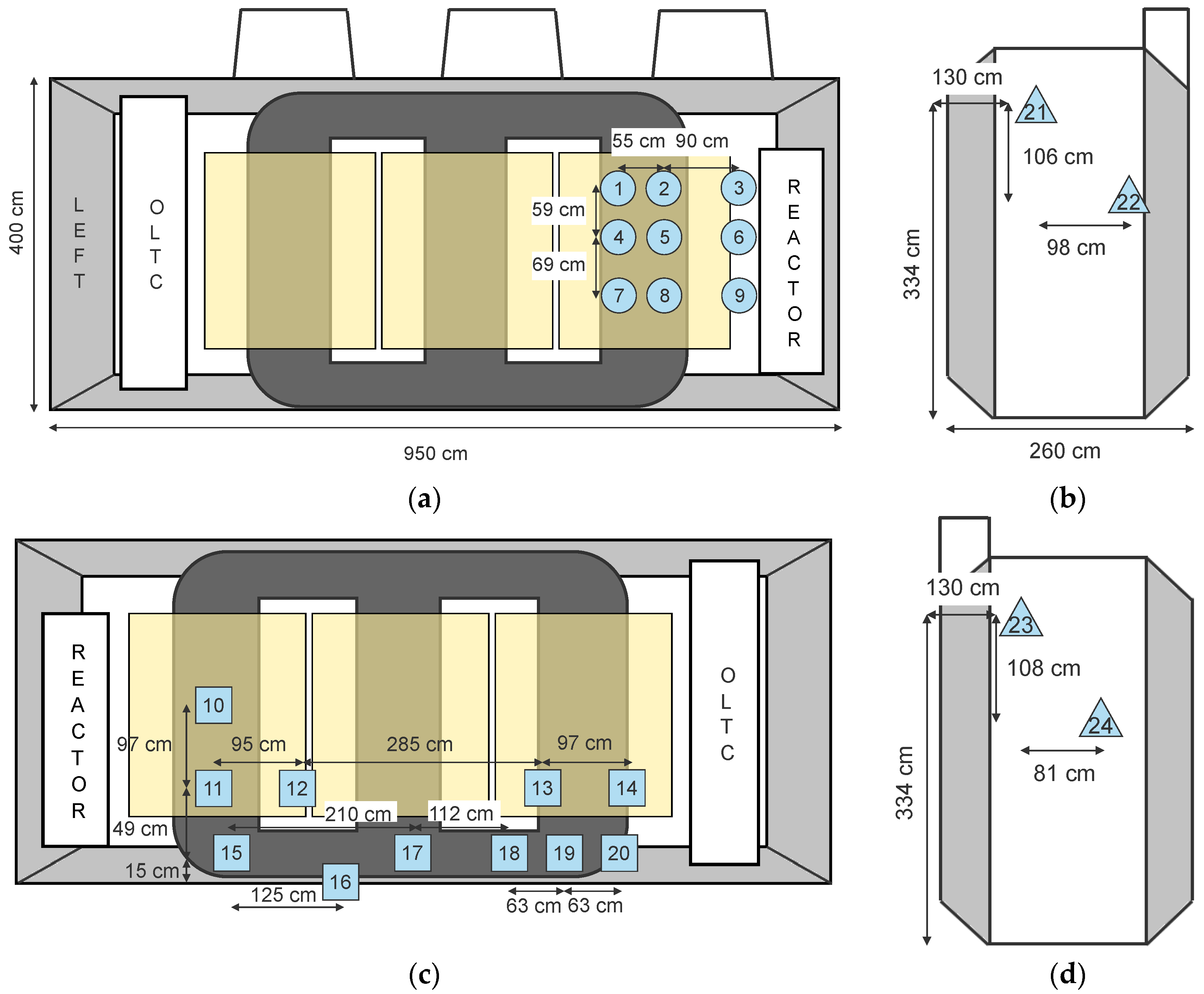
2. Experimental Setup

2.1. Transformer A

Transformer A is a 300 MVA, 420 kV transmission transformer with tank dimensions of 900 × 400 × 260 cm and has a three-limb core and three windings: low- (LV), medium- (MV), and high-voltage (HV). The HV winding also has coarse and fine tap windings. The transformer also has an on-load tap changer (OLTC) and a reactor, which is connected to the LV winding to protect the windings from external overcurrent.

Twenty-four holes were drilled into the tank to install the monopole antennas. Nine monopoles were installed on the front tank wall, five on the rear tank wall, six on the non-orthogonal part at the bottom of the rear tank wall, and four (two each) on the side tank walls. The oil was drained out of the tank in order to drill holes, and testing was carried out in an air-filled tank. The positions of all sensors are shown in Figure 1. A total of 4 sensors were used as sources, and 21 sensors were used as receivers, resulting in 84 measurements. An artificial pulse generator (HFIG 600), with a rise time (10–90%) of 80 ps and a flat curve in the frequency domain up to 1 GHz [20], was used to generate the excitation pulse sent to the monopole antenna, and a signal strength of 60 V was used. The pulse waveform and its frequency spectrum are shown in Figure 2. The time-domain waveform was recorded by connecting the output of the pulse generator to a digital storage oscilloscope (DSO), and the frequency response was measured using a spectrum analyzer.

A DSO with the following specifications was used to record the measurement data: 4 GHz analogue bandwidth, 12.5 GS/s sampling rate, 12-bit vertical resolution, and 50 Ω input impedance. A recording time of 400 ns was used for all measurements. Three channels of the DSO were used. The signal reaching the source antenna was sent to Channel 1 of the DSO using a T-joint. Therefore, Channel 1 acted as the reference signal for all measurements and could be used for time of arrival (ToA) analysis. Channels 2 and 3 were connected to two receiving sensors using coaxial cables of equal lengths. The sensors connected to these two channels were changed until all possible receivers had been used for each source. Sensors 6, 13, 22, and 23 were used as sources, and sensors 1–18 and 21–24 were used as receivers.

2.2. Transformer B

Transformer B is also a 300 MVA, 420 kV transmission transformer with the same tank dimensions. However, there are some key differences in the construction of the active part and internal components as compared to transformer A. Firstly, the core has 5 limbs, and additionally, the reactor is in a different position.

A total of 17 holes were drilled into the tank after the oil had been drained out to install 10 cm long monopole antennas. These antennas have a resonant frequency at 750 MHz, based on results obtained from simulations. Of these antennas, 12 were used as sources, and 13 were used as receivers, resulting in 156 measurements, as described in [21]. The same pulse generator and signal strength were used, albeit with a rectangular pulse [21]. The rectangular pulse has frequency content up to 1 GHz, whereas the pulse used in the test on transformer A has frequency content up to 4 GHz. However, on comparing the frequency spectra of comparable measured UHF signals in the two setups, it was found that there are no significant frequency components above 1 GHz, i.e., the higher frequency components of the shorter pulse are attenuated by the time they reach the receiving sensors [22]. Therefore, the different pulse waveforms do not have a significant effect on the results. Additionally, the sensors were not placed in the same positions as those in transformer A. All details regarding the sensor placement and test setup can be found in [21].

The receivers were connected to a DSO using RG214 coaxial cables of equal length. The DSO has the following specifications: a 4 GHz analogue bandwidth, 20 GS/s sample rate, 8-bit vertical resolution, and 50 Ω input impedance. A recording time of 5 μs was used for all measurements. Three channels were used to measure the signals received by different antennas. Since there was no common reference signal between different measurements, propagation times cannot be analyzed using the data obtained from transformer B.

3. Simulation Setup

A simulation model of transformer B has been validated in previous research [23]. In this contribution, a similar model of transformer A was built in CST Microwave Studio to study the signal propagation and attenuation characteristics [18,24,25,26]. The simulation was carried out in an air-filled tank so as to maintain parity with the measurements. Copper was used as the material for the winding, and a 0.3 mm coating of oil-impregnated paper was used on top of the copper to model the winding insulation. Silicon steel was used as the material for the core.

The gap-feed model was used to simulate the monopole antennas [27,28]. For the source monopole antenna, a voltage port was used in the gap between the base of the antenna and the ground plane (the transformer tank wall). For the receivers, an S-parameter port was used in the gap. All monopoles were modeled as perfect electric conductors (PECs), and a gap of 0.5 mm was used between the base of the conductor and the ground plane. The monopoles were positioned at the same locations as they were in the experiment.

The following simplifications were used to reduce the computational load. Firstly, the layer windings, i.e., the LV winding, coarse winding, and fine winding, were modeled as solid cylinders. Each disk of the disk windings, i.e., the MV and HV windings, was modeled separately; however, the individual turns in a disk were not modeled. Next, additional components such as the on-load tap changer (OLTC) were not modeled to reduce the computational load. Additionally, the individual laminates of the core were not modeled to reduce the number of mesh cells [10,18,28]. The monopoles installed on the slanted walls of the transformer tank could not be simulated at their actual angle of installation, as they had to be aligned to one of the Cartesian planes. Lastly, a maximum frequency limit of 900 MHz was implemented because the majority of the frequency content of measured signals lies within this range. Additionally, mesh refinement was used in the regions around the monopole antennas because the width of the gap was much smaller than the size of the tank. Therefore, the smallest mesh cell in the model had a dimension of 0.25 mm. Overall, the model consisted of approximately 75 million mesh cells after these simplifications and refinements.

The artificial PD signal generated by the pulse generator was used as the input to the simulation model with a signal strength of 60 V (the same as the experiment). The time-domain solver was used to simulate signal propagation with the lowest available accuracy setting of −20 dB. The lowest accuracy setting was used to reduce computation time.

4. Results

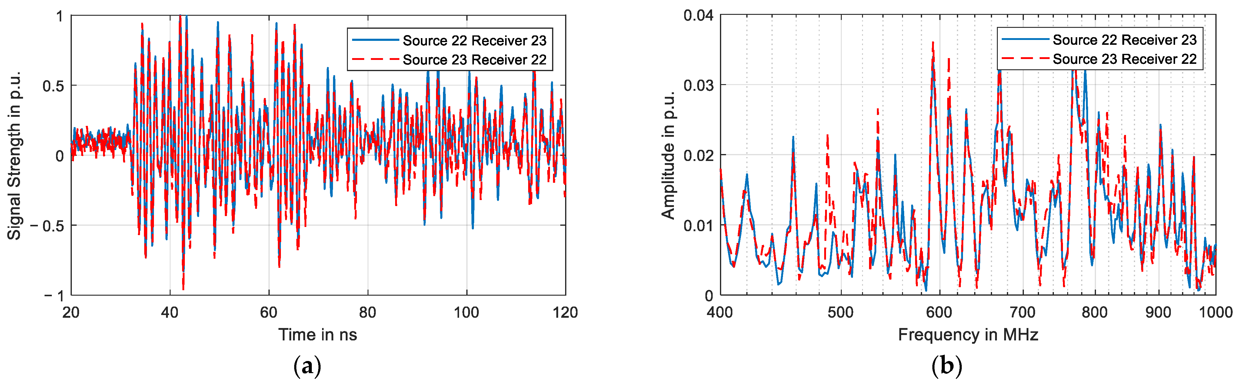
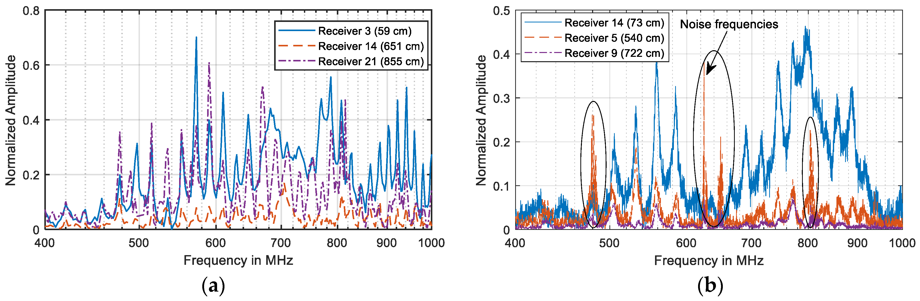
4.1. Basic Signal Analysis

A finding from reversing the source and the receiver is that the signal properties in both cases are very similar. As shown in Figure 3, the time- and frequency-domain signals obtained from transformer A, when two sensors (22 and 23) are interchanged as source and receiver, are almost identical, i.e., both signals have similar time-domain waveforms, ToAs, and frequency spectra. This phenomenon implies that the propagation path remains unchanged between the two scenarios. A reason for the minor differences between the measurements could be some structure inside the transformer that does not behave the same way on both paths. E.g., a hollow hemisphere that acts as a convex surface on one path and as a concave surface on the other, resulting in differences in measured signals.

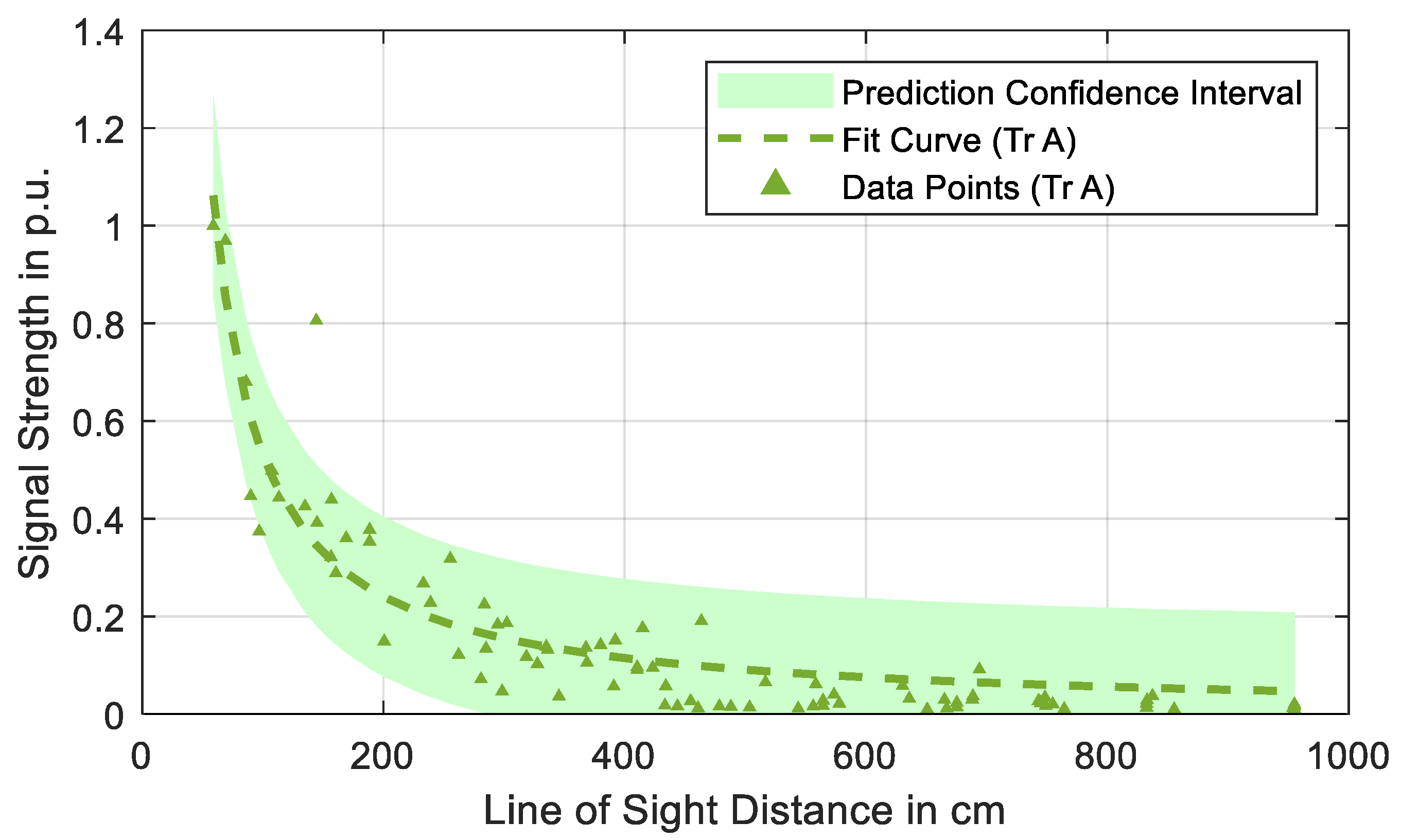
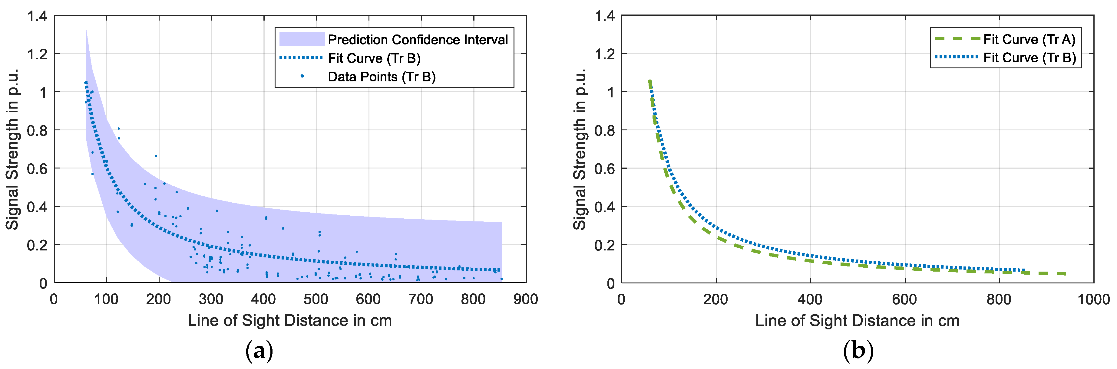
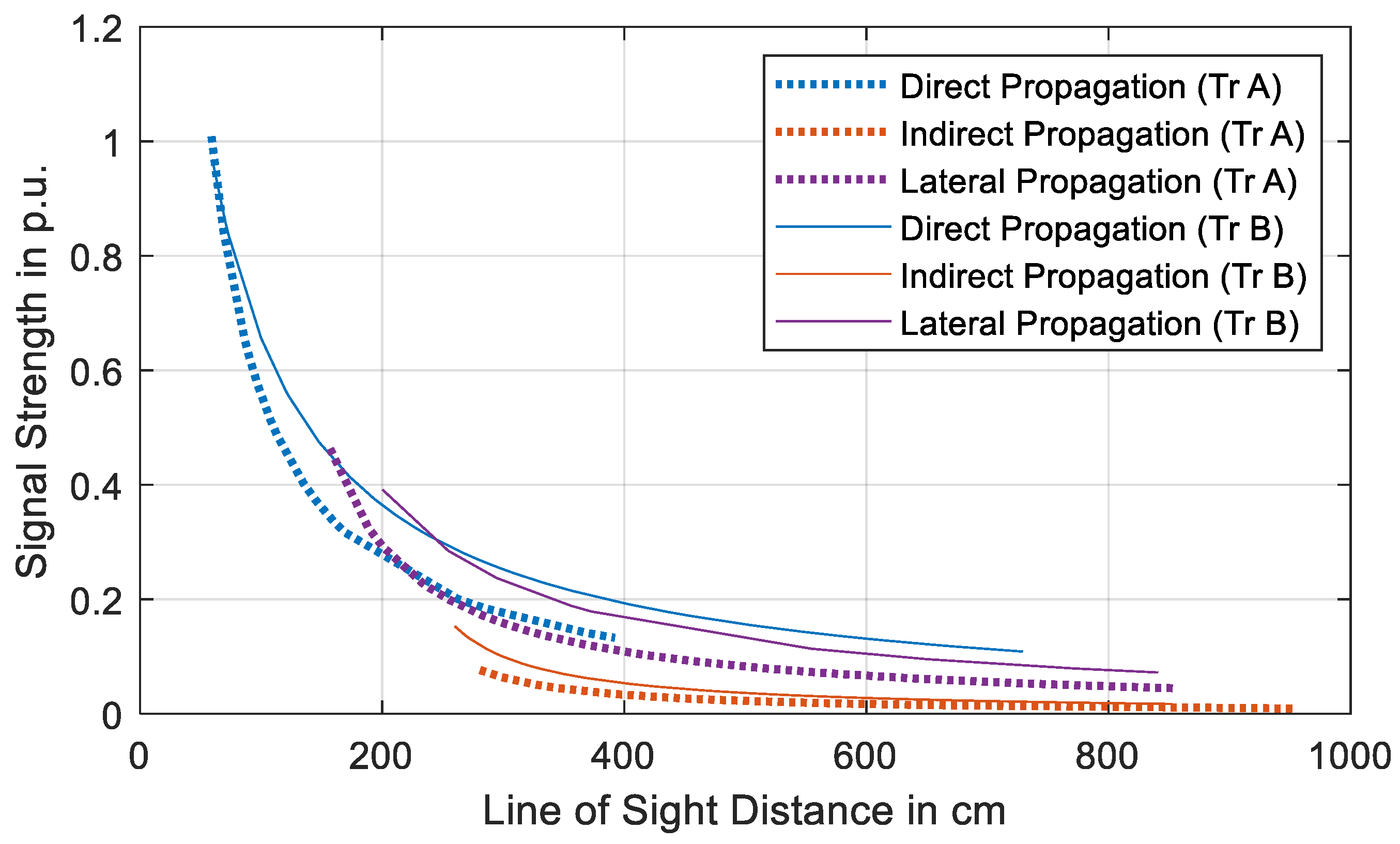
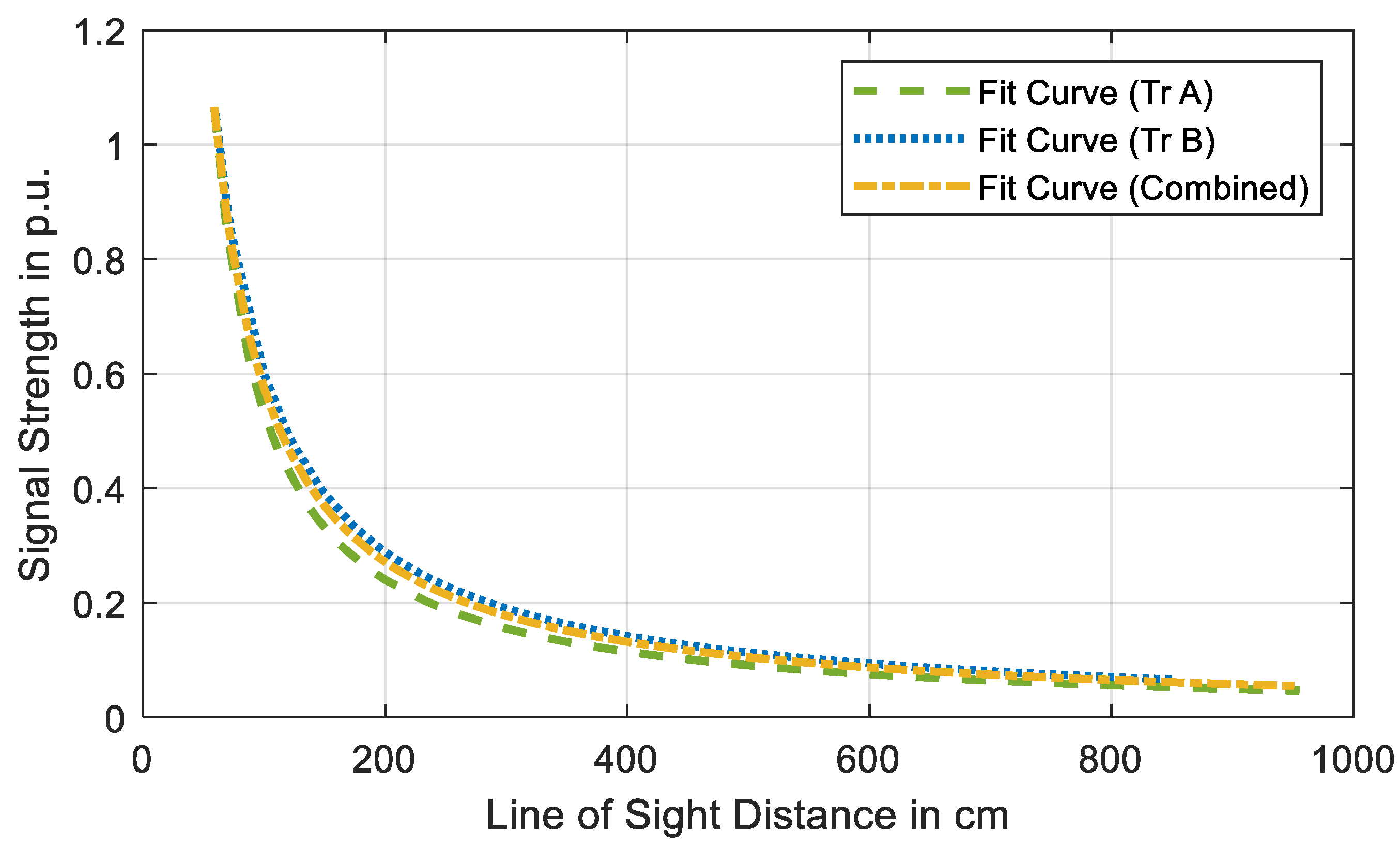
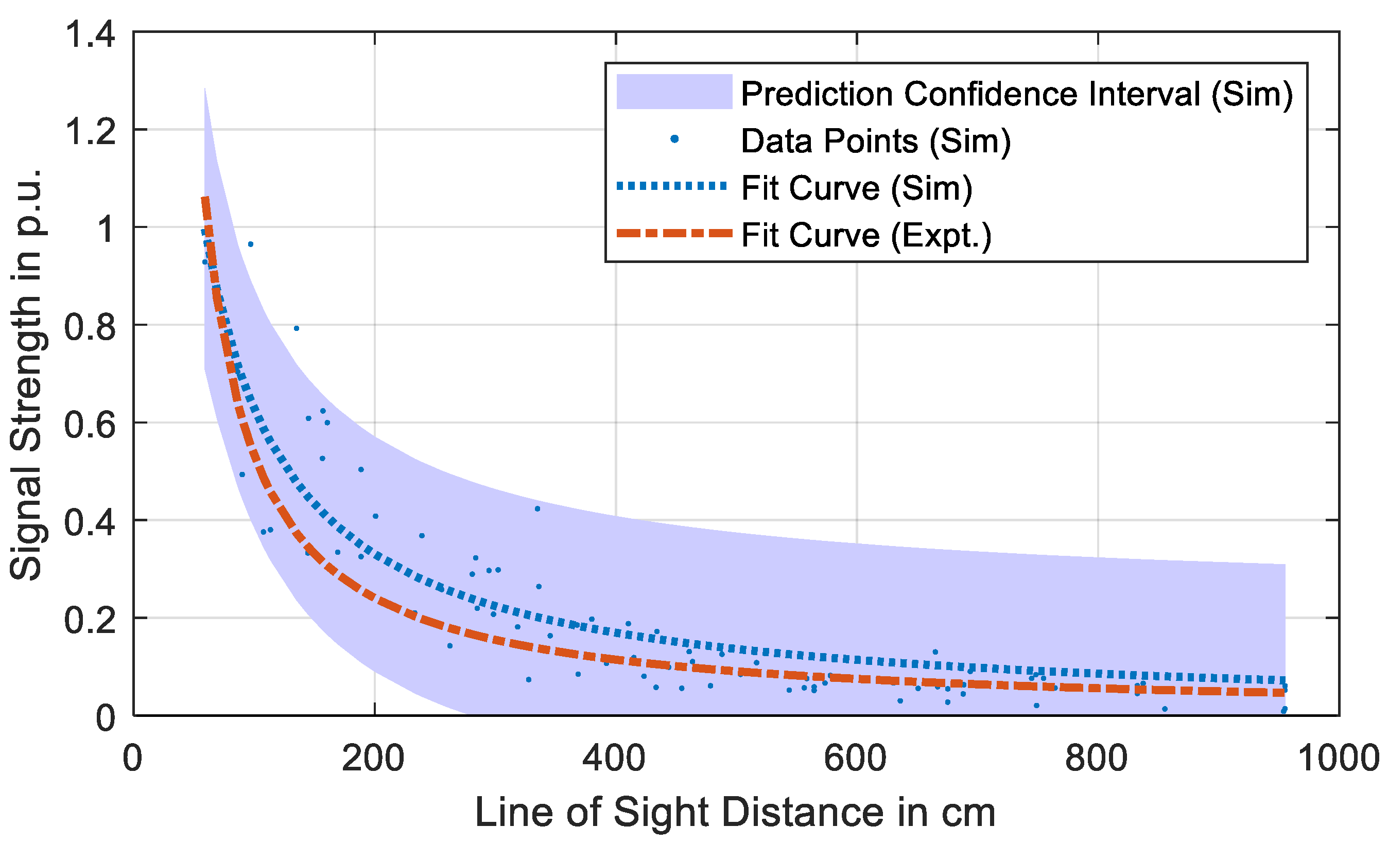
4.2. Distance-Dependent Signal Attenuation

The signal attenuation with respect to the distance between source and receiver was analyzed for both transformers. For analysis of the signal behavior, three types of propagation were defined; namely, direct, indirect, and lateral. When the source and receiver were on the same tank wall, the propagation was considered to be “direct”, as there should be minimal obstacles to signal propagation. When the source and receiver were on opposite tank walls, the signal propagation was considered to be “indirect”, as the EM waves would have to propagate around the active part. Lastly, the third category, “lateral”, was used when the source or receiver were on the side wall of the transformer.

As shown in Figure 4, there is an expected decline in signal strength with increasing distance in the case of transformer A. All signals are represented relative to the strongest measured signal. The maximum peak-to-peak voltage of the measured signals, as defined in [29], was defined as the “signal strength” and was used to compare the signals. The strongest signal was measured at a line-of-sight (LoS) distance of 69 cm between the source and the receiver, and the weakest signal was measured at an LoS distance of 650 cm. The weakest measured signal was attenuated by approximately −40.5 dB compared to the strongest measured signal, i.e., the weakest measured signal was approximately 0.9% of the strongest measured signal. Curve fitting using a hyperbolic equation was used to determine the numerical relationship between signal strength and distance since a hyperbolic equation corresponds to far field attenuation, i.e., the amplitude of the electromagnetic radiation is inversely proportional to the distance from the antenna [30]. An R² value of 0.8515 was obtained on curve fitting, which implies that 85.15% of the data points can be explained by the fit curve. As is evident from Figure 4, the signal attenuates more in the first 200 cm compared to the next 600 cm. The relationship between signal strength (y) and LoS distance (x) is found to be

$$y=\frac{43.8}{x-17.75}.$$

(1)

In comparison, the data from transformer B showed similar results to those obtained from transformer A, as shown in Figure 5. The strongest signal is measured at an LoS distance of 70 cm and the weakest signal at an LoS distance of 692 cm. Additionally, the weakest measured signal is attenuated by approximately −37 dB compared to the strongest measured signal, i.e., approximately 1.4% of the strongest measured signal. From these results, it can be observed that the attenuation in transformer A is marginally higher compared to that in transformer B. Curve fitting with a hyperbolic equation yields an R² value of 0.7709, which is a worse fit than in the case of transformer A. The obtained relationship between signal strength and LoS distance is shown in Equation (2), and a comparison of different quantitative parameters of transformers A and B is shown in

Table 1. Comparison of quantitative parameters between transformers A and B.

Parameters	Transformer A	Transformer B
Tank dimensions (cm × cm × cm)	900 × 400 × 260	900 × 400 × 260
Maximum attenuation (dB)	−40.5	−37
LoS distance at maximum attenuation (cm)	650	692
Goodness of fit (R2)	0.8515	0.7709

.

$$y=\frac{55.71}{x-7.102}$$

(2)

Next, the measurement data obtained from both transformers were separated on the basis of the three aforementioned types of signal propagation paths, as shown in Figure 6. Similar conclusions can be drawn for both transformers, namely that the signal attenuation is higher at comparable LoS distances when the propagation is indirect. Additionally, the signal attenuation is similar in the case of direct propagation and lateral propagation, indicating that lateral propagation is also direct. It should be noted that the relative orientation of the sending and receiving antennas could also have an impact on signal attenuation, particularly in indirect propagation, where the radiation pattern of the monopole could lead to increased propagation distances. However, an analysis of propagation distance is required to draw these conclusions.

Since curve fitting shows that the distance-dependent signal attenuation in both transformers can be represented as hyperbolic equations, both datasets were combined to form a unified dataset. The unified dataset was used to determine the overall distance-dependent attenuation in the two transformers. Curve fitting with a hyperbolic equation resulted in an R² value of 0.7934, which is comparable to that obtained in the case of transformer B. The obtained curve is shown in Figure 7, and the obtained equation is

$$y=\frac{51.35}{x-10.77}$$

(3)

Thus, even in the case of multiple transformers with similar ratings and different internal components, the signal attenuation characteristics remain similar.

Analysis of specific sensor positions in the case of transformer B showed that the best performing sensors are located near the outer limbs of the 5-limb core, probably because of the lack of obstructions in these regions [21]. From the standpoint of electric field intensity, these positions are away from the active part and hence encounter lower electric field stress from the 50/60 Hz operating voltage of the transformer [19]. High electric field stress from the transformer could have the unintended effect of causing PD activity in the sensor. These findings are the reason why sensors 6, 13, 22, and 23 were chosen as sources in the case of transformer A. Based on the findings from Section 4.1, since the signals remain the same when the source and receiver are interchanged (reciprocal system), these four sources can be analyzed as receivers. The distance-dependent attenuation of each receiver is shown in Figure 8 with the corresponding fit curves. All sensors have relatively similar performance. However, it can be observed that sensor 6 has the worst performance compared to the other sources, even though it is in proximity to sensors 1–9. Sensor 23, which is located near the top of the right tank wall, consistently outperforms sensor 6 at comparable LoS distances. Similar conclusions can be drawn by comparing sensors 13 and 22, where sensor 22 outperforms sensor 13 at comparable LoS distances. In conclusion, sensors installed on the side walls perform better than those installed on the front and rear tank walls. Overall, sensor 22 is the best performing sensor, receiving the highest signal strengths even at longer distances.

Frequency-domain analysis showed that, in the case of transformer A, the frequency spectrum of the signals remained similar at different LoS distances, as shown in Figure 9a, which is different from what is observed in the case of transformer B [21]. When the source is at position 6, receiver 3 is the nearest sensor on the same tank wall (59 cm), receiver 14 is the farthest sensor on the opposite tank wall (651 cm), and receiver 21 is the farthest sensor on the side wall (and the farthest sensor overall at an LoS distance of 856 cm). It can be observed that the resonant frequency spectrum of all three signals remains similar.

However, in the case of transformer B, the frequency spectrum of the signals started resembling the frequency spectrum of the noise floor at very long LoS distances [21], as shown in Figure 9b. The reason for such a difference between the two transformers is that the bushings had been removed in the case of transformer B, which allowed external frequencies to influence the frequency spectrum of the measured signals. In the case of transformer A, the bushings were still intact and prevented such interference.

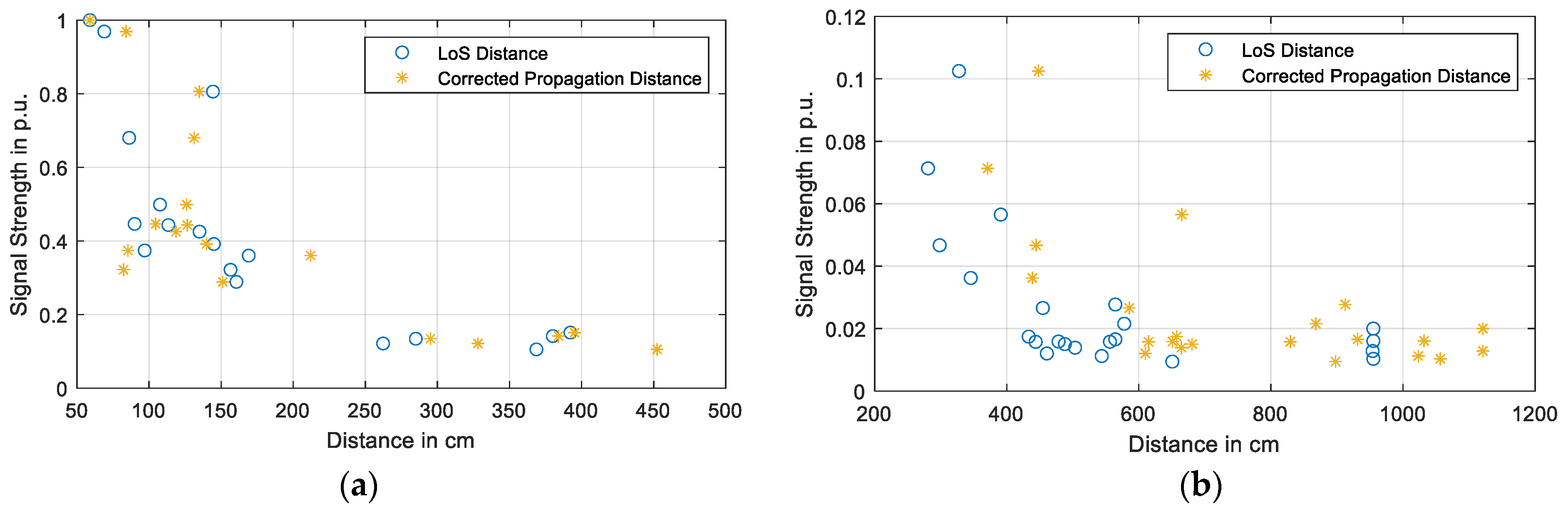
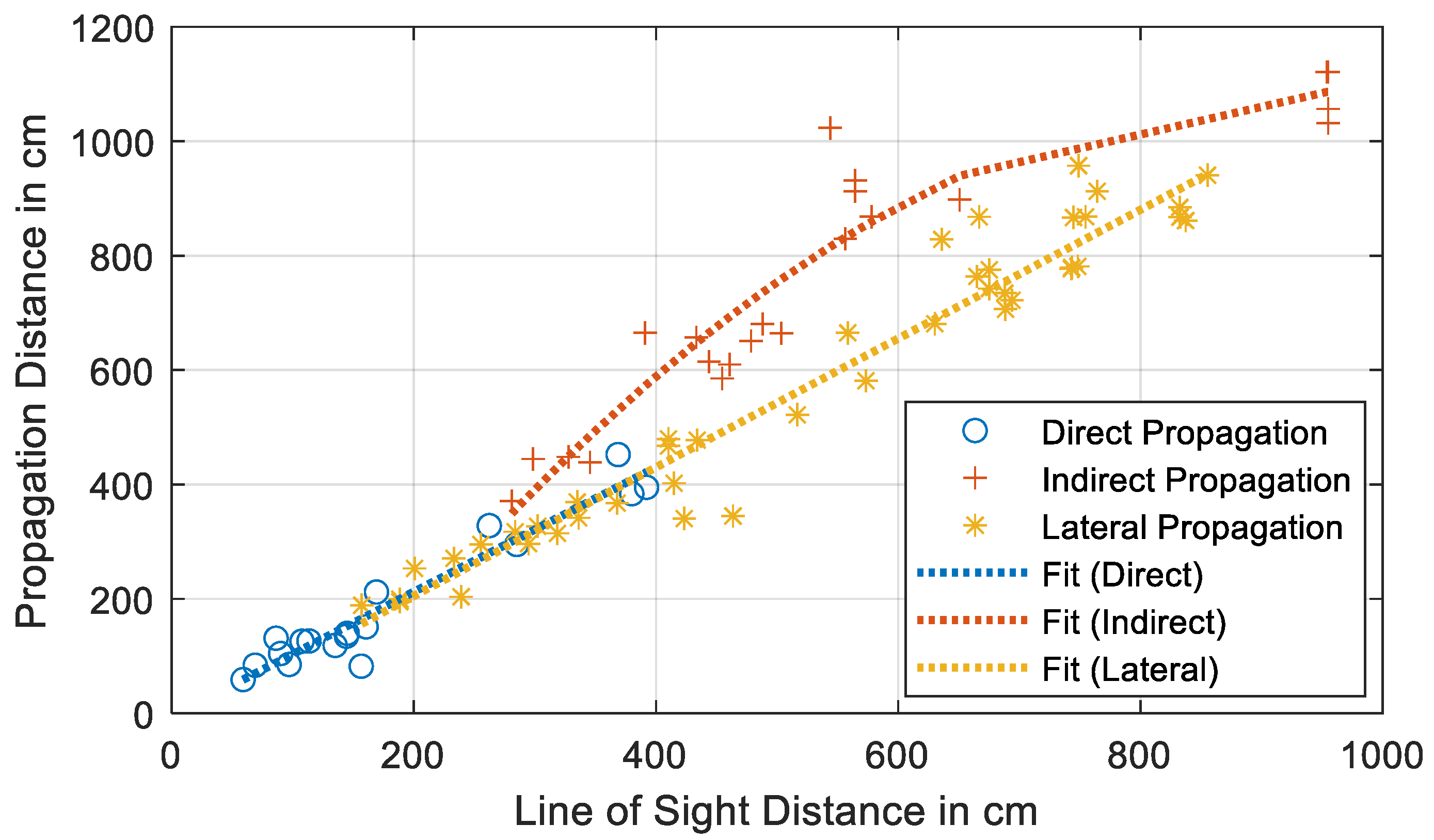
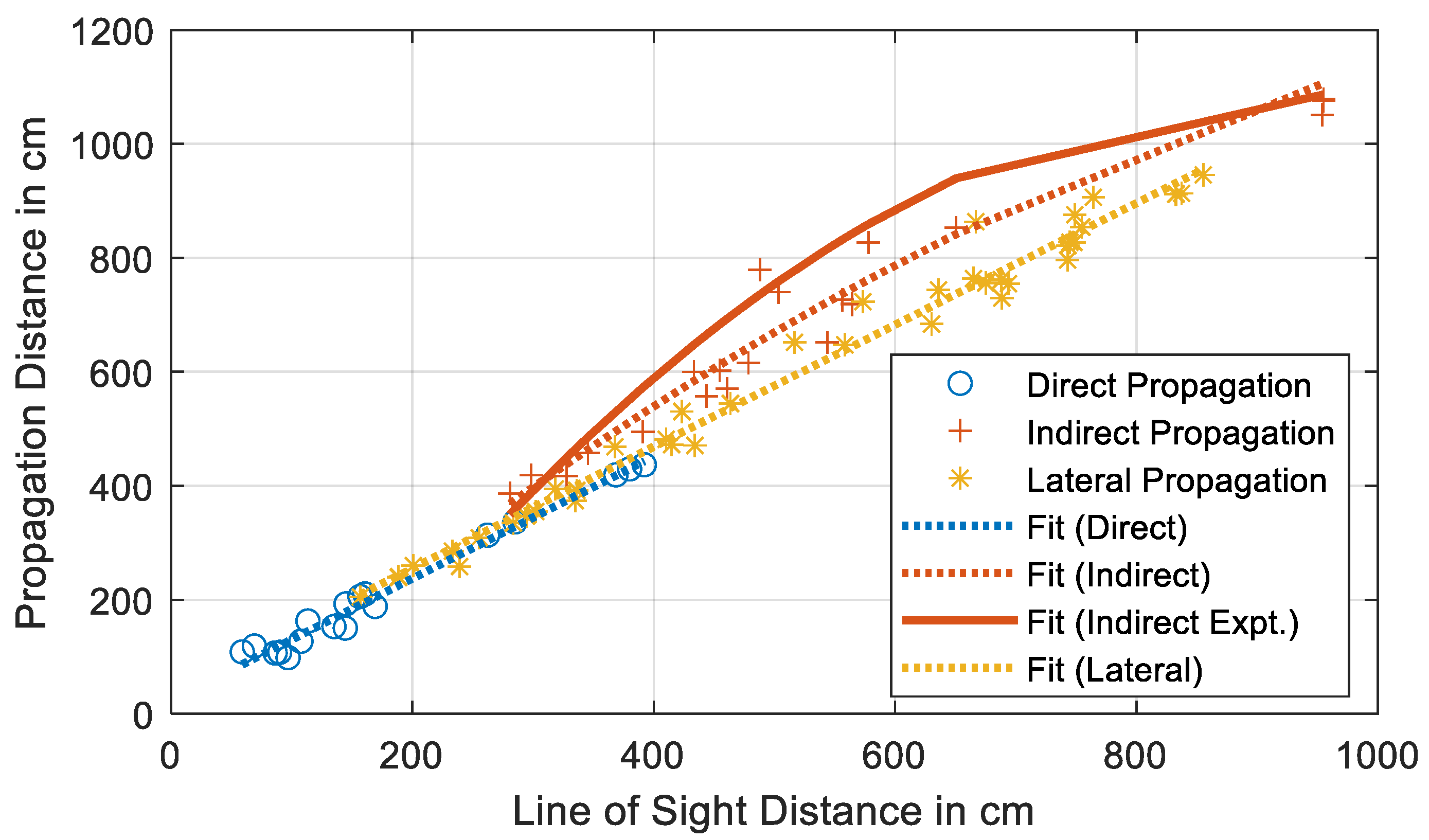
4.3. Line-of-Sight Distance vs. Propagation Distance

An important consideration in evaluating distance-dependent attenuation is whether to use LoS distance or propagation distance. As the name suggests, LoS distance is a straight line between the source and receiver, ignoring any obstacles, which is a significant simplification. However, propagation distance considers the actual path taken by the EM waves to reach the receiver and hence provides a more accurate representation of the distance-dependent signal attenuation. In this test setup, the propagation distance can be calculated using the time of arrival (ToA) of the signal at the receiver and the speed of the EM waves in the insulation medium. Since the oil was drained from the transformer tank, the insulation medium is air, and thus the EM waves travel at the speed of light. The ToA is determined by the Hinkley criterion, where the partial energy of the signal is calculated, and the instant at which the minimum value of the partial energy occurs is the ToA of the signal [29]. In this analysis, the measurement data from transformer A were used. In the case of transformer B, the ToAs could not be obtained because of the limitations of the experiment and could only be analyzed using a simulation model.

After the calculation of the propagation distance, the distance-dependent attenuation was studied and compared to that in the case of the LoS distances. A difference in the length of the measurement cables resulted in an error of approximately 3 ns in the ToAs (which equals 60 cm LoS distance). Therefore, all ToAs were corrected by adding a time delay of 3 ns. In Figure 10, the LoS distances and the corrected propagation distances of signals received from sensor 6 are shown for direct and indirect propagation. It can be observed that the difference between LoS distance and propagation distance is more pronounced in the case of indirect propagation.

The relationship between LoS distance and propagation distance is shown in Figure 11. As expected, for direct propagation, the relationship is approximately a straight line through the origin with a slope of 45°, thus indicating that the propagation distance is approximately equal to the LoS distance when propagation is direct. In the case of indirect propagation, the relationship is not linear. Instead, it is a quadratic relationship between the two distances with an R² value of 0.9006 and is given by the following equation:

y = −0.0017 x² + 3.1336 x − 400.2

(4)

The initial slope of the fit shows a rapid increase in propagation distance in comparison to LoS distance, which shows that propagation distance is longer than LoS distance. Then, the rate-of-rise decreases as the LoS distances start approaching the maximum length of the tank. However, the most interesting results are found in the case of lateral propagation, where the relationship between the two distances is similar to that observed in the case of direct propagation. These findings are comparable to those obtained from tests conducted on transformer B [21] and also from the conclusions drawn from Section 4.3. Therefore, it can be concluded that signal propagation, when the sensors are installed on the side tank walls, is direct, and thus, the signals experience lower attenuation even at longer LoS distances. It is best to place sensors at as many locations as possible, but because this is not practically feasible, positions near the sides of the transformer are recommended. Additionally, the signal propagation characteristics are similar in the case of transformers with similar power rating and tank size but different internal structures (5-limb vs. 3-limb core). Additionally, since propagation distance is calculated from ToA, the same conclusions can be drawn by analyzing the ToA instead of propagation distance.

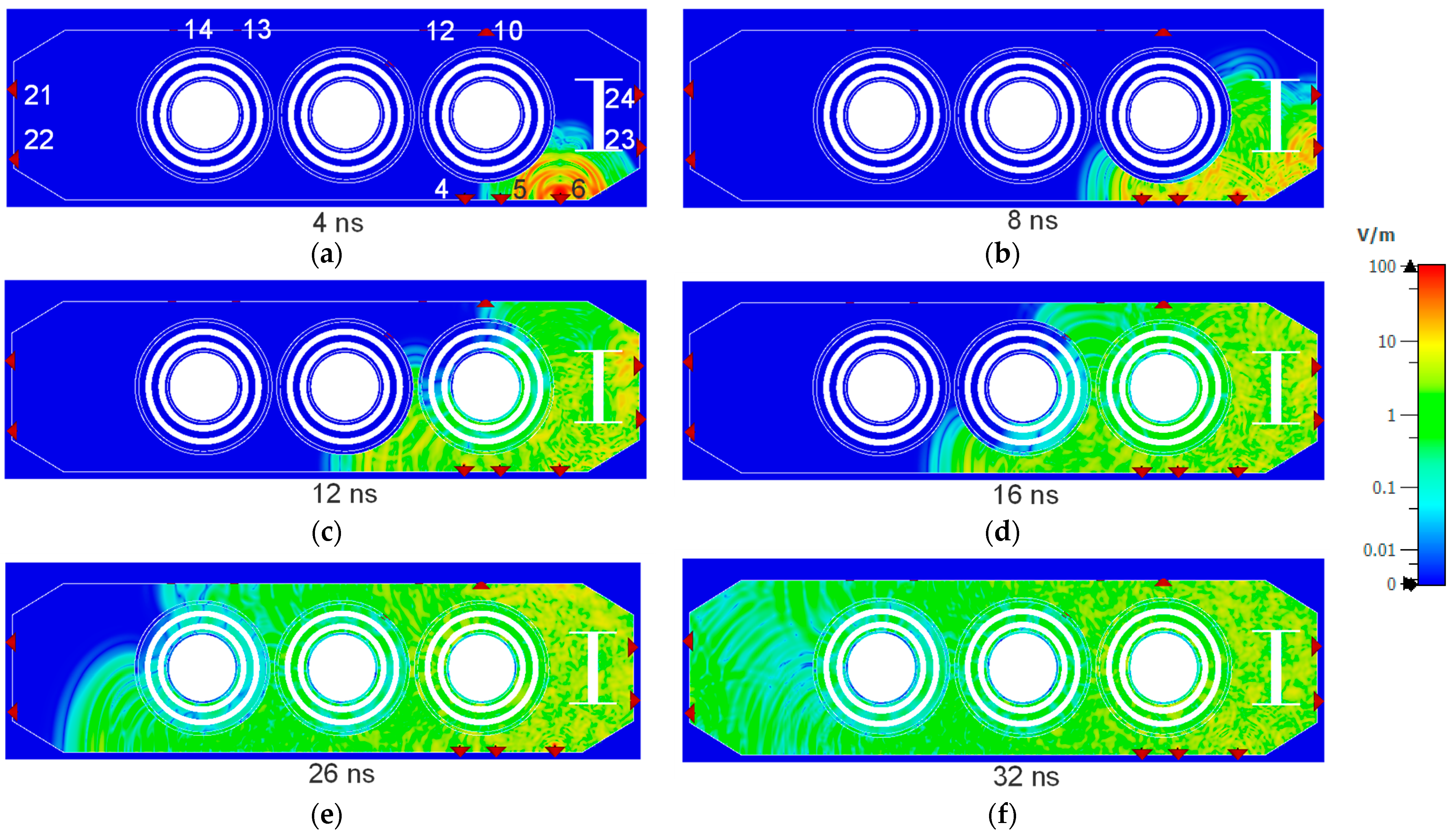
4.4. Simulation Results

For transformer A, the distance-dependent attenuation observed in the simulation results is shown and compared with the experimental results in Figure 12. It can be observed that the attenuation trend of the simulation and the experimental data is similar; however, there is an offset between the simulation and experimental results, which occurs because signal attenuation in the simulation model is lower. For example, in the case of simulation, the lowest measured peak-to-peak signal strength is 4% of the maximum measured signal, whereas, in the case of the experiment, that value is 0.9%. Curve fitting was used to analyze the overall distance-dependent attenuation for all sources, and using a hyperbolic function yielded an R² value of 0.8203, which is comparable to the experimental results. The relationship between signal strength and distance was found to be

$$y=\frac{69.74}{x+11.01}$$

(5)

The coefficients in Equation (5) reflect the offset between the simulation and experimental results (when compared with Equation (2)). However, such an offset can be easily corrected. Since a similar percentage of the data points can be explained by the hyperbolic fit curve, it can be concluded that the signal attenuation characteristics are well replicated in the simulation model. Since the deviations in signal strength depending on sensor positions are also replicated in the simulation model, it can be concluded that the deviation in signal strength is caused by the local effects of individual positions.

Next, the signal propagation was analyzed using the various propagation distances obtained from the simulation results, which were compared with those obtained from the experimental results. For this analysis, signal propagation paths were separated into three types, similar to Figure 11. It can be observed in Figure 13 that the relationship between propagation and LoS distance is approximately a straight line through the origin with a slope of 45° in the case of direct and lateral propagation, which matches the observations from the measurements. However, in the case of indirect propagation, even though the propagation distance is more than the LoS distance in the simulation results, it is apparent that the signals take a longer path in reality.

Hence, the simulation model underestimates the propagation distance in the case of indirect propagation. To improve this aspect, the simulation model would require the addition of more detail, thus leading to significantly increased simulation times. More detailed modeling of the winding would not help since the gaps between the winding discs or layer would lead to even shorter ToAs, i.e., shorter propagation distances. However, the general conclusions that can be drawn from analyzing the propagation distances are similar to those obtained from the experimental results. Therefore, the simulation model can be validated on the basis of signal attenuation and propagation characteristics with discussed restrictions.

The electromagnetic wave propagation can be visualized using the electric field strength inside the transformer tank at different times. In Figure 14, the EM wave propagation with the source at position 6 is shown at different times. The view is from the top of the tank with a cutting plane at the installation height of sensor 6. As the PD signal starts, it takes approximately 4 ns for the signal to reach the nearest sensor on the cutting plane (sensor 5). In approximately 8 ns, the EM waves have reached the sensors installed on the right side of the tank. Since the waves cannot pass through the winding or the reactor, it takes approximately 12 ns for the signal to travel around the winding and the reactor to reach the nearest sensor on the opposite side of the tank (sensor 10). It takes approximately 16 ns for the EM waves to travel across half the length of the tank. In approximately 26 ns, the signal has reached the farthest sensor on the opposite side of the tank (sensor 14). Lastly, it takes approximately 32 ns for the signals to reach the sensors installed on the left side of the tank. Therefore, in approximately 32 ns, EM waves have propagated through the entirety of the tank, which is similar to what was observed in the simulation model of transformer B, which has the same tank size. Hence, it can be concluded that in transformers with similar tank sizes but different internal components, the propagation times of the UHF signals are still comparable.

5. Conclusions

In this contribution, the results of UHF PD experiments performed on two transmission transformers were discussed and compared. The two transformers had the same specifications and tank dimensions; however, their active parts had different designs and additional internal components were at different locations. Monopoles were installed at different points on the transformer tanks. A monopole was selected as the source, and an artificial PD pulse was used to send signals, which were received by the remaining monopoles. The following aspects of the received signals were analyzed, namely the signal attenuation with respect to distance and the frequency spectra of the signals at different distances. It was observed that the distance-dependent signal attenuation characteristics were similar in the case of both transformers. A hyperbolic fit curve provided a similar fit in both cases with similar R² values, which showed that signal strength is inversely proportional to the distance from the source, i.e., far field conditions are present. In the frequency-domain, minor differences were observed in the frequency-domain results since the bushings of transformer B had been removed during the experiments. Hence, it could be concluded that the signal attenuation and propagation are similar in transformers with similar specifications and tank sizes, even though the internal design is different. This information implies that generalized signal propagation and attenuation models can be developed for one transformer and used with minor changes in other similar transformers.

Next, the signal propagation times and distances were analyzed and compared with the LoS distances using the measurement data obtained from transformer A. It was found that when signal propagation is direct or lateral, there is a linear relationship between LoS distance and propagation distance. In the case of direct propagation, the LoS distance is approximately equal to the propagation distance, and in the case of lateral propagation, the propagation distance is marginally longer than the LoS distance and can be considered to be direct propagation. However, in the case of indirect propagation, the relationship is not linear, i.e., the rate at which propagation distance increases is higher initially and starts to taper off as the LoS distances approach the length of the tank. With this information, mathematical propagation models can be developed, which would aid in the localization of PD sources.

The performance of different sensor positions was also analyzed. It was found that sensors positioned on the side tank walls of the transformers had the best performance since the signal propagation from most sources was direct. Additionally, sensors on the front and rear tank walls that were positioned near the outer limbs of the core also received signals comparable to the sensors installed on the side tank walls. These findings are consistent with previous research [19,21], thus identifying the best positions for UHF sensors to obtain strong PD signals.

Lastly, a simulation model of transformer A was built and validated on the basis of signal attenuation and propagation. The distance-dependent attenuation in the simulation model was lower than the experimental setup, which was expected because of fewer obstacles in the simulation model. However, the distance-dependent attenuation characteristics were similar to the experimental results and could be represented with a hyperbolic fit equation that was comparable to that obtained from the experimental analysis. The relationship between propagation distance and LoS distance was comparable to the experimental results as well. The linear trend during direct and lateral propagation was well replicated in the simulation model. The quadratic trend during indirect propagation was also observed. However, the slope was steeper in the experimental results, which demonstrates the impact of the additional obstacles in the measurement setup. Overall, even with simplified geometry, the simulation results showed similar characteristics as those of the measurements, and hence, the model was considered to be of sufficient quality.

6. Outlook

The validated simulation model will be used in conjunction with deep learning algorithms to investigate the possibility of accurate localization of PD sources. Additionally, the model will also be used to test the suitability of different sensor designs for PD detection.

References

1. Hussain, M.R.; Refaat, S.S.; Abu-Rub, H. Overview and Partial Discharge Analysis of Power Transformers: A Literature Review. IEEE Access 2021, 9, 64587–64605. [Google Scholar] [CrossRef]
2. Dukanac, D. Application of UHF method for partial discharge source location in power transformers. IEEE Trans. Dielectr. Electr. Insul. 2018, 25, 2266–2278. [Google Scholar] [CrossRef]
3. Judd, M.D.; Yang, L.; Hunter, I. Partial discharge monitoring of power transformers using UHF sensors. Part I: Sensors and signal interpretation. IEEE Electr. Insul. Mag. 2005, 21, 5–14. [Google Scholar] [CrossRef]
4. Jahangir, H.; Akbari, A.; Azirani, M.A.; Werle, P.; Szczechowski, J. Turret-Electrode Antenna for UHF PD Measurement in Power Transformers—Part I: Introduction and Design. IEEE Trans. Dielectr. Electr. Insul. 2020, 27, 2113–2121. [Google Scholar] [CrossRef]
5. Chai, H.; Phung, B.T.; Zhang, D. Development of UHF Sensors for Partial Discharge Detection in Power Transformer. In Proceedings of the 2018 Condition Monitoring and Diagnosis (CMD), Perth, WA, USA, 23–26 September 2018; IEEE: Piscataway, NJ, USA, 2018; pp. 1–5, ISBN 978-1-5386-4126-2. [Google Scholar]
6. Cruz, J.d.N.; Serres, A.J.R.; de Oliveira, A.C.; Xavier, G.V.R.; de Albuquerque, C.C.R.; da Costa, E.G.; Freire, R.C.S. Bio-inspired Printed Monopole Antenna Applied to Partial Discharge Detection. Sensors 2019, 19, 628. [Google Scholar] [CrossRef] [PubMed] [Green Version]
7. Zhou, X.; Wu, X.; Ding, P.; Li, X.; He, N.; Zhang, G.; Zhang, X. Research on Transformer Partial Discharge UHF Pattern Recognition Based on Cnn-lstm. Energies 2020, 13, 61. [Google Scholar] [CrossRef] [Green Version]
8. Do, T.-D.; Tuyet-Doan, V.-N.; Cho, Y.-S.; Sun, J.-H.; Kim, Y.-H. Convolutional-Neural-Network-Based Partial Discharge Diagnosis for Power Transformer Using UHF Sensor. IEEE Access 2020, 8, 207377–207388. [Google Scholar] [CrossRef]
9. Xue, N.; Yang, J.; Shen, D.; Xu, P.; Yang, K.; Zhuo, Z.; Zhang, L.; Zhang, J. The Location of Partial Discharge Sources Inside Power Transformers Based on TDOA Database with UHF Sensors. IEEE Access 2019, 7, 146732–146744. [Google Scholar] [CrossRef]
10. Nobrega, L.; Costa, E.; Serres, A.; Xavier, G.; Aquino, M. UHF Partial Discharge Location in Power Transformers via Solution of the Maxwell Equations in a Computational Environment. Sensors 2019, 19, 3435. [Google Scholar] [CrossRef] [PubMed] [Green Version]
11. Mirzaei, H.; Akbari, A.; Gockenbach, E.; Miralikhani, K. Advancing new techniques for UHF PDdetection and localization in the power transformers in the factory tests. IEEE Trans. Dielectr. Electr. Insul. 2015, 22, 448–455. [Google Scholar] [CrossRef]
12. Siegel, M.; Coenen, S.; Beltle, M.; Tenbohlen, S.; Weber, M.; Fehlmann, P.; Hoek, S.M.; Kempf, U.; Schwarz, R.; Linn, T.; et al. Calibration Proposal for UHF Partial Discharge Measurements at Power Transformers. Energies 2019, 12, 3058. [Google Scholar] [CrossRef] [Green Version]
13. Jahangir, H.; Akbari, A.; Werle, P.; Szczechowski, J. Possibility of PD calibration on power transformers using UHF probes. IEEE Trans. Dielectr. Electr. Insul. 2017, 24, 2968–2976. [Google Scholar] [CrossRef]
14. Mirzaei, H.R.; Akbari, A.; Zanjani, M.; Miralikhani, K.; Gockenbach, E.; Borsi, H. Investigating suitable positions in power transformers for installing UHF antennas for partial discharge localization. In Proceedings of the International Conference on Condition Monitoring and Diagnosis (CMD), Bali, Indonesia, 23–27 September 2012; IEEE: Piscataway, NJ, USA, 2012; pp. 625–628, ISBN 978-1-4673-1020-8. [Google Scholar]
15. Coenen, S.; Tenbohlen, S. Location of PD sources in power transformers by UHF and acoustic measurements. IEEE Trans. Dielect. Electr. Insul. 2012, 19, 1934–1940. [Google Scholar] [CrossRef]
16. Ishak, A.M.; Judd, M.D.; Siew, W.H. A study of UHF partial discharge signal propagation in power transformers using FDTD modelling. In Proceedings of the 45th International Universities’ Power Engineering Conference, UPEC 2010, Cardiff, UK, 31 August–3 September 2010; Institution of Engineering and Technology: London, UK, 2011; pp. 1–5, ISBN 978-1-4244-7667-1. [Google Scholar]
17. Nobrega, L.A.; Xavier, G.V.; Serres, A.J. Investigating reflections and refractions effects in the UHF Location of partial discharges in power transformers using time domain simulation. In Proceedings of the 2018 Simposio Brasileiro de Sistemas Eletricos (SBSE), Niteroi, Brazil, 12–16 May 2018. [Google Scholar]
18. Du, J.; Chen, W.; Cui, L.; Zhang, Z.; Tenbohlen, S. Investigation on the propagation characteristics of PD-induced electromagnetic waves in an actual 110 kV power transformer and its simulation results. IEEE Trans. Dielect. Electr. Insul. 2018, 25, 1941–1948. [Google Scholar] [CrossRef]
19. Beura, C.P.; Beltle, M.; Tenbohlen, S.; Siegel, M. Quantitative Analysis of the Sensitivity of UHF Sensor Positions on a 420 kV Power Transformer Based on Electromagnetic Simulation. Energies 2020, 13, 3. [Google Scholar] [CrossRef] [Green Version]
20. BSS Hochspannungstechnik GmbH. HFIG-600 VHF/UHF High Power Impulse Generator. Available online: https://www.bss-hochspannungstechnik.de/pdf/Datasheet%20HFIG-600.pdf (accessed on 20 February 2022).
21. Beura, C.P.; Beltle, M.; Tenbohlen, S. Positioning of UHF PD Sensors on Power Transformers Based on the Attenuation of UHF Signals. IEEE Trans. Power Deliv. 2019, 34, 1520–1529. [Google Scholar] [CrossRef]
22. Tenbohlen, S.; Coenen, S.; Siegel, M.; Linn, T.; Markalous, S.; Mraz, P.; Beltle, M.; Naderian, A.; Schmidt, V.; Fuhr, J.; et al. Improvements to PD measurements for factory and site acceptance tests of power transformers. In Cigre Technical Brochure 861; Cigre: Paris, France, 2022. [Google Scholar]
23. Beura, C.P.; Beltle, M.; Tenbohlen, S. Attenuation of UHF Signals in a 420 kV Power Transformer Based on Experiments and Simulation. In Proceedings of the 21st International Symposium on High Voltage Engineering, Budapest, Hungary, 26–30 August 2019; Németh, B., Ed.; Springer International Publishing: Cham, Switzerland, 2020; pp. 1276–1285, ISBN 978-3-030-31679-2. [Google Scholar]
24. Zanjani, M.; Akbari, A.; Mirzaei, H.R.; Shirdel, N.; Gockenbach, E.; Borsi, H. Investigating partial discharge UHF electromagnetic waves propagation in transformers using FDTD technique and 3D simulation. In Proceedings of the IEEE International Conference on Condition Monitoring and Diagnosis (CMD 2012), Bali, Indonesia, 23–27 September 2012; IEEE: Piscataway, NJ, USA, 2012; pp. 497–500, ISBN 978-1-4673-1019-2. [Google Scholar]
25. Yang, L.; Judd, M.D.; Costa, G. Simulating propagation of UHF signals for PD monitoring in transformers using the finite difference time domain technique. In Proceedings of the 17th Annual Meeting of the IEEE Lasers and Electro-Optics Society, LEOS 2004, Boulder, CO, USA, 17–20 October 2004; IEEE: Piscataway, NJ, USA, 2004; pp. 410–413, ISBN 0-7803-8584-5. [Google Scholar]
26. Giglia, G.; Ala, G.; Castiglia, V.; Imburgia, A.; Miceli, R.; Rizzo, G.; Romano, P.; Schettino, G.; Viola, F. Electromagnetic Full-Wave Simulation of Partial Discharge Detection in High Voltage AC Cables. In Proceedings of the 2019 IEEE 5th International forum on Research and Technology for Society and Industry (RTSI), Florence, Italy, 9–12 September 2019; IEEE: Piscataway, NJ, USA, 2019; pp. 166–171, ISBN 978-1-7281-3815-2. [Google Scholar]
27. Akbarzadeh, A.R.; Shen, Z. On the Gap Source Model for Monopole Antennas. IEEE Antennas Wirel. Propag. Lett. 2008, 7, 115–118. [Google Scholar] [CrossRef]
28. Umemoto, T.; Tenbohlen, S. Novel Simulation Technique of Electromagnetic Wave Propagation in the Ultra High Frequency Range within Power Transformers. Sensors 2018, 18, 4236. [Google Scholar] [CrossRef] [PubMed] [Green Version]
29. Beura, C.P.; Beltle, M.; Tenbohlen, S. Study of the Influence of Winding and Sensor Design on Ultra-High Frequency Partial Discharge Signals in Power Transformers. Sensors 2020, 20, 5113. [Google Scholar] [CrossRef] [PubMed]
30. Balanis, C.A. Modern Antenna Handbook; Wiley-Blackwell: Oxford, UK, 2008; ISBN 978-0-470-03634-1. [Google Scholar]
Figure 1. Positions of sensors on the different tank walls of transformer A: (a) front view; (b) left side view; (c) rear view; (d) right side view.
Energies 15 02766 g001
Figure 2. Artificial PD pulse in the (a) time-domain; (b) frequency-domain (FFT).
Energies 15 02766 g002
Figure 3. Reciprocity test of signals when the source and receiver are reversed: (a) time-domain; (b) frequency-domain.
Energies 15 02766 g003
Figure 4. Signal attenuation in transformer A with the corresponding fit curve.
Energies 15 02766 g004
Figure 5. (a) Signal attenuation in transformer B with the corresponding fit curve; (b) comparison of fit curves of transformers A and B.
Energies 15 02766 g005
Figure 6. Comparison of signal propagation paths in transformers A and B.
Energies 15 02766 g006
Figure 7. Comparison of the fit curves of transformers A, B, and the combined dataset.
Energies 15 02766 g007
Figure 8. Comparison of attenuation of signals received from the individual sources.
Energies 15 02766 g008
Figure 9. Comparison of the frequency spectra of signals received from receivers at varying LoS distances for (a) transformer A; (b) transformer B.
Energies 15 02766 g009
Figure 10. Correction of the propagation distance for signals received from sensor 6: (a) direct propagation; (b) indirect propagation.
Energies 15 02766 g010
Figure 11. Relationship between propagation distance and LoS distance.
Energies 15 02766 g011
Figure 12. Signal attenuation in the simulation model of transformer A with corresponding fit curve and comparison with the fit curve obtained from experimental data.
Energies 15 02766 g012
Figure 13. Relationship between propagation distance and LoS distance in the simulation model.
Energies 15 02766 g013
Figure 14. Electromagnetic wave propagation at different times when the PD source is at position 6 (transformer A): (a) at 4 ns; (b) at 8 ns; (c) at 12 ns; (d) at 16 ns; (e) at 26 ns; (f) at 32 ns.
Energies 15 02766 g014