Numerical Simultaneous Determination of Non-Uniform Soot Temperature and Volume Fraction from Visible Flame Images

Abstract

This paper presents a method to invert the two-dimensional distribution of a temperature and volume concentration of soot particles from color images. By using numerical simulation, the temperature field and particle volume-concentration field of a non-uniform soot flame are simultaneously reconstructed using the wide-response spectrum of a color CCD camera without adding monochromatic filters. The influence of number of cameras, error of camera position angle, measurement noise and different reconstruction algorithms on measurement accuracy are analyzed. The numerical-simulation results demonstrate that camera-position angle errors play a crucial role in the reconstruction accuracy. In addition, increasing the number of cameras can improve the reconstruction result accuracy. Compared with the least squares algorithm, the Tikhonov-regularization algorithm has a stronger anti-noise ability and can resist 39 dB of noise. The conclusions obtained in this paper are helpful to guide following experimental studies.

1. Introduction

Flame temperature is one of the most important combustion parameters [1,2]. Accurate temperature measurement is of great significance for improving combustion efficiency and reducing pollutant emissions [3]. Thermocouple temperature measurement is one of the most common temperature-measurement methods, which has the advantages of simple operation and reliable results. However, it is a contact measurement method, and it is easy to interfere with a measured flame-flow field when the method is used for flame measurement, thereby affecting the temperature-field distribution of the flame [4,5]. Non-contact measurement will not interfere with the measured flame-flow field, and it has certain advantages in flame-temperature measurement. Laser spectroscopy is one of the non-contact temperature-measurement methods, which include laser interference holography [6,7,8], tunable semiconductor-laser absorption spectroscopy (TDLAS) technology [9,10,11,12] and laser Rayleigh scattering (LRS) technology [13,14,15,16]. In recent years, the measurement of the temperature fields of a flame section has been performed by combining TDLAS and CT technologies [11,17,18]. Laser spectral-temperature-measurement technology has the advantages of a high measurement accuracy and large measurement range when measuring a flame’s temperature. However, the temperature-measurement process requires the help of lasers. In addition, corresponding optical paths are arranged, and the operation process has a certain complexity. It is challenging to use laser spectroscopy for temperature measurement in some high-vibration and high-dust industrial environments [19,20,21].

Compared with laser spectroscopy technology, temperature-measurement technology based on spontaneous flame-radiation information is another type of non-contact passive temperature-measurement method, which does not require a laser light source [22]. During the combustion process of fuel, a large amount of heat is released due to a chemical reaction; the heat is externally manifested as a thermal-radiation spectrum. When measuring flame temperature based on flame-excitation radiation information, it is necessary to use a sensor to collect thermal-radiation information. An image sensor is commonly used [23]. As the most common industrial camera, the CCD camera is widely used in temperature measurement due to its advantages [24,25,26]. This method has the advantages of not affecting the measured flame-flow field, and it performs without an external light source. All flame-flow field information can be collected by a CCD camera, and several algorithms can be used to reconstruct the flame-flow field parameters [27,28].

The algorithm used to reconstruct a flame-flow field based on a CCD camera consists of inverting the radiation source term of the flame-flow field from the boundary radiation intensity collected by the CCD camera. The process of inversion has a high computational load and is time-consuming. In addition, it is prone to errors due to the fact that an ill-posed problem is considered. At present, it is mainly divided into two categories: optimization algorithms [29,30,31,32] and regularization algorithms [33,34,35,36]. Liu et al. [29] transformed the inversion problem into an optimization problem. They used the conjugate gradient method to obtain a boundary radiation intensity with the smallest error from experimental data. Wang et al. [30] transformed the inversion problem into an ill-conditioned matrix. They used the least-squares QR-decomposition algorithm to solve the optimal radiation source term and then obtained the parameters of a flame-flow field from the optimal radiation source term. Although the least-squares QR-decomposition algorithm used by Wang et al. is analytically equivalent to the conjugate-gradient algorithm used by Liu et al., the least-squares QR-decomposition algorithm is more advantageous in terms of the processing of numerical properties. The optimization algorithm is well developed and is widely used to solve such inversion problems. However, the optimization algorithm is an iterative algorithm that requires one to set a suitable convergence range. An inappropriate convergence range will lead to large errors and a long calculation time. Zhou et al. [37] proposed an improved Tikhonov-regularization algorithm for the reconstruction of a three-dimensional temperature field. The obtained error of the experimental results was almost 5%. Wei et al. [38] improved the overall accuracy of reconstruction using the Tikhonov-regularization algorithm. They efficiently reduced the number of projection angles that are required for reconstruction. Xie et al. [39] used both the Tikhonov-regularization algorithm and the truncated singular-value algorithm in order to reconstruct a flame in a furnace. The experimental results demonstrated that the former algorithm takes less time, its reconstruction error is small and its maximum temperature reconstruction is more accurate. Previous studies showed that the Tikhonov-regularization algorithm can accurately reproduce the distribution of different parameters of the flame-flow field and has great potential.

In addition, in previous studies, the wavelengths of the three channels of the CCD camera were often approximated by using the monochromatic wavelength in order to calculate radiation intensity [40,41,42,43,44]. However, the spectral response of the $R$, $G$ and $B$ bands of the color CCD camera is relatively wide and cannot be simply approximated by using the monochromatic wavelength. Yan et al. [45] considered the broad spectrum of the color CCD camera when inverting axisymmetric flames. The experimental results showed that this method is efficient and reliable.

Based on the previous studies, this study used a color CCD camera to collect flame images, reconstruct the two-dimensional temperature field and radiation characteristics of the flame by using the Tikhonov-regularization algorithm and perform a verification of the numerical simulation of the bimodal flame. This paper is divided into the following three steps: establishing a numerical simulation of a double-peak flame, calculating the image intensity collected by the camera according to the spectral-band model and using the Rayleigh approximation formula to calculate the spectral-absorption coefficient. The calculated image intensity is used to reconstruct the temperature-field distribution of the flame section by using the Tikhonov-regularization algorithm. Finally, the reconstruction results are compared with those obtained using the LSQR algorithm.

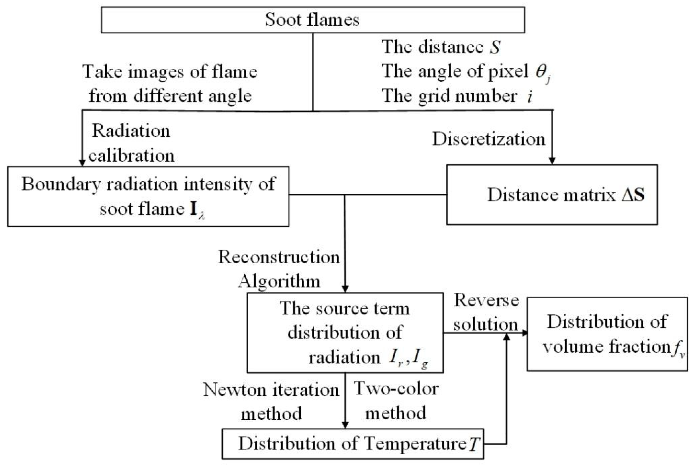
2. Reconstruction Principle

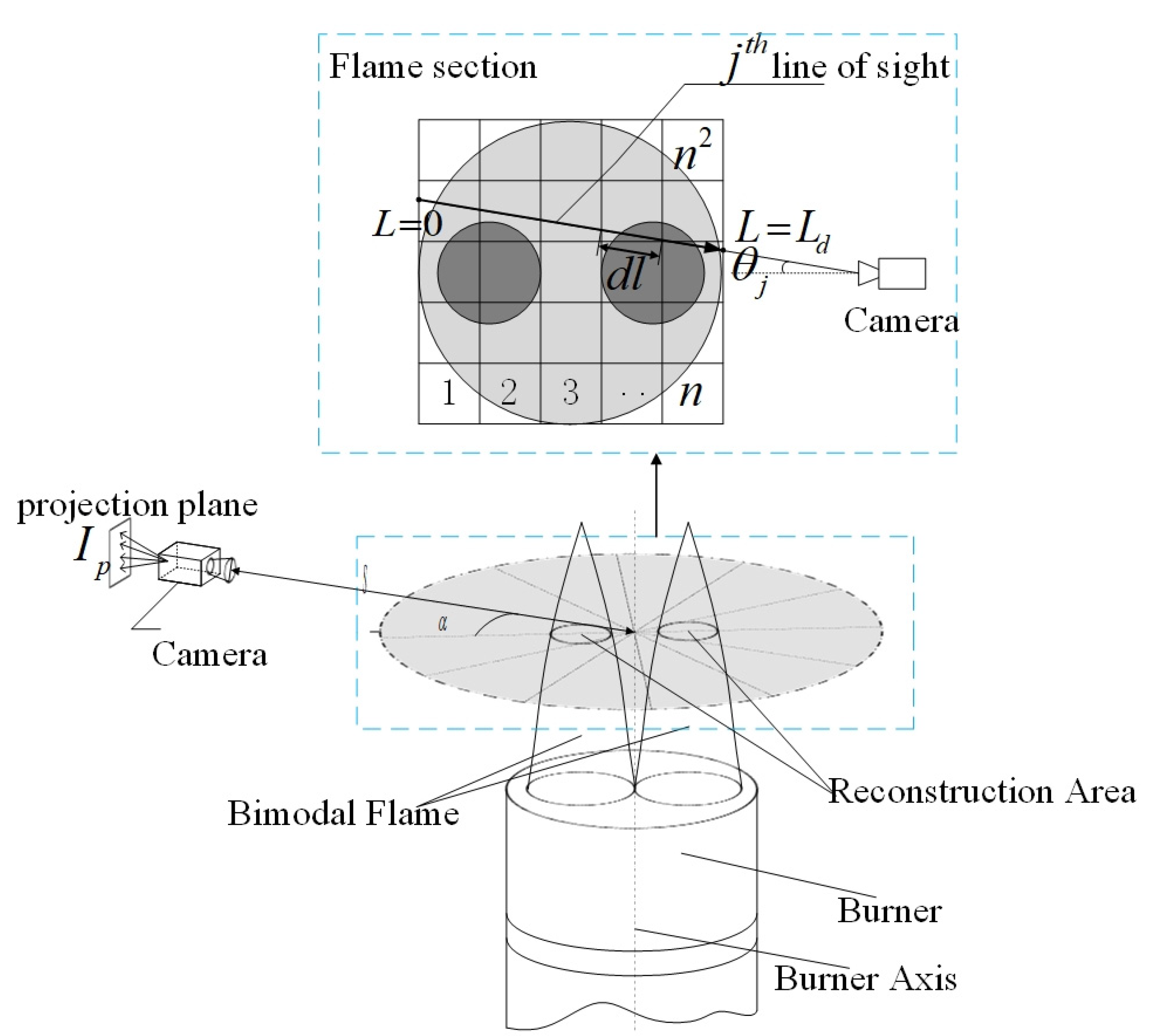
2.1. Radiation Imaging Models

The tomographic reconstruction of asymmetric flames usually requires multiple angles to provide a complete distribution of information on the flame. If images of flames are used for reconstruction, multiple cameras are required. To this end, this paper proposes a flame cross-section radiation-parameter reconstruction system, which is specially designed to perform a multi-camera tomographic reconstruction of the flame, as shown in Figure 1. Multiple cameras are placed at the same angle, $\alpha$, and same distance, $S$, from the flame axis. The flame images are then simultaneously collected. The pixel intensity of the flame image is processed in order to obtain the radiation source-term distribution of the flame cross-section. The soot-temperature distribution and volume fraction are then calculated by using colorimetry, as described in the next section.

2.2. Direct Problem

For hydrocarbon-fuel combustion flames, the radiation of ${\mathrm{CO}}_2$ and ${\mathrm{H}}_2\mathrm{O}$ in the visible light band is negligible, while the radiation of the flame in the visible light band is mainly generated by soot at high temperature [46]. In general, the flame radiation intensity is described by the Radiation Transfer Equation (RTE) [40]. In this paper, the following assumptions are made [35,36,47,48,49]: (a) only the soot radiation in the visible light band is considered, (b) the effects of scattering and self-absorption of the flame are ignored and (c) the effect of background-light radiation is ignored.

According to these assumptions, the radiation intensity of soot along the projection path received by the camera can be expressed as:

$$I_{\lambda }={\displaystyle {\int }_0^{L_d}\kappa \left(L,\lambda \right)I_b}\left(L,\lambda ,T\right)\mathrm{d}l$$

(1)

where $\lambda$ is the wavelength, $L$ represents the projected path length, $I_b\left(L,\lambda ,T\right)$ denotes the blackbody radiation intensity of soot particles and $\kappa \left(L,\lambda \right)$ is the local spectral absorption coefficient, which is proportional to the soot-volume fraction and calculated by using the Rayleigh limit of Mie theory as [45,48]:

$${\kappa }_a=6\pi E\left(m\right)f_v/\lambda$$

(2)

where $E\left(m\right)$ is the soot optical constant and $m$ is the gradient index function with real and imaginary parts [50].

Note that $E\left(m\right)$ is related to the physical properties of soot. In this study, the most widely used function model in the literature is considered. More precisely, $E\left(m\right)=0.26,m=1.57-0.56i$.

According to Planck’s radiation law, the radiation intensity of soot particles can be expressed as:

$$I_b\left(L,\lambda ,T\right)=\frac{C_1{\lambda }^{-5}}{e^{C_2/\lambda T\left(L\right)}-1}\frac{1}{\pi }$$

(3)

where $T\left(L\right)$ represents the temperature and $C_1,C_2$ are the first and second Planck’s radiation constants, respectively [43].

In previous studies, when computing the radiation intensity of soot particles, the $R$, $G$ and $B$ data of the pixels of a flame picture collected by color CCD camera are usually assumed to be proportional to the approximately monochromatic radiative intensities in wavelengths of red, green and blue [40,41,42,43]. However, due to the wide spectral-response spectrum of the $R$, $G$ and $B$ channels of the color camera, it cannot be simply approximated by using the monochromatic radiation intensity. Assuming that the relative spectral response efficiencies of the $R$, $G$ and $B$ channels of the CCD camera are expressed as ${\eta }_R\left(\lambda \right),{\eta }_G\left(\lambda \right),{\eta }_B\left(\lambda \right)$, the projection received by the camera can be expressed as:

$$\begin{array}{l}{I}_{\lambda }={\displaystyle {\int }_0^{L_d}{\displaystyle {\int }_{{\lambda }_1}^{{\lambda }_2}{\eta }_k\left(\lambda \right)\kappa \left(\lambda \right)I_b\left(\lambda ,T\right)\mathrm{d}\lambda \mathrm{d}l}}\\ k=R,G,B\end{array}$$

(4)

where ${\lambda }_1,{\lambda }_2$ are the start and end of the corresponding wavelength of the camera, respectively.

As shown in Figure 1, the flame cross-section and camera beam are respectively discretized into $n^2$ unit grids and $p$ imaging sight lines, where the flame-radiation parameters in the unit grids are uniform. Therefore, Equation (3) can be written in a discrete form:

$$\begin{array}{l}{I}_{\lambda }\left(j\right)={\displaystyle \sum _{i=1}^{n^2}{\displaystyle {\int }_{{\lambda }_1}^{{\lambda }_2}{\eta }_k\left(\lambda \right)\kappa \left(i,\lambda \right)I_b\left(i,\lambda ,T\right)\mathrm{d}\lambda \Delta L_{j,i}}} \mathrm{or} I_{\lambda }\left(j\right)={\displaystyle \sum _{i=1}^{n^2}I\left(i,\lambda ,T\right)\Delta L_{j,i}}\\ j=1,\dots ,p \end{array}$$

(5)

where $I_b\left(i,\lambda ,T\right)$ is the radiation source term of the cell grid number $i$, ${\eta }_k\left(\lambda \right)$ represents the relative spectral-response efficiencies, $\kappa \left(i,\lambda \right)$ denotes the local spectral absorption coefficient of grid number $j$ and $\Delta L_{j,i}$ is the distance traveled by the imaging sight-line number $j$ within the grid number $i$.

Equation (5) is then written in matrix form:

$$I_{\lambda }=\Delta S\cdot I$$

(6)

where $\Delta S\in R^{P\times n^2}$, $I_{\lambda }\in R^p$ and $I\in R^{n^2}$.

It can be seen from Figure 1 that each imaging line of sight will pass through only few cell grids. Therefore, matrix $\Delta S$ is a large sparse matrix, and an ill-posed matrix-solution algorithm is required to invert reasonable results. For the inversion algorithm of large-sparse matrices, the commonly used methods are the Tikhonov-regularization algorithm and the least-squares (LSQR) algorithm based on QR decomposition. In this paper, these two algorithms are used to simultaneously reconstruct the radiation parameters of the flame section, and the influence of different measurement errors on the accuracies of the two reconstruction algorithms is evaluated.

2.3. Inverse Problem

2.3.1. LSQR Algorithm

The LSQR algorithm is suitable for solving the least-squares problem ${‖b-Ax‖}^2$, where $A$ is a large sparse matrix [40].

Equation (6) can be obtained using the LSQR algorithm:

$$\Delta S\cdot I=I_{\lambda }\to \min {‖\Delta S\cdot I-I_{\lambda }‖}^2\mathrm{or} Ax=b\to \min {‖Ax-b‖}^2$$

(7)

where $A=\Delta S$, $x=I$ and $b=I_{\lambda }$.

For the kth iterative process:

$$\begin{array}{l}{x}_k=v_k{y}_k,y_k\in R^k\\ r_k=b-A{x}_k=U_{k+1}\left({\mathsf{\beta }}_1{e}_1\right)-A{V}_k{y}_k\end{array}$$

(8)

where

$$\begin{array}{l}{U}_{k+1}=\left[u_1,u_2,\dots ,u_{k+1}\right]\\ V_k=\left[v_1,v_2,\dots ,v_k\right]\\ B_k=\left[\begin{array}{lllll}{\alpha }_1\hfill & 0\hfill & \cdots \hfill & \cdots \hfill & 0\hfill \\ {\beta }_2\hfill & {\alpha }_2\hfill & \ddots \hfill & \cdots \hfill & 0\hfill \\ ⋮\hfill & {\beta }_3\hfill & \ddots \hfill & \ddots \hfill & ⋮\hfill \\ ⋮\hfill & ⋮\hfill & \ddots \hfill & \ddots \hfill & ⋮\hfill \\ 0\hfill & \cdots \hfill & \cdots \hfill & \cdots \hfill & {\beta }_{k+1}\hfill \end{array}\right]\end{array}$$

(9)

and where $U_{k+1}$ and $V_k$ are obtained by using matrix bi-diagonalization:

$$\begin{array}{l}{\beta }_1={‖b‖}^2,u_1=b/{\beta }_1,{\alpha }_1{v}_1=A^{\mathrm{T}}{u}_1\\ U_{k+1}\left({\beta }_1{e}_1\right)=b,A{V}_k=Y_{k+1}{B}_k\\ A^{\mathrm{T}}{U}_{k+1}=V_k{B}^T{}_k+{\alpha }_{k+1}{v}_{k+1}{e}_{k+1}^{\mathrm{T}}\end{array}$$

(10)

The calculation result can be computed as:

$$\min {‖r_k‖}^2=\min {‖{\beta }_1{e}_1-B_k{y}_k‖}^2$$

(11)

2.3.2. Tikhonov-Regularization Algorithm

The Tikhonov-regularization algorithm [35] can transform the solving of Equation (6) into the solving of the minimum of the following expression:

$$R\left(I,\alpha \right)={‖I_{\lambda }-\Delta S\cdot I‖}^2+\alpha ‖D\cdot I‖$$

(12)

where $D$ is a regularized matrix for which the diagonal elements are all 1.0 and the sum of all the elements in each row is 0 [34].

An approximate solution for the regularization coefficient $\alpha$ is given by [43]:

$$\alpha \left(I_{\lambda }\right)\approx 2{‖I_{\lambda }-\Delta S\cdot I\left(0\right)‖}^2/{‖D\cdot I\left(0\right)‖}^2$$

(13)

where $I\left(0\right)$ is the least-squares solution of Equation (6).

The optimal solution of Equation (6) is then expressed as:

$$I={\left(\Delta S^{\mathrm{T}}\Delta S+\alpha D^{\mathrm{T}}D\right)}^{-1}\Delta S^{\mathrm{T}}{I}_{\lambda }$$

(14)

2.3.3. Two-Color Method

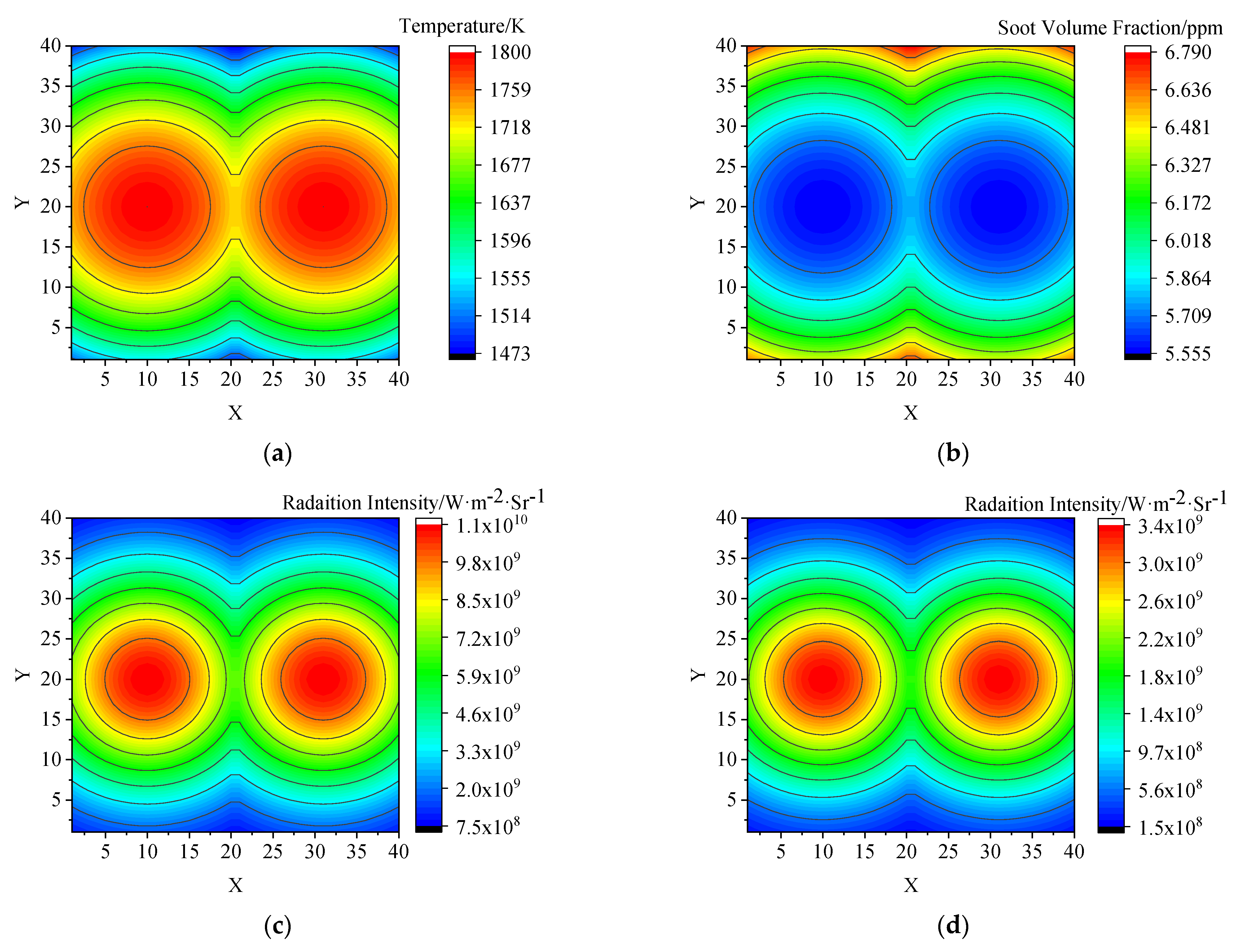
After solving the radiation source-term distribution of the flame section, the temperature distribution can be solved using the two-color method:

$$\frac{I_r}{I_g}=\frac{{\displaystyle {\int }_{{\lambda }_1}^{{\lambda }_2}{\eta }_r\left(\lambda \right){\kappa }_r\left(\lambda \right)I_{b,r}\mathrm{d}\lambda }}{{\displaystyle {\int }_{{\lambda }_1}^{{\lambda }_2}{\eta }_g\left(\lambda \right){\kappa }_g\left(\lambda \right)I_{b,g}\mathrm{d}\lambda }}$$

(15)

where $I_r$ and $I_r$ are the source-term distributions of radiation for the $R$ and $G$ channels, respectively.

Since Equation (15) comprises the integral of wavelength $\lambda$, it cannot be simply solved. Therefore, this paper develops Equation (16) about temperature $T$ and uses the Newton iteration method to solve the temperature distribution:

$$F\left(T\right)=I_r{\displaystyle {\int }_{{\lambda }_1}^{{\lambda }_2}{\eta }_g\left(\lambda \right){\kappa }_g\left(\lambda \right)I_{b,g}\left(T\right)\mathrm{d}\lambda }-I_g{\displaystyle {\int }_{{\lambda }_1}^{{\lambda }_2}{\eta }_r\left(\lambda \right){\kappa }_r\left(\lambda \right)I_{b,r}\left(T\right)\mathrm{d}\lambda }$$

(16)

After the temperature distribution is solved, the soot-concentration distribution can be reversely solved by bringing the temperature distribution into Equation (3). The overall calculation process is presented in Figure 2.

3. Simulated Object

The impacts of different errors on the reconstruction accuracy of the two algorithms are compared using a numerical simulation. The asymmetric temperature and soot-concentration distributions are expressed in Equation (17). In this system, the cameras are assumed to have a field of view of 11.4 degrees and the distance $S$ is 169 mm. The common area that the cameras can capture is a circle with a diameter of 33.78 mm in the central area. Therefore, the flame cross-section is divided into 1600 sub-units, and each sub-unit is a square with a side length of 0.6 mm in space.

$$\begin{array}{l}T\left(x,y\right)=1800e^{-\left(\frac{x^2+y^2}{2500}\right)}\\ f_v\left(x,y\right)=\frac{1}{T\left(x,y\right)}\end{array}$$

(17)

where $-19\le x\le 20$, $-19\le y\le 20$, $T\left(x,y\right)$ and $f_v\left(x,y\right)$ are, respectively, the temperature and soot-concentration distributions, as shown in Figure 3.

In this paper, the Gaussian function is used to approximate the relative spectral-response efficiency, a function of the simulated CCD camera [45,51,52]:

$$\begin{array}{l}{\eta }_i\left(\lambda \right)=C_i\exp \left[-{(\lambda -a_i)}^2/4000\right]\\ i=R,G\end{array}$$

(18)

where $C_i$ is the maximum relative spectral-response efficiency, $a_i$ is the central wavelength and ${\lambda }_1,{\lambda }_2$ are the start and end of the corresponding wavelength of the camera, respectively.

It is assumed that $C_G=1$, $C_R=0.8$, $a_R=600$ and $a_G=500$. The relative spectral-response efficiency curves of the $R$ and $G$ channels are shown in Figure 4.

For the actual flame, only the flame image collected by the CCD camera is required as the projection data in order to invert the radiation parameters of the flame section. However, for the numerical simulation, mathematical methods should be used to calculate the theoretical radiation intensity collected by CCD cameras at different angles. In this paper, in the multi-camera reconstruction system of flame-section radiation-parameter construction, three cases of camera-placement interval angles exist: $\alpha =30°$, $\alpha =60°$ and $\alpha =90°$, corresponding to 12, 6 and 4 cameras, respectively. The theoretical radiation-intensity distribution collected by the CCD camera is shown in Figure 5. The theoretical radiation intensity is calculated as described in Section 2.2.

In this paper, root mean square error (RMSE) is used to test the accuracy of the reconstructed field with the known original intensity field:

$$E=100\times \frac{\sqrt{\frac{1}{N}{\displaystyle \sum {\left(f\left(x,y\right)-f\left(x,y\right){}^{\prime }\right)}^2}}}{f_{\max }}$$

(19)

where $f\left(x,y\right)$ is the reconstructed field, $f\left(x,y\right){}^{\prime }$ represents the original intensity field, $f_{\max }$ denotes the maximum value of the original intensity field and $N$ is the number of cell grids equal to 1600 as previously mentioned.

4. Results and Discussion

4.1. Influence of the Number of Cameras

As previously mentioned, three cases for the number of cameras exist: four cameras separated by 90°, six cameras separated by 60° and twelve cameras separated by 30°. The distributions of the flame cross-section temperature reconstructed by using the two algorithms are shown in Figure 6, while the reconstructed soot concentrations are shown in Figure 7. The root mean square errors of the reconstruction results for the two algorithms with different numbers of cameras are shown in Figure 8.

It can be seen from Figure 6 and Figure 7 that when the number of CCD cameras increases, the reconstruction effects of the two algorithms are more accurate. Due to the fact that the two algorithms are equations for large sparse matrices, as the number of CCD cameras increases, more projection data can be provided, and therefore, the inversion results are better. Since the horizontal fields of view of the cameras are smaller than the separation angles of the cameras, the line of sight passing between the cameras is decreased, which results in the cameras being more prone to distortion at the boundary. The reconstruction of the soot-concentration distribution is more prone to distortion than the reconstruction of the temperature distribution. The regularization algorithm outperforms the least-squares algorithm for both the temperature and soot-concentration reconstructions. When the number of CCD cameras is more than six, the two algorithms can reconstruct a better temperature distribution. However, for the soot-concentration reconstruction, only the regularization algorithm can obtain better results.

It can be observed from Figure 8 that as the camera interval angle decreases and the number of cameras increases, the reconstruction accuracies of the two algorithms are greatly improved. The temperature-reconstruction error of the regularization algorithm decreases from 1.63% for four cameras to 0.0027% for twelve cameras. In addition, the reconstruction effect of the soot concentration is more easily affected by the number of CCD cameras. The soot-concentration reconstruction error of the four-camera regularization algorithm reaches 9.11%, while the error of the LSQR algorithm also reaches 39.8%. When the number of CCD cameras increases to 12, the error also decreases to the same level as the temperature reconstruction. Therefore, the error of the regularization algorithm is 0.0885% and that of the LSQR algorithm is 1.30%.

4.2. Effect of Measurement Noise

When a camera is used to collect flame images, it is inevitable that external light sources, the attenuation of flame light and other factors will affect the collected flame images, which affects the reconstruction accuracy. It can be seen from Figure 6 and Figure 7 that the two algorithms can accurately reconstruct the distribution of temperature and soot concentration. Therefore, in the case of limited noise, the two algorithms should also be able to more accurately reconstruct the radiation parameters of the flame section. In order to analyze the anti-noise ability of the two algorithms, a random noise (cf. Equation (20)) is added to the previously described theoretical radiation intensity. In order to avoid the reconstruction error caused by the lack of flame information collected by using the camera and the two-color method, the influence of noise on the two algorithms is analyzed using the reconstruction results of the radiation source terms of 12 cameras.

$${I^{\prime }}_{\lambda }=I_{\lambda }\left(1+\frac{R_{12}-6}{\sigma }\right)$$

(20)

where ${I^{\prime }}_{\lambda }$ and $I_{\lambda }$, respectively, represent the theoretical radiation intensity after adding noise and without adding noise, and $R_{12}$ is the sum of 12 random numbers between zero and one, representing different noise levels.

In this paper, signal-to-noise ratio (SNR) is used to evaluate the noise intensity. The SNR is calculated (in dB) using Equation (21). In the calculation process, four different noise levels are considered: $\sigma =50$, $\sigma =800$, $\sigma =900$ and $\sigma =2200$. The corresponding SNRs are: 39 dB, 63 dB, 65 dB and 72 dB, respectively. The theoretical radiation intensity with added noise is shown in Figure 9, and the reconstruction-error results are shown in Figure 10.

$$SNR=20\lg \left(\frac{{I^{\prime }}_{\lambda }}{{I^{\prime }}_{\lambda }-I_{\lambda }}\right)$$

(21)

It can be seen from Figure 10 that as the noise level decreases, the reconstruction effect of the two algorithms gradually becomes better. A comparison of the two algorithms shows that the regularization algorithm introduces the regularization matrix $D$ and the regularization coefficient $\alpha$ based on the LSQR algorithm and obtains the final result by using the inversion of the ill-posed matrix. Therefore, the regularization algorithm has a stronger anti-noise ability than the LSQR algorithm. Although the SNR reaches 39 dB, the reconstruction error of the regularization algorithm is only almost 4%. In addition, the regularization algorithm can still accurately reconstruct the radiation source-term distribution. The anti-noise ability of the LSQR algorithm is far less than that of the regularization algorithm. Only when the SNR is reduced to 63 dB can the LSQR algorithm have a reconstruction error of almost 10%. However, it is still higher than the regularization algorithm by almost 4%.

Moreover, the time consumed by the reconstruction process is also important to the evaluation of the algorithm. Figure 11 represents the time consumed by the two algorithms under different noise levels. It can be seen that the regularization algorithm takes a slightly longer time than the LSQR algorithm. This is due to the fact that the LSQR algorithm is the basis of the regularization algorithm, both of which are required to iterate the matrix, and the regularization algorithm is required to further regularize the iterative results of the LSQR algorithm, which results in a longer time needed by the regularization algorithm. In general, as the number of elements of the coefficient matrix increases, the iteration time required by the LSQR algorithm sharply increases, which results in an increase in the algorithm time. However, increasing the number of cells in the reconstructed source term will increase the reconstruction accuracy. Therefore, it is necessary to make a trade-off between the reconstruction time and reconstruction accuracy in order to achieve an efficient balance between them.

4.3. Error of Camera-Separation Angle

As previously mentioned, the camera separation angles (30°, 60° and 90°) are the same. However, in the actual experiment, the angles between the cameras would inevitably have an angle deviation due to the experimental equipment, reading errors and other reasons. In order to analyze the influence of the angle deviation on the reconstruction accuracy of the two algorithms, different degrees of angle error were added to the acquisition angles of the 12 cameras and the radiation source term was reconstructed accordingly. The obtained results are shown in Figure 12.

It can be seen from Figure 12 that four angular errors of 0.1°, 0.3°, 1° and 3° are added to the acquisition angle. The radiation source terms of the $R$ and $G$ channel reconstructions of the two algorithms are highly affected by the interval-angle error. In addition, the RMS rapidly increases with the increase of the angle error. When the angle error is 2°, the RMS of the regularization algorithm exceeds 30%, and the reconstruction results at this time can no longer be used to reconstruct the radiation parameters of the flame section. The impact of the LSQR algorithm is far greater than that of the regularization algorithm. More precisely, when the angle error is 0.1°, the reconstruction error of the LSQR algorithm exceeds 60%. It can be deduced from this analysis that camera acquisition angle is highly important for the two algorithms, and it is the basis for determining whether the inversion can be achieved. By analyzing the generation principle of the theoretical images, the reason why the angle error has a high influence can be determined. In fact, the flame image is a “cumulative effect” formed by a specific radiation-source item, a specific acquisition angle, a specific line of sight and a specific grid. The deviation of the angle when collecting the flame image will cause the flame images provided by multiple cameras to be contradictory, which leads to inversion errors. In contrast to the effects of the number of cameras and noise on the previously detailed two algorithms, the camera acquisition angle affects the inversion process, while its impact on the two algorithms is extremely significant.

5. Conclusions

This paper proposes a method to simultaneously reconstruct the two-dimensional temperature field and soot-particle volume concentration of a non-uniform soot flame using the wide response spectrum of a color CCD camera. It then evaluates the influence of number of cameras, camera interval-angle error and noise on the Tikhonov-regularization algorithm and LSQR algorithm. The numerical-simulation results demonstrate that when the number of cameras increases, the reconstruction accuracy of the two algorithms increases. The Tikhonov-regularization algorithm has a higher precision than the LSQR algorithm. When six cameras are used, the error of reconstructed RMS of the Tikhonov-regularization algorithm’s temperature and soot-volume concentration are 0.0259% and 0.5522%, respectively. In contrast, those of the LSQR algorithm are 0.3497% and 3.6418%, respectively. Furthermore, the Tikhonov-regularization algorithm outperforms the LSQR algorithm in terms of noise immunity. If the LSQR algorithm requires a satisfactory accuracy, the SNR of the flame images should not be less than 65 dB. However, for the Tikhonov-regularization algorithm, the SNR of the images needs to be better than only 39 dB, which is much better than that of the LSQR algorithm. Most importantly, the camera separation-angle error has a high impact on the reconstruction accuracy. Finally, an angle error of 1° will bring an almost 18% error to the Tikhonov-regularization algorithm and a more than 100% error to the LSQR algorithm.

References

1. Lee, T.; Bessler, W.G.; Kronemayer, H.; Schulz, C.; Jeffries, J.B. Quantitative temperature measurements in high-pressure flames with multiline NO-LIF thermometry. Appl. Opt. 2005, 44, 6718–6728. [Google Scholar] [CrossRef]
2. Chen, H.Y.; Hou, Y.Q.; Wang, X.; Pan, Z.X.; Xu, H.M. Characterization of In-Cylinder Combustion Temperature Based on a Flame-Image Processing Technique. Energies 2019, 12, 2386. [Google Scholar] [CrossRef] [Green Version]
3. Li, W.H.; Lou, C.; Sun, Y.P.; Zhou, H.C. Estimation of radiative properties and temperature distributions in coal-fired boiler furnaces by a portable image processing system. Exp. Therm. Fluid Sci. 2011, 35, 416–421. [Google Scholar] [CrossRef]
4. Loboda, E.L.; Reino, V.V.; Agafontsev, M.V. Choice of a spectral range for measuring temperature fields in a flame and recording high-temperature objects screened by the flame using ir diagnostic methods. Russ. Phys. J. 2015, 58, 278–282. [Google Scholar] [CrossRef]
5. Salinas, C.T.; Pu, Y.; Lou, C.; dos Santos, D.B. Experiments for combustion temperature measurements in a sugarcane bagasse large-scale boiler furnace. App. Therm. Eng. 2020, 175, 115433. [Google Scholar] [CrossRef]
6. Xiao, X.D.; Choi, C.W.; Puri, I.K. Temperature measurements in steady two-dimensional partially premixed flames using laser interferometric holography. Combust. Flame 2000, 120, 318–332. [Google Scholar] [CrossRef]
7. Doi, J.; Sato, S. Three-dimensional modeling of the instantaneous temperature distribution in a turbulent flame using a multidirectional interferometer. Opt. Eng. 2007, 46, 015601. [Google Scholar]
8. Wang, D.Z.; Zhuang, T.G. The measurement of 3-D asymmetric temperature field by using real time laser interferometric tomography. Opt. Lasers Eng. 2001, 36, 289–297. [Google Scholar] [CrossRef]
9. Chen, H.; Du, Y.; Ding, Y.; Peng, Z. Non-uniform temperature measurement of flat flames using TDLAS. In Fourth Seminar on Novel Optoelectronic Detection Technology and Application; Guofan, J., Guangjun, Z., Eds.; International Society for Optics and Photonics: Bellingham, WA, USA, 2018; Volume 10697. [Google Scholar]
10. Cui, H.; Wang, F.; Huang, Q.; Yan, J.; Cen, K. Multiparameter Measurement in Ethylene Diffusion Flame Based on Time-Division Multiplexed Tunable Diode Laser Absorption Spectroscopy. IEEE Photonics J. 2019, 11, 1–12. [Google Scholar] [CrossRef]
11. Wang, Z.; Zhou, W.; Kamimoto, T.; Deguchi, Y.; Yan, J.; Yao, S.; Girase, K.; Jeon, M.-G.; Kidoguchi, Y.; Nada, Y. Two-Dimensional Temperature Measurement in a High-Temperature and High-Pressure Combustor Using Computed Tomography Tunable Diode Laser Absorption Spectroscopy (CT-TDLAS) with a Wide-Scanning Laser at 1335–1375 nm. App. Spectrosc. 2020, 74, 210–222. [Google Scholar] [CrossRef]
12. Most, D.; Leipertz, A. Simultaneous two-dimensional flow velocity and gas temperature measurements by use of a combined particle image velocimetry and filtered Rayleigh scattering technique. Appl. Opt. 2001, 40, 5379–5387. [Google Scholar] [CrossRef] [PubMed]
13. Hoffman, D.; Munch, K.U.; Leipertz, A. Two-dimensional temperature determination in sooting flames by filtered Rayleigh scattering. Opt. Lett. 1996, 21, 525–527. [Google Scholar] [CrossRef] [PubMed]
14. Feng, D.; Goldberg, B.M.; Shneider, M.N.; Miles, R.B. Optimization of Filtered Rayleigh Scattering for the Measurement of Pressure and Temperature. Combust. Sci. Technol. 2020, 1–19. [Google Scholar] [CrossRef]
15. Bookey, H.T.; Bishop, A.I.; Barker, P.F. Narrow-band coherent Rayleigh scattering in a flame. Opt. Express 2006, 14, 3461–3466. [Google Scholar] [CrossRef]
16. Kampmann, S.; Leipertz, A.; Dobbeling, K.; Haumann, J.; Sattelmayer, T. Two-dimensional temperature measurements in a technical combustor with laser Rayleigh scattering. Appl. Opt. 1993, 32, 6167–6172. [Google Scholar] [CrossRef]
17. Ma, L.; Li, X.; Sanders, S.T.; Caswell, A.W.; Roy, S.; Plemmons, D.H.; Gord, J.R. 50-kHz-rate 2D imaging of temperature and H2O concentration at the exhaust plane of a J85 engine using hyperspectral tomography. Opt. Express 2013, 21, 1152–1162. [Google Scholar] [CrossRef] [Green Version]
18. Liu, C.; Cao, Z.; Lin, Y.; Xu, L.; McCann, H. Online Cross-Sectional Monitoring of a Swirling Flame Using TDLAS Tomography. IEEE Trans. Instrum. Meas. 2018, 67, 1338–1348. [Google Scholar] [CrossRef] [Green Version]
19. Liu, X.D.; Hao, X.J.; Xue, B.; Tai, B.; Zhou, H.C. Two-Dimensional Flame Temperature and Emissivity Distribution Measurement Based on Element Doping and Energy Spectrum Analysis. IEEE Access 2020, 8, 200863–200874. [Google Scholar] [CrossRef]
20. Zapka, W.; Pokrowsky, P.; Tam, A.C. Noncontact optoacoustic monitoring of flame temperature profiles. Opt. Lett. 1982, 7, 477–479. [Google Scholar] [CrossRef]
21. Liu, D.; Yan, J.H.; Wang, F.; Huang, Q.X.; Chi, Y.; Cen, K.F. Simultaneous experimental reconstruction of three-dimensional flame soot temperature and volume fraction distributions. Acta Phys. Sin. 2011, 60, 6. [Google Scholar]
22. Liu, G.N.; Liu, D. Inverse radiation analysis for simultaneous reconstruction of temperature and volume fraction fields of soot and metal-oxide nanoparticles in a nanofluid fuel sooting flame. Int. J. Heat Mass Transf. 2018, 118, 1080–1089. [Google Scholar] [CrossRef]
23. Liu, D.; Huang, Q.X.; Wang, F.; Chi, Y.; Cen, K.F.; Yan, J.H. Simultaneous Measurement of Three-Dimensional Soot Temperature and Volume Fraction Fields in Axisymmetric or Asymmetric Small Unconfined Flames With CCD Cameras. J. Heat Transf. Trans. ASME 2010, 132, 061202. [Google Scholar] [CrossRef]
24. Jiang, F.; Liu, S.; Liangi, S.Q.; Li, Z.H.; Wang, X.Y.; Lu, G. Visual Flame Monitoring System Based on Two-Color Method. J. Therm. Sci. 2009, 18, 284–288. [Google Scholar] [CrossRef]
25. Li, Z.H.; Liu, S.; Mu, H.P.; Jiang, F.; Guo, J.M. Calibration and Experimental Research of a Multiple-wavelength Flame Temperature Instrumentation System. J. Therm. Sci. 2004, 13, 371–375. [Google Scholar] [CrossRef]
26. Huang, Y.; Yan, Y. Transient two-dimensional temperature measurement of open flames by dual-spectral image analysis. Trans. Inst. Meas. Control. 2000, 22, 371–384. [Google Scholar] [CrossRef]
27. Huang, Q.X.; Liu, D.; Wang, F.; Yan, J.H.; Chi, Y.; Cen, K.F. Study on three-dimensional flame temperature distribution reconstruction based on truncated singular value decomposition. Acta Phys. Sin. 2007, 56, 6742–6748. [Google Scholar] [CrossRef]
28. Liu, D.; Wang, F.; Cen, K.F.; Yan, J.H.; Huang, Q.X.; Chi, Y. Noncontact temperature measurement by means of CCD cameras in a participating medium. Opt. Lett. 2008, 33, 422–424. [Google Scholar] [CrossRef]
29. Liu, L.H.; Tan, H.P. Inverse radiation problem in three-dimensional complicated geometric systems with opaque boundaries. J. Quant. Spectrosc. Radiat. Transf. 2001, 68, 559–573. [Google Scholar] [CrossRef]
30. Liu, D.; Wang, F.; Yan, J.H.; Huang, Q.X.; Chi, Y.; Cen, K.F. Inverse radiation problem of temperature field in three-dimensional rectangular enclosure containing inhomogeneous, anisotropically scattering media. Int. J. Heat Mass Trans. 2008, 51, 3434–3441. [Google Scholar] [CrossRef]
31. Rukolaine, S.A. Regularization of inverse boundary design radiative heat transfer problems. J. Quant. Spectrosc. Radiat. Transf. 2007, 104, 171–195. [Google Scholar] [CrossRef]
32. Daun, K.J.; Howell, J.R. Inverse design methods for radiative transfer systems. J. Quant. Spectrosc. Radiat. Transf. 2005, 93, 43–60. [Google Scholar] [CrossRef]
33. Qiu, S.R.; Lou, C.; Xu, D.D. A hybrid method for reconstructing temperature distributions in a radiant enclosure. Numer. Heat Transf. Part A Appl. 2014, 66, 1097–1111. [Google Scholar] [CrossRef]
34. Zhou, H.-C.; Han, S.-D.; Sheng, F.; Zheng, C.-G. Visualization of three-dimensional temperature distributions in a large-scale furnace via regularized reconstruction from radiative energy images: Numerical studies. J. Quant. Spectrosc. Radiat. Transf. 2002, 72, 361–383. [Google Scholar] [CrossRef]
35. Lou, C.; Zhou, H.-C. Assessment of regularized reconstruction of three-dimensional temperature distributions in large-scale furnaces. Numer. Heat Tranfer. B-Fundam. 2008, 53, 555–567. [Google Scholar] [CrossRef]
36. Daun, K.J.; Thomson, K.A.; Liu, F.; Smallwood, G.J. Deconvolution of axisymmetric flame properties using Tikhonov regularization. Appl. Optics 2006, 45, 4638–4646. [Google Scholar] [CrossRef] [PubMed]
37. Zhou, H.-C.; Lou, C.; Cheng, Q.; Jiang, Z.; He, J.; Huang, B.; Pei, Z.; Lu, C. Experimental investigations on visualization of three-dimensional temperature distributions in a large-scale pulverized-coal-fired boiler furnace. Proc. Combust. Inst. 2004, 30, 1699–1706. [Google Scholar] [CrossRef]
38. Wei, C.; Schwarm, K.K.; Pineda, D.I.; Spearrin, R.M. Volumetric laser absorption imaging of temperature, CO and CO2 in laminar flames using 3D masked Tikhonov regularization. Combust. Flame 2021, 224, 239–247. [Google Scholar] [CrossRef]
39. Xie, Z.C.; Wang, F.; Yan, J.H.; Cen, K.F. Comparative studies of Tikhonov regularization and truncated singular value decomposition in the three-dimensional flame temperature field reconstruction. Acta Phys. Sin. 2015, 64, 24. [Google Scholar]
40. Huang, Q.X.; Wang, F.; Liu, D.; Ma, Z.Y.; Yan, J.H.; Chi, Y.; Cen, K.F. Reconstruction of soot temperature and volume fraction profiles of an asymmetric flame using stereoscopic tomography. Combust. Flame 2009, 156, 565–573. [Google Scholar] [CrossRef]
41. Wang, F.; Yan, J.H.; Cen, K.F.; Huang, Q.X.; Liu, D.; Chi, Y.; Ni, M.J. Simultaneous measurements of two-dimensional temperature and particle concentration distribution from the image of the pulverized-coal flame. Fuel 2010, 89, 202–211. [Google Scholar] [CrossRef]
42. Lou, C.; Zhou, H.-C. Decoupled reconstruction method for simultaneous estimation of temperatures and radiative properties in a one-dimensional, gray, participating medium. Numer Heat Tranf. B-Fundam. 2007, 51, 275–292. [Google Scholar] [CrossRef]
43. Lou, C.; Zhou, H.-C.; Yu, P.-F.; Jiang, Z.-W. Measurements of the flame emissivity and radiative properties of particulate medium in pulverized-coal-fired boiler furnaces by image processing of visible radiation. Proc. Combust. Inst. 2007, 31, 2771–2778. [Google Scholar] [CrossRef]
44. Lou, C.; Li, W.H.; Zhou, H.C.; Salinas, C.T. Experimental investigation on simultaneous measurement of temperature distributions and radiative properties in an oil-fired tunnel furnace by radiation analysis. Int. J. Heat Mass Transf. 2011, 54, 1–8. [Google Scholar] [CrossRef]
45. Yan, W.J.; Lou, C. Two-dimensional distributions of temperature and soot volume fraction inversed from visible flame images. Exp. Therm. Fluid Sci. 2013, 50, 229–233. [Google Scholar] [CrossRef]
46. Ufuah, E.; Bailey, C.G. Flame Radiation Characteristics of Open Hydrocarbon Pool Fires. In Proceedings of the World Congress on Engineering 2011, WCE 2011, London, UK, 6–8 July 2011; Volume 3, pp. 1952–1958. [Google Scholar]
47. Liu, G.N.; Liu, D. Direct simultaneous reconstruction for temperature and concentration profiles of soot and metal-oxide nanoparticles in nanofluid fuel flames by a CCD camera. Int. J. Heat Mass Transf. 2018, 124, 564–575. [Google Scholar] [CrossRef]
48. Sun, Y.-P.; Lou, C.; Zhou, H.-C. Estimating soot volume fraction and temperature in flames using stochastic particle swarm optimization algorithm. Int. J. Heat Mass Transf. 2011, 54, 217–224. [Google Scholar] [CrossRef]
49. Ayrancı, I.; Vaillon, R.; Selçuk, N.; André, F.; Escudié, D. Determination of soot temperature, volume fraction and refractive index from flame emission spectrometry. J. Quant. Spectrosc. Radiat. Transf. 2007, 104, 266–276. [Google Scholar] [CrossRef]
50. Charalampopoulos, T.; Chang, H. In Situ Optical Properties of Soot Particles in the Wavelength Range from 340 nm to 600 nm. Combust. Sci. Technol. 1988, 59, 401–421. [Google Scholar] [CrossRef]
51. Xiangyu, Z.; Shu, Z.; Huaichun, Z.; Bo, Z.; Huajian, W.; Hongjie, X. Simultaneously reconstruction of inhomogeneous temperature and radiative properties by radiation image processing. Int. J. Therm. Sci. 2016, 107, 121–130. [Google Scholar] [CrossRef]
52. Toro, N.C.; Arias, P.L.; Torres, S.; Sbarbaro, D. Flame spectra-temperature estimation based on a color imaging camera and a spectral reconstruction technique. Appl. Optics 2014, 53, 6351–6361. [Google Scholar] [CrossRef]
Figure 1. Multi-camera tomographic reconstruction system.
Energies 15 02770 g001
Figure 2. The overall calculation process.
Energies 15 02770 g002
Figure 3. Cross-sections of the assumed twin-peaks flame for numerical simulation: (a) temperature distribution of the flame; (b) soot-concentration distribution of the flame; (c) radiation source-term distribution of channel R and (d) radiation source-term distribution of channel G .
Energies 15 02770 g003
Figure 4. Relative spectral-response efficiency functions of the R and G channels, simulated by using the Gaussian function.
Energies 15 02770 g004
Figure 5. Theoretical radiation intensity of the R and G channels collected by 12 CCD cameras with 400 pixels per camera (up to 4800 pixels).
Energies 15 02770 g005
Figure 6. Reconstruction results of the two algorithms with different numbers of cameras: temperature-reconstruction results of the regularization algorithm at four cameras (a), six cameras (c) and twelve cameras (e) and the results of the LSQR algorithm at four cameras (b), six cameras (d) and twelve cameras (f).
Energies 15 02770 g006aEnergies 15 02770 g006b
Figure 7. Reconstruction results of the two algorithms with different numbers of cameras: soot-concentration reconstruction results of the regularization algorithm at four cameras (a), six cameras (c) and twelve cameras (e) and the reconstruction results of the LSQR algorithm at four cameras (b), six cameras (d) and twelve cameras (f).
Energies 15 02770 g007aEnergies 15 02770 g007b
Figure 8. The RMSEs of the two algorithms for the reconstruction temperature and soot-concentration variation with the number of cameras.
Energies 15 02770 g008
Figure 9. Theoretical radiation-intensity distribution after adding different noises: 39 dB (a), 63 dB (b), 65 dB (c) and 72 dB (d).
Energies 15 02770 g009
Figure 10. Influence of different intensity noises on the reconstruction accuracies of the two algorithms.
Energies 15 02770 g010
Figure 11. The time taken by the two algorithms for different intensity noises.
Energies 15 02770 g011
Figure 12. Influence of different interval-angle errors on the reconstruction accuracy of the two algorithms: influence on the regularization algorithms of channel R (a) and channel G (b) and influence on the LSQR algorithms of channel R (c) and channel G (d).
Energies 15 02770 g012aEnergies 15 02770 g012b
Publisher’s Note: MDPI stays neutral with regard to jurisdictional claims in published maps and institutional affiliations.