Modelling of the Electrically Excited Synchronous Machine with the Rotary Transformer Design Influence ^†

Abstract

An electrically excited synchronous machine (EESM) is a promising alternative to the permanent magnets synchronous machines being used in the automotive industry. However, the main disadvantage of the EESM with the conventional excitation system with brushes is the presence of slip rings on the shaft, which need regular maintenance. A promising alternative to the conventional excitation system of the EESM is a wireless power transfer (WPT) system. In this paper, we focused on WPT excitation system based on the rotary transformers. First, the model of the EESM in the d-q reference frame with vector control system has been built (based on the parameters of the real machine) and analyzed using MATLAB/Simulink software. Second, the influence of the rotary transformer design parameters on the dynamic performance of the EESM has been investigated. Finally, different topologies of the rotary transformers found in the literature have been analyzed, modeled and compared using an analytical and numerical approach. Based on the obtained results, the most suitable electrical parameters (i.e., geometry parameters, supply frequency, magnetizing and leakage inductance, winding resistance and efficiency) of the rotary transformer have been identified and implemented into the d-q model of EESM.

1. Introduction

In the recent decade, the market share of electrical vehicles has grown significantly due to strict European directives regarding the reduction of air pollution by decreasing the number of vehicles with internal combustion engines (i.e., to reduce emission from vehicles) [1]. The European directives include production and usage of environmentally friendly hybrid and fully electric cars [2,3]. Moving towards the vehicle electrification, the automotive industry sector has to follow high demanding automotive standards regarding the safety, controllability, driving range, power management and energy efficiency of the power trains of electric vehicles [4].

These properties of electric vehicle power trains strongly depend on the traction motor type that is used in the power train [5]. Moreover, safety, controllability and energy efficiency strongly depend on the electric motor design [6,7,8]. Currently, the permanent magnet electric motors are the preferred choice in the majority of existing electric vehicles, since they are characterized with high power/torque density per unit of volume, high efficiency at certain driving conditions and high power factor allowing to extend mileage of electric vehicle [9]. Despite the advantages of permanent magnet motors listed above, their disadvantages are additional eddy current losses in permanent magnets, demagnetization risk that can lead to the severe safety issues, continuous presence of magnetic flux density due to magnet’s permanent excitation, poor thermal limitations, expensive manufacturability, price fluctuation of magnets and availability of rare-earth materials for magnet production [10,11]. It has been demonstrated that the induction motor [8,9] and EESM [12,13,14] are excellent candidates as traction motors that can be used in the automotive industry.

The wide usage of EESM as a traction motor is constrained by the presence of sliding contacts mounted on the rotor shaft, which reduces safety and level of fault tolerance of the power train. Therefore, an important aspect regarding implementation of the EESM to the power train of an electric car is the development of a reliable and safe excitation system [12,13,14]. The conventional technologies of the EESM excitation is based on the slip rings system located on the rotor shaft providing the excitation current via the sliding contacts (i.e., brushes) [15,16]. The slip-ring excitation system suffers from several issues, since during the motor operation, they tend to wear out, which may cause safety problems and thus need the regular maintenance and replacement; in addition, the slip rings increase the size of the motor [15,16]. In order to avoid these drawbacks, the alternative solutions found in literature include the brushless exciters based on wireless power transfers (i.e., rotary transformers). However, the technology of such solutions is not mature and has to be additionally investigated and upgraded to be suitable for the EESM excitation system [17].

In this paper, we investigated the influence of the WPT system based on the rotary transformer design on the excitation of the EESM with the vector control system. The primary objective of this study was to provide the most suitable design of the rotary transformer in terms of the transformer’s configuration (radial or axial), supply frequency and dimensions/size adequate for the WPT excitation of the EESM. To the best of our knowledge, such analysis has not been reported previously and thus represents the novelty of the present study. We performed analytical, numerical and experimental investigation of different rotary transformer designs with different supply frequencies and their influence on the EESM. First, the analytical tool based on electromagnetic sizing theory has been developed in order to analyze the most important design parameters (i.e., geometrical dimensions, supply frequency, winding resistance, magnetizing and leakage inductance) of axial and radial type of rotary transformers. Second, the finite element-based numerical models of the rotary transformers have been built and the parameters of the equivalent circuit (i.e., reduced order model of the rotary transformer) have been identified. Finally, the reduced order model of the rotary transformer was coupled with the electrical model of the EESM in d-q reference frame with vector control system using MATLAB/Simulink. Such model was then used for investigation of the influence of different designs of the rotary transformers on the EESM control system. The dynamic response of the EESM with the rotary transformer has been compared to the response of the model of the EESM with a direct contact excitation system (via slip-ring/brushes). We also performed the experimental measurements/investigation by which we emulated and predicted the behavior of the rotary transformer and its influence on the excitation windings of the EESM. This signal was compared to the experimental measurements performed with the direct excitation of the EESM (via slip rings/brushes).

Based on the obtained results, the recommendations on proper rotary transformer design needed for the EESM excitation system have been provided, such as type of the rotary transformer—radial or axial, supply frequency, the geometrical and material properties of the ferromagnetic core and winding resistances.

2. Methods

In this chapter, the simulation of the EESM with vector control system in d-q reference frame will be introduced. The proper WPT technology for the EESM excitation will also be described. The analytical and numerical methods and methodologies for calculation of the rotary transformer for EESM wireless excitation will be presented. The modeling and simulation approach of the WPT system will be shown and compared to the conventional excitation approach (i.e., via brushes).

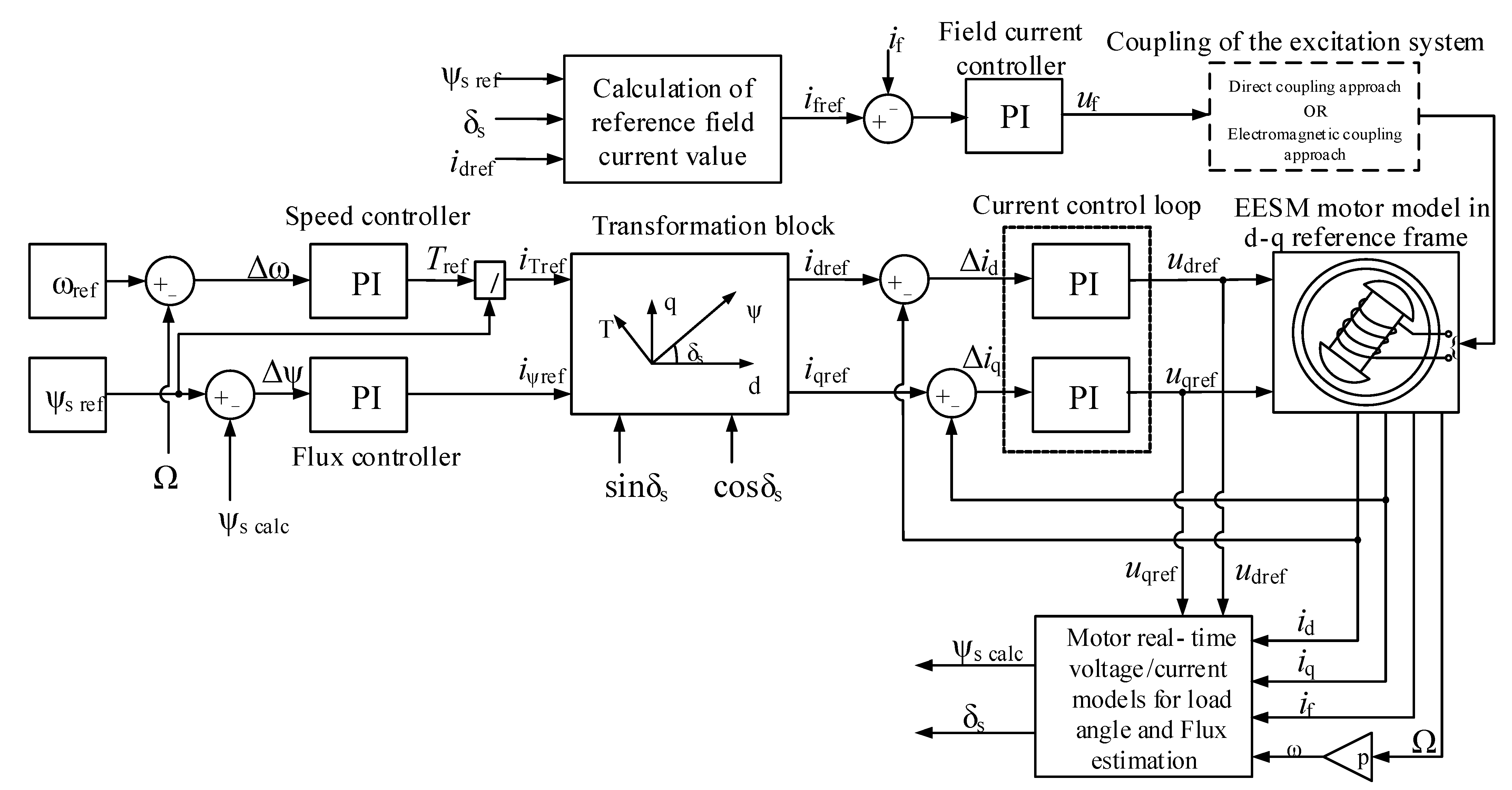
2.1. The EESM Model with Vector Control System

The EESM is modeled in d-q reference frame with vector control which include five PI controllers such as: speed controller, stator flux linkage controller, field current controller and two current controllers. Figure 1 shows a block diagram of an EESM model with a control system which consists of a real-time motor voltage/current model for calculation of load angle and stator flux linkage, transformation block for transforming stator quantities from T-ψ frame to d-q rotor frame and five proportional-integral (PI) controllers (according to which our study was based [18]). The data for EESM modeling is provided in Appendix A in absolute and relative units.

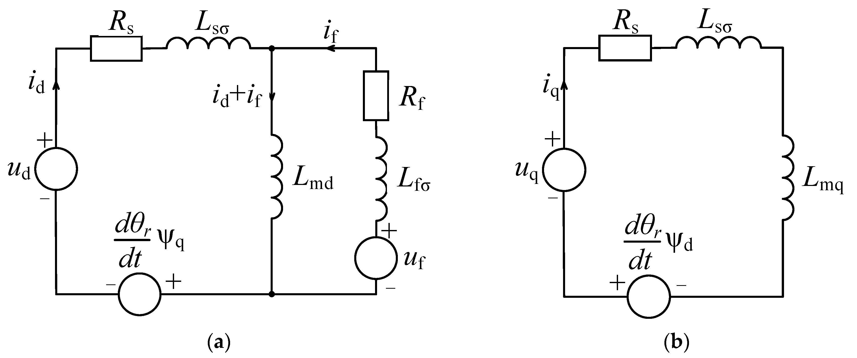
2.1.1. Modeling of the EESM

Three-phase EESM that is supposed to operate under the vector control is modeled using a two-axis theory in rotor reference frame, because it is more convenient to describe processes that take place in a synchronous machine with respect to the two most relevant magnetic orientations along the direct and quadrature axis.

For transformation of the EESM model from a three-phase coordinate system, the two-axis theory is applied to motor voltage model in three-phase coordinate system. For transformation of stator quantities from three-phase coordinate system into two-axis reference frame and vice versa, the Clarke–Park transformation is being used. The equations for transformation from three-phase system to the two-axes and to d-q reference frame is described in [18]. The model of EESM is described in d-q reference frame with the following system of voltage Equations (1)–(3) [18]:

$$u_d=R_s{i}_d+\frac{d{\psi }_d}{dt}-\frac{d{\theta }_r}{dt}{\psi }_q$$

(1)

$$u_q=R_s{i}_q+\frac{d{\psi }_q}{dt}+\frac{d{\theta }_r}{dt}{\psi }_d$$

(2)

$$u_f=R_f{i}_f+\frac{d{\psi }_f}{dt}$$

(3)

In the Equations (1)–(3), the $i_d$, $i_q$ and $u_d$, $u_q$ are the d-axis and q-axis components of the stator current and voltage; $u_f$—voltage of the field winding; $i_f$—the field winding DC current; ${\psi }_d$ and ${\psi }_q$ are the d-axis and q-axis components of the stator flux linkage; ${\psi }_f$—rotor flux linkage; ${\theta }_r$—rotor angle; $R_s$ and $R_f$ stator and field winding resistances, respectively.

Based on the system of Equations (1)–(3), the equivalent circuit of the EESM in rotor reference frame is presented in Figure 2. The advantage of the rotor reference frame is that the values of motor inductances remain constant during the change of the rotor position [18].

In Figure 2, $i_d$, $i_q$ and $u_d$, $u_q$ are the d-axis and q-axis components of the stator current and voltage; $u_f$ voltage of field winding; $i_f$ is the field winding DC current; $L_{md}$ and $L_{mq}$ direct and quadrature magnetizing inductances; $L_{\sigma s}$ leakage inductance of the stator; ${\psi }_d$ and ${\psi }_q$ are the d-axis and q-axis components of the stator flux linkage; $R_s$ and $R_f$ are stator and field winding resistances, respectively.

In order to model the EESM in the d-q reference frame, it is necessary to define the following motor parameters:

(1) $R_s$—stator resistance; (2) $L_{\sigma s}$—stator leakage inductance; (3) $L_{md}$—direct axis magnetizing inductance; (4) $L_{mq}$—quadrature axis magnetizing inductance; (5) $R_f^{\prime }$—rotor resistance referred to the stator side and (6) $L_f^{\prime }$—rotor leakage inductance referred to the stator side.

The inductances of synchronous motor model are calculated in the rotor reference frame as shown in Equations (4)–(6).

$$L_d=L_{md}+L_{\sigma s}$$

(4)

$$L_q=L_{mq}+L_{\sigma s}$$

(5)

$$L_f=L_{md}+L_{\sigma f}$$

(6)

where the magnetizing inductances ($L_{md}$, $L_{mq}$) were taken as constant values (the magnetic nonlinearity of EESM ferromagnetic materials was neglected due to EESM operation in a given operational point (i.e., magnetic linearization)). Based on Equations (4)–(6), the equations of flux linkages can be expressed in the rotor reference frame in Equations (7)–(9):

$${\psi }_d=L_{md}\left(i_d+i_f\right)+L_{\sigma s}{i}_d$$

(7)

$${\psi }_q=L_{mq}{i}_q+L_{\sigma s}{i}_q$$

(8)

$${\psi }_f=L_{md}\left(i_d+i_f\right)+L_{\sigma f}{i}_d$$

(9)

The electromagnetic torque $T_e$ for the given number of pole pairs $p$ is calculated according to Equation (10):

$$T_e=\frac{3}{2}p\left({\psi }_d{i}_q-{\psi }_q{i}_d\right)$$

(10)

2.1.2. Calculation of the Field Excitation Current

The control of field excitation current of the EESM is the essential task that should be adjusted according to the operational conditions of the electric motor. The field excitation current compensates the d-axis stator current and maintains the desired power factor of the stator [18]. Our mathematical model operates under the unity power factor control, in which reference value of the excitation current should be calculated according to Equation (11) [18]:

$$i_{f,ref}=\frac{\left|{\psi }_{s,ref}\right|\cos {\delta }_s-L_d{i}_{dref}}{L_{md}}$$

(11)

where ${\psi }_{s,ref}$ is the stator flux-linkage reference value and the ${\delta }_s$ is the load angle of the stator flux linkage. The current $i_{dref}$ is the reference d-axis current, obtained after the transformation block (Figure 1).

After the definition of the reference excitation current and the actual motor excitation current, the difference between the two is fed into the PI controller input (Figure 1) providing the excitation voltage reference for the motor model.

2.1.3. Transformation Block

The transformation block (Figure 1) is used for transformation from the air gap oriented current reference frame values (i.e., $i_{Tref}$ and $i_{\psi ref}$) to the rotor frame values (i.e., $i_{dref}$ and $i_{qref}$). The transformation is done using the following Expressions (12) and (13) [18]:

$$i_{dref}=i_{\psi ref}\cos {\delta }_s-i_{Tref}\sin {\delta }_s$$

(12)

$$i_{qref}=i_{\psi ref}\sin {\delta }_s+i_{Tref}\cos {\delta }_s$$

(13)

The current reference values (i.e., $i_{dref}$ and $i_{qref}$) obtained after the transformation are compared with the actual ones (i.e., $i_d$ and $i_q$) and the resulting error signal is fed into the current PI controllers (Figure 1).

2.1.4. Motor Voltage/Current Models

Motor real-time voltage and current models are important to implement in the EESM control system for the load angle ${\delta }_s$ calculation (21) and the estimation of the stator flux-linkage ${\psi }_{s,calc}$ (20) that is used as feedback value for the flux-linkage PI controller (Figure 1). Equations (18) and (19) are used for correction of the values obtained from voltage and current models and contain proportional and integral gains (i.e., $K_p$ and $K_i$). The necessity of using voltage (14) and (15) and current (16) and (17) models is conditioned by the fact that the voltage model is not applicable to zero speed and low-speed operation, where current model is used for correction of calculated load angle and stator flux linkage [18].

$${\psi }_{d\_u}={{\displaystyle \int }}^{ }\left(u_{dref}-R_s{i}_d+\omega {\psi }_q\right)\mathrm{dt}$$

(14)

$${\psi }_{q\_u}={{\displaystyle \int }}^{ }\left(u_{qref}-R_s{i}_q-\omega {\psi }_d\right)\mathrm{dt}$$

(15)

$${\psi }_{d\_i}=L_{md}\left(i_d+i_f\right)+L_{\sigma s}{i}_d$$

(16)

$${\psi }_{q\_i}=L_{mq}{i}_q+L_{\sigma s}{i}_q$$

(17)

$${\psi }_{d,calc}=K_p\left({\psi }_{d u}-{\psi }_{d i}\right)+K_i\left({\psi }_{d u}-{\psi }_{d i}\right)$$

(18)

$${\psi }_{q,calc}=K_p\left({\psi }_{q u}-{\psi }_{q i}\right)+K_i\left({\psi }_{q u}-{\psi }_{q i}\right)$$

(19)

$${\psi }_{s,calc}=\sqrt{{\psi }_{d,calc}^2+{\psi }_{q,calc}^2}$$

(20)

$${\delta }_s=arctan\frac{{\psi }_{q,calc}}{{\psi }_{d, calc}}$$

(21)

2.2. Selection of the EESM for Modeling and Analysis

Parameters of the Real EESM Used for Modeling

For the modeling of EESM, the parameters of the real three-phase synchronous generator have been used. Its rated values are: $S$ = 5.5 kVA, $U$ = 400 V (star connection), $f$ = 50 Hz, $n$ = 3000 rpm, $\cos \phi$ = 0.8. The modeled EESM-ET16F-130/A available in the Laboratory of Electrical Machines, UNI LJ, is shown in Figure 3. Detailed data of the EESM (given by the manufacturer and measured in the laboratory) are specified in the Appendix A,

Table A1. Modeling parameters of the three-phase synchronous generator ET16F-130/A from Mecc Alte S.p.A [26].

Parameters		Value (SI)	Value (pu)
Apparent power	S	5500 VA	1.0011
Nominal active power	Pn	4400 W	-
Nominal voltage	Un	400 V	1.2247
Nominal current	In	7.93 A	0.7071
Nominal field current	If_no_load Ifn	1.11 A 4.11 A	0.0711 0.2639
Nominal field voltage	Ufn	44 V	0.124
Stator winding resistance	Rs	1.5 Ω	0.0515
Field winding resistance without resistance of brushes	Rf	7.25 Ω	0.3378
Field winding time constant	τf	206.8 ms	-
Nominal frequency	f	50 Hz	-
Number of pole pairs	p	1	-
Moment of inertia	J	0.0129 kgm2	-
Power factor	cosφ	0.8	-
Nominal speed	n	3000 RPM	-

.

The measured inductance-excitation current profile of the EESM excitation windings for the complete range of the EESM excitation current is also provided in Appendix A, Figure A1.

2.3. The Wireless Power Transfer System Applied for the EESM Excitation

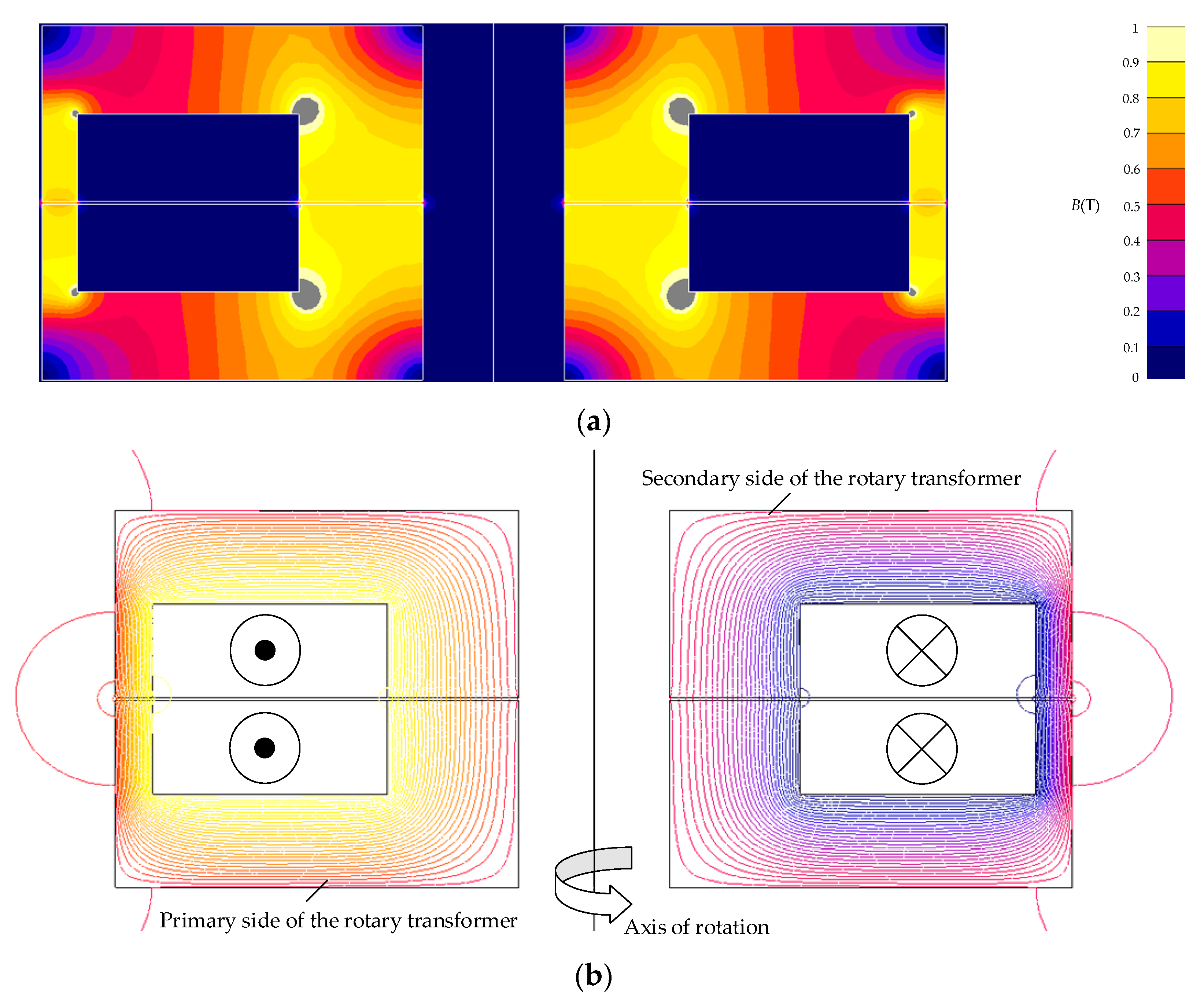
2.3.1. The Geometries of Wireless Power Transfer Systems Applied for EESM Excitation

The WPT technologies for the EESM excitation are, in general, performed via different couplings approaches such as: resonant inductive, inductive and capacitive. The solutions with the resonant coupling (i.e., via capacitor) contribute to the compensation of the reactive power and to the zero voltage switching in the inverter on the transformer’s primary side. However, the resonant topology on the rotating side may impose several drawbacks such as alterations of the secondary side voltage which within normal operation conditions (i.e., during the rotation) needs to be constant, with larger number of elements at the secondary side, etc. [17].

Based on the literature review [17], the inductive coupling via the rotary transformer is the most reliable and robust. Namely, for the EESM excitation, the single-phase rotary transformers are predominantly used due to their advantages such as high mechanical strength and small dimensions compared to other types. However, the three-phase rotary transformer is a preferable choice for industrial applications that require high power transfer and low speed (i.e., aerospace, wind power generator turbines, etc.).

The single-phase rotary transformer topologies being used in industry are predominantly based on the axial and radial topologies [17]. To enhance the transferred power, efficiency and to decrease the size, high supply frequency is used, as recently reported in [19,20,21]. However, the complexity of inverters and their high price are the major inconveniencies imposed by supply of high frequencies. It should be also noted that the operation of the rotary transformers within the higher frequency range requires the usage of the ferrite materials having poor mechanical strength under high speeds and temperatures [17].

Therefore, in this study, we specifically focused on analysis of the radial and axial rotary transformer topologies (Figure 4) for lower range of supply frequencies. The geometry of the single-phase axial and radial rotary transformers is shown in Figure 4a,b, respectively.

2.3.2. Analytical Approach for Modeling of Rotary Transformers

The voltage $V_{rms}$ across the transformer windings can be calculated assuming the sinusoidal waveforms of the voltages based on the Equation (22), derived from Faraday’s law [22]:

$$V_{rms}=\sqrt{2}\pi fN{B}_{max}{A}_{c1}$$

(22)

where $B_{max}$ is the maximum value of the magnetic flux density in T, f is the supply frequency in Hz; N is the number of turns of the windings and the $A_{c1}$ is the first effective cross-section area of the transformer core in m².

The $A_{c1}$ can be derived from Equation (22) and calculated according to Equation (23):

$$A_{c1}=\frac{P_{trans}}{\sqrt{2}\pi f{B}_{max}{A}_w{k}_{cu}J}$$

(23)

where $P_{trans}$ is the transferred power in W, $k_{cu}$ is the fill factor of the windings; J is the current density in the winding conductor which can be calculated as $J=I/S_w$, A/mm², where I is the conductor current in A and the $S_w$ is the conductor cross-section in mm² and the $A_w$ is the cross-section of the one side winding window area in mm² which can be calculated as $A_w=NI/k_{cu}J$.

The geometry of the modeled rotary transformers with the equivalent magnetic circuit model is depicted in Figure 5. The air gap $\delta$ and the magnetic paths’ lengths $l_c$ corresponding to the core segments (with their magnetic resistances $R_c$) are represented with the red line in Figure 5a,c (the indexes ‘cp’ and ‘cs’ represent the primary and the secondary side segments of the $l_c$ and $R_c$, respectively). The $A_{c1}$ marked in Figure 5a,c was calculated according to the Equation (23), while the $A_{c2}$ was calculated so as to be equal to $A_{c1}$ and $A_{c3}$ (Figure 5) in order to maintain equal magnetic flux across all three cross-sections (i.e., $A_{c1}$ =$A_{c2}$ = $A_{c3}$). This is an important sizing recommendation for the effective cross-section areas ($A_{c2}$) and ($A_{c3}$) of the rotary transformer ferromagnetic core, which was not reported in previous literature [12,22,23]. The winding area $A_w$ is marked in Figure 5a,c. The dimensions $r_{sh}$, $r_1$, $r_2$ and $r_3$ are: the shaft radius, the outer radius of the $A_{c1}$, the inner radius of the $A_{c2}$ and the outer radius of the $A_{c2}$, respectively. The magnetic reluctance circuit of the axial and radial rotary transformers are shown in Figure 5b,d. The magnetic reluctance circuit can be divided on the core segments and air gap segments, the number of which is usually dependent on the geometrical structure of the core. In Figure 5b,d, the reluctance circuit is divided in 14 core segments (7 segments correspond to one half of the core of the transformer), two air gap segments and two additional air gap segments that take into account leakage fluxes in winding area $A_w$.

One of the important objectives of the study is to model single-phase rotary transformer for different working frequencies in order to find the correlation between the supply frequency and the change in size/volume of the core of the rotary transformer. Namely, the dimensions of the modeled rotary transformers were determined for the following supply frequencies 50 Hz, 400 Hz and 1000 Hz. For the ferromagnetic core, the Cogent M250-35A material was used due to their desirable electromagnetic and mechanical properties at the frequencies lower than 2500 Hz and mature manufacturing technology which contribute to the robustness and cost-effectiveness of the rotary transformer. It should be noted that the modeling has been done for three different magnetic flux densities (i.e., B = 1 T, 1.3 T and 1.5 T) with the aim to investigate the influence of the magnetic flux density on the size/volume of the rotary transformer at different supply frequencies. The iron losses of the Cogent M250-35A for different frequencies were taken from the datasheet of the manufacturer [24] (the B(H) characteristic of the M250-35A is provided in Appendix B, Figure A2).

The cross-section area of the winding window $A_w$ and the size of the air gap were kept equal in both topologies (axial and radial) in order to more clearly compare the magnetic characteristics of both topologies. The parameters of the modeled rotary transformers are listed in

Table 1. Parameters of the modeled rotary transformers.

Parameters	Axial Rotary Transformer Topology	Radial Rotary Transformer Topology
Outer radius of the core (primary/secondary side)	$r_3$	$r_3$
Outer radius of the winding window	$r_2$	$r_2$
Inner radius of the winding window	$r_1$	$r_1$
Shaft radius	$r_{sh}$	$r_{sh}$
Height of the winding window	$l_N$	b
Width of the winding window	b	$l_N$
Width of the first main cross-section $A_{c1}$	$w_1$	$w_1$
Width of the second main cross-section $A_{c2}$	$w_2$	$w_2$
Width of the auxiliary cross-section $A_{c3}$	$w_3$	$w_3$
Air gap width	$\delta$	$\delta$
Winding window cross-section area	$A_w$	$A_w$
First main cross-section area of the ferromagnetic core	$A_{c1}$	$A_{c1}$
Second main cross-section area of the ferromagnetic core	$A_{c2}$	$A_{c2}$
Auxiliary cross-section area of the ferromagnetic core	$A_{c3}$	$A_{c3}$
Core material	Cogent M250-35A	Cogent M250-35A

and marked in Figure 5a,c.

The magnetic reluctances $R_c$ and $R_{gap}$ for the axial topology were calculated using Equations (24) and (25), respectively [23]:

$$\begin{array}{c}{R}_{cp1}=R_{cs1}=\frac{ln\left(r_{sh}+\left(b+w_2\right)-\left(w_2\right)/2\right)-ln\left(r_{sh}+w_2\right)}{2\pi {\mu }_0{\mu }_r{w}_3}\\ R_{cp2}=R_{cs2}=\frac{w_3}{2\pi {\mu }_0{\mu }_r\left({\left(r_{sh}+\left(r_3-r_{sh}\right)\right)}^2-{\left(r_{sh}+\left(r_3-r_{sh}\right)-w_2\right)}^2\right)}\\ R_{cp3}=R_{cs3}=\frac{w_3}{2\pi {\mu }_0{\mu }_r\left({\left(r_{sh}+w_1\right)}^2-r_{sh}{}^2\right)}\\ R_{cp4,6}=R_{cs4,6}=\frac{\left(b+w_3\right)}{2\pi {\mu }_0{\mu }_r\left({\left(r_{sh}+\left(r_3-r_{sh}\right)\right)}^2-{\left(r_{sh}+\left(r_3-r_{sh}\right)-w_2\right)}^2\right)}\\ R_{cp5,7}=R_{cs5,7}=\frac{\left(b+w_3\right)}{2\pi {\mu }_0{\mu }_r\left({\left(r_{sh}+w_1\right)}^2-r_{sh}{}^2\right)}\end{array}$$

(24)

$$\begin{array}{c}{R}_{gap1}=\frac{\delta }{\pi {\mu }_0\left({\left(r_{sh}+\left(r_3-r_{sh}\right)\right)}^2-{\left(r_{sh}+\left(r_3-r_{sh}\right)-w_2\right)}^2\right)}\\ R_{gap2}=\frac{\delta }{\pi {\mu }_0\left({\left(r_{sh}+w_1\right)}^2-{\left(r_{sh}\right)}^2\right)}\end{array}$$

(25)

The reluctances of the winding area $R_{\sigma p}$ and $R_{\sigma s}$ are equal and can be calculated according to the Equation (26):

$$R_{\sigma p}=R_{\sigma s}=\frac{3·\left(ln\left(r_{sh}+\left(r_3-r_{sh}\right)-w_2\right)-ln\left(r_{sh}+w_1\right)\right)}{2\pi {\mu }_0\left(b+2·\delta \right)}$$

(26)

The fringing flux factor $F_f$ in Equation (27) is implemented into Equation (25) to make the result more accurate in Equation (28) [23]:

$$F_f=1+\frac{A_f}{A_{c}k}$$

(27)

$$\begin{array}{c}{R}_{gap1}=\frac{\delta }{\pi {\mu }_0\left({\left(r_{sh}+\left(r_3-r_{sh}\right)\right)}^2-{\left(r_{sh}+\left(r_3-r_{sh}\right)-w_2\right)}^2\right)}·\frac{1}{F_f}\\ R_{gap2}=\frac{\delta }{\pi {\mu }_0\left({\left(r_{sh}+w_1\right)}^2-{\left(r_{sh}\right)}^2\right)}·\frac{1}{F_f}\end{array}$$

(28)

The cross-section area $A_f=A_{c}h-A_c$ takes into account only the fringing flux lines. The coefficient $h$ indicates the extension of the cross-section A_c area which occurs due to the fringing effect. The coefficient $k$ denotes the ratio between the extension of the magnetic path length due to the fringing flux and the actual air gap.

The self-inductance $L_{11}$ of the rotary transformer can be calculated according to Equation (29):

$$L_{11}=\frac{N_p^2}{R_{\sum }}$$

(29)

where $N_p$ and $R_{\sum }$ stand for the number of turns of the primary winding and the sum of all magnetic circuit reluctances of the rotary transformer (Figure 5).

The Equation (30) form [25] was used for the leakage inductance calculation of the transformer:

$$L_{\sigma 1}=L_{\sigma 2}=\frac{{\mu }_0{N}_p^2\pi R_{mean}}{l_N}\left(\delta +\frac{b_1+b_2}{3}\right)$$

(30)

where $R_{mean}$, $l_N$, $\delta ,$ $b_1$ and $b_2$ stand for the mean value of the radius between the primary and the secondary windings, the length of the transformer window and the air gap.

The equivalent electrical circuit of the single-phase rotary transformer and the relations between self-inductance, magnetizing inductance and leakage inductance are given in (Figure 6), where $R_p$ and $R_s$ are the primary and secondary side winding resistances; $L_m$ and $L_{11}$, $L_{22}$ magnetizing and self-inductances; ${\psi }_1$ and ${\psi }_2$ are the primary and the secondary flux linkages and $i_1$ and $i_2$ are the primary and secondary winding currents, respectively. The simplified electrical circuit of the single-phase rotary transformer is shown in Figure 6b (the transformer turns ratio in our case is one).

The efficiency of the power transfer of the rotary transformer is calculated according to Equation (31) [25]:

$$\eta =\frac{P_n}{P_n+P_{\mathrm{cu}}+P_{\mathrm{fe}}}$$

(31)

where $P_n$ is the calculated nominal power of secondary side of the rotary transformer, W; $P_{\mathrm{cu}}$—copper losses in primary and secondary windings, W; $P_{\mathrm{fe}}$—iron losses in transformer’s primary and secondary cores, W.

2.3.3. The Time Constant Determination of the Axial and Radial Rotary Transformers

The geometrical dimensions and number of turns of the rotary transformer were taken from the analytical calculations that were verified with the FEM models. The proper number of turns was derived from the cross-sectional area of the winding window, fill factor and current density for the primary and secondary side of the rotary transformer (Equation (23)). It should be noted that the number of turns was kept to the minimum in order to achieve the fast possible dynamic response of the inductive coupling. The time constant $\tau$ of the rotary transformer was calculated using Equation (32), by taking into account the modeled number of turns, geometrical and material properties [25].

$$\tau =\frac{L_m+L_{\sigma 1}+L_{\sigma 2}}{R_{\sum }}$$

(32)

where $L_m$—magnetizing inductance (Equation (29)) of the rotary transformer, H; $L_{\sigma 1}$, $L_{\sigma 2}$—leakage inductances of the rotary transformer, H and $R_{\sum }=R_p+R_s$—DC resistance of the primary and secondary windings of the rotary transformer, Ω. AC winding resistance, due to skin effect of the primary and secondary windings was neglected due to use of Litz wire.

The implementation of the rotary transformer model into the EESM model was realized as a transfer function (Equation (33)) that was derived from simplified equivalent circuit (Figure 6b) with the current time constant of the rotary transformer (Equation (32)) inserted into the excitation circuit with the aim to simulate the time delay imposed by electromagnetic coupling approach (as shown in Figure 1):

$$H\left(s\right)=\frac{1/R_{\sum }}{{\tau }_s+1}$$

(33)

In such a way, the influence of the rotary transformer’s design geometry and resistance of the windings were taken into account. Basically, by changing the magnetizing inductance that depends on the core design of the rotary transformer and resistance of the windings, the dynamic electric response of the control system can be modified.

2.4. Estimation of the Change in Dynamic Performance of the EESM Control System Due to the Wireless Power Transfer Excitation

The Method Used for Comparison of the Dynamic Performances between Direct and Electromagnetic Coupling Approaches

In order to perform the comparison between the dynamic response time of the direct coupling (i.e., modeled with simulation of brushes’ conductance in the excitation circuit) and the electromagnetic coupling approach (i.e., modeled with a time delay inserted into the excitation circuit as a transfer function) in vector control system of the EESM, the mathematical method using motor rotational speed signal was selected. The speed signal allows to trace the fast changes that occur in different operational conditions of the motor and to estimate the response time of the vector control system under the same load, but with different coupling approaches. The Root Mean Squared Error (RMSE) was used to compare the two signals obtained with direct and electromagnetic coupling approaches (34):

$$\mathrm{RMSE}=\sqrt{{\displaystyle \sum }_{i=1}^n\frac{{\left({\widehat{y}}_i-y_i\right)}^2}{n}}$$

(34)

where ${\widehat{y}}_i$—is the speed signal obtained with the direct contact approach; $y_i$—is the speed signal obtained with the electromagnetic coupling approach and $n$ is the number of samples.

We assumed that the rotational speed signal obtained from the model with direct coupling approach is a reference signal, while the rotational speed signal obtained from the model with electromagnetic coupling approach is experimental signal. According to the RMSE method, the experimental signal with the lowest numerical error represents the best fit to the reference signal (i.e., meaning that RMSE = 0% corresponds to ideal agreement between two signals, while RMSE = 100% means the worst case).

3. Results and Discussion

3.1. Results of the Axial and Radial Rotary Transformer Modeling

3.1.1. Design Methodology of the Axial and Radial Rotary Transformers with Different Supply Frequencies

The rotary transformer was modeled with the aim to obtain the following excitation requirements: $I_{exc\_\max \_DC}=5.7$ A at the field winding resistance $R_f=7.63$ Ω which corresponds to $U_{exc\_DC}=44$ V of the modeled EESM (Appendix A). The primary AC peak voltage value required for establishing these excitation conditions and for the compensation of the voltage drop due to the winding resistance and air gap leakage inductance will be $U_1=76$ V at all analyzed supply frequencies 50 Hz, 400 Hz and 1000 Hz. The primary AC voltage value depends on field winding parameters of the EESM and on the air gap width. The air gap width is kept equal in both topologies. The number of turns of the transformer’s primary winding the was calculated in such a way to establish the value of magnetic flux density around 1 T in the main cross-sections of the core (i.e., keeping constant magnetic flux density in the core is quite impossible due to leakage/fringing fluxes over winding window) at all supply frequencies. It should be noted that according to the Equation (23), the dimensions of the rotary transformer are significantly influenced by the change in cross-section of the winding area $A_w$ (i.e., by increasing the $A_w$, the dimensions of the rotary transformer will be reduced, as described by Equation (23)). As a result, the cross-section of one side winding area ($A_w=250$ mm²) is kept constant in both topologies (i.e., radial and axial) in order to perform a precise comparison between the two topologies. Moreover, the second main cross-section $A_{c2}$ and auxiliary cross-section area $A_{c3}$ are kept equal to the first main cross-section $A_{c1}$ of the ferromagnetic core (i.e., $A_{c1}=A_{c2}=A_{c3}$) in all cases of the supply frequency.

The dimensions and electric parameters obtained from the analytical calculations of axial and radial rotary transformers for three different supply frequencies are summarized in

Table 2. Dimensions and electrical parameters of the axial and radial rotary transformers.

Parameters	Axial Rotary Transformer Topology			Radial Rotary Transformer Topology
Supply frequency	50 Hz	400 Hz	1000 Hz	50 Hz	400 Hz	1000 Hz
$r_3$	103 mm	51 mm	42 mm	99 mm	47 mm	38 mm
$r_2$	84 mm	47 mm	40 mm	69 mm	32 mm	25 mm
$r_1$	59 mm	22 mm	15 mm	59 mm	22 mm	15 mm
$r_{sh}$	8 mm	8 mm	8 mm	8 mm	8 mm	8 mm
$l_N$	25 mm	25 mm	25 mm	25 mm	25 mm	25 mm
$b$	10 mm	10 mm	10 mm	10 mm	10 mm	10 mm
$w_1$	51 mm	14 mm	7 mm	51 mm	14 mm	7 mm
$w_2$	19 mm	4 mm	2 mm	19.7 mm	4.7 mm	2.7 mm
$w_3$	29 mm	10 mm	6 mm	29 mm	10 mm	6 mm
δ	0.3 mm	0.3 mm	0.3 mm	0.3 mm	0.3 mm	0.3 mm
Total volume	2.4 × 10−3 m3	2.1 × 10−4 m3	0.845 × 10−4 m3	2.4 × 10−3 m3	2.59 × 10−4 m3	1.28 × 10−4 m3
Turns (primary/secondary)	33/33	33/33	33/33	33/33	33/33	33/33
Winding DC resistance (primary/secondary)	0.1361 Ω/0.1361 Ω	0.0657 Ω/0.0657 Ω	0.0524 Ω/0.0524 Ω	0.1414 Ω/0.1218 Ω	0.071 Ω/0.0514 Ω	0.0577 Ω/0.0381 Ω

.

From the data listed in Table 2, it can be seen that the increase of the supply frequency reduces the volume of the rotary transformer. It should be noted that both topologies (axial and radial) are characterized with the same dimensions of the first main cross-section area $A_{c1}$. However, the axial rotary transformer has a larger area of flux path in comparison to the radial topology. The increase of frequency from 50 Hz to 400 Hz (i.e., 8 times increased frequency) reduces the volume of the axial topology by 11.4 times, while the volume of the radial topology is reduced by 9.2 times. For the increase of frequency from 400 Hz to 1000 Hz (i.e., 2.5 times increased frequency), the reduction of the volume are the following: axial—2.48 times and radial—2.02 times. The obtained results show that the reduction of the transformer volume is proportional to the increase of the supply frequency in both topologies. Moreover, the raise of supply frequency with the aim to reduce the volume of the rotary transformer’s core will reach a plateau value at further increase towards higher frequencies. This dependency is shown in Figure 7 for different values of magnetic flux density in the core. The profile of the volume vs. frequency curve shown in Figure 7 is the result of the imposed limitation of the transformer’s core dimensions to integer values. As expected, the reduction of volume as a function of frequency decays exponentially and after reaching 1000 Hz, the reduction of volume of the rotary transformer became almost negligible (Figure 7b). The results indicate that for the frequencies above 1000 Hz, the rotary transformer’s volume reaches a plateau and the increase of the supply frequency would result in the following drawback such as: higher price and complexity of high frequency inverter, increase of iron losses, not efficient usage of the material, etc.

Another approach to obtain smaller dimensions at frequencies up to 1000 Hz is to maintain higher value of magnetic flux density in the transformer’s core (Figure 7a). The increase of the magnetic flux density allows for further reduction of the rotary transformer volume (frequency range up to 500 Hz), as can be seen from Figure 7a. However, special attention should be paid to the choice of the core material, so as not to reach the high saturation of the material during the transformer’s operation.

3.1.2. The Comparison of the Analytical Models with Numerical Modeling of the Axial and Radial Rotary Transformers Topologies

The verification of analytical results with numerical simulations was done for the radial and axial rotary transformer’s topologies with the dimensions specified in Table 2. The following output parameters of the rotary transformers have been compared: magnetizing inductance $L_m$, leakage inductance $L_{\sigma }$ and rotary transformer’s time constant $\tau$.

The leakage inductance $L_{\sigma }$ obtained from the finite element analyses was calculated based on the electrical circuit of the single-phase rotary transformer (Figure 6a) described by the following Equations (35)–(37):

$$L_{\sigma 1}=L_{11}-L_m$$

(35)

$$L_{11}=\frac{{\psi }_1}{I_1}$$

(36)

$$L_m=\frac{{\psi }_2}{I_1}$$

(37)

where ${\psi }_1$ and ${\psi }_2$ are the primary and the secondary flux linkages, respectively and $I_1$ is the primary current.

The specific iron losses of the core material (i.e., Cogent M250-35A) used in the numerical models were taken from the manufacturer’s datasheet [24]. The comparison between the analytical and numerical results is given in

Table 3. Dimensions and electric parameters of the axial and radial rotary transformers.

Parameters	Analytical Calculation	Numerical Calculation	Analytical Calculation	Numerical Calculation	Analytical Calculation	Numerical Calculation
	Axial rotary transformer topology
	50 Hz		400 Hz		1000 Hz
$L_m$	24.3 mH	25.5 mH	3.1 mH	3.31 mH	1.3 mH	1.46 mH
$L_{\sigma 1}$	85.66 μH	85.28 μH	41.33 μH	40.56 μH	32.94 μH	31.94 μH
$L_{\sigma 2}$	85.66 μH	85.28 μH	41.33 μH	40.56 μH	32.94 μH	31.94 μH
$L_{\sigma }=L_{\sigma 1}+L_{\sigma 2}$	171.32 μH	170.56 μH	82.66 μH	81.12 μH	65.88 μH	63.88 μH
τ	89.9 ms	94.3 ms	23.9 ms	25.8 ms	13.3 ms	14.54 ms
	Radial rotary transformer topology
$L_m$	29.3 mH	29.15 mH	5.1 mH	4.8 mH	2.6 mH	1.89 mH
$L_{\sigma 1}$	89.01 μH	86.08 μH	44.69 μH	41.71 μH	36.3 μH	40.57 μH
$L_{\sigma 2}$	76.67 μH	79.4 μH	32.35 μH	34.87 μH	23.96 μH	15.19 μH
$L_{\sigma }=L_{\sigma 1}+L_{\sigma 2}$	165.68 μH	165.48 μH	77.04 μH	76.58 μH	60.26 μH	55.76 μH
τ	111.9 ms	111.4 ms	42.4 ms	39.84 ms	27.8 ms	20.31 ms

. In all analytical calculations shown in Table 3, the maximum value of the magnetic flux density in the core was maintained at 1 T. This means that the inductance $L_m$ can be considered almost constant, which reflects the non-saturated condition in the core (i.e., linear part of the B(H) curve, which we maintained at 1 T).

From the comparison of the magnetizing inductance and leakage inductance of the WPT, it can be seen that for the axial topology of the rotary transformer, the calculation difference does not exceed 12%, which verified the analytical model. The difference in radial rotary transformer topology remains in the range of 10%. However, at the supply frequency 1000 Hz, the difference between the analytically and numerically calculated magnetizing inductance and secondary side leakage inductance reaches 50%. This difference between the analytical and numerical results occurs due to a smaller cross-section of the magnetic flux path in comparison to the axial topology designed for the same supply frequency, which leads to local saturations along the radial magnetic path in the numerical models of the transformer core. These local saturations are not taken into account in the analytical models.

In Figure 8, the relationship between the current time constants and the supply frequency is shown for both rotary transformer topologies. As it was mentioned before, the step change profile of the time constant is a result of the limitation of the main dimensions to the integer values and in the case of axial rotary transformer topology, the inductance changes proportionally with the reduction of the winding resistance. Meanwhile, in the case of radial rotary transformer topology, the inductance and resistance change is not proportional to each other, due to the geometrical asymmetry of the primary and secondary sides of the rotary transformer. Table 3 shows that the highest time constants are obtained for the radial topology of the rotary transformer (Figure 8b) compared to the time constant of the axial topology. Highest time constants are obtained due to larger values of the magnetizing inductances of the radial topology transformers compared to the axial rotary transformer for the same supply frequency (Table 3).

The results shown in Figure 8 indicate that the value of the time constant is exponentially decaying with the supply frequency up to 1500 Hz and remains almost constant above this value. The same functional dependency was also found for the volume with respect to the supply frequency (Figure 7).

The analytically determined time constants of the axial and radial rotary transformers listed in Table 3 will be later used for the simulations of the wireless power transfer (WPT) system in the EESM model with the vector control system.

The magnetic flux density and flux lines’ distribution in the core of axial rotary transformer topology is shown in Figure 9. The results are shown only for the transformer designed for the supply frequency 400 Hz, since it has the best performance in terms of volume/optimum size and smallest iron losses (Table 3).

From Figure 9a, it can be seen that the magnetic flux density in the core is maintained around 1 T. The magnetic flux density exceeds the desired value within the area at the edges of the winding window (Figure 9a). In Figure 9b, the flux lines in the core of the rotary transformer are shown. The lines confined inside the core represent the main magnetic flux, leakage flux is shown with lines that close inside the winding window (in Table 3, the leakage fluxes are represented in the form of leakage inductances), while the lines that extend beyond the core structure in the vicinity of air gap represent the fringing effect of the air gap. The leakage flux can be reduced by optimizing the geometry to such an extent that the leakage inductance and the fringing effect will be as low as possible (e.g., by considering different shapes and positioning of the pot cores of the rotary transformer).

It should be also noted that analytical and finite element method modeling does not allow to take into account the effects of the manufacturing processes of the laminated core of the rotary transformer (i.e., in the case of laminated core, we could not achieve equal magnetic conductivities in radial and axial directions inside the transformer’s core). Hence, it is impossible to precisely estimate the iron losses and consequently, the efficiency of the rotary transformer with laminated core. The possible solution could be the usage of a material that has homogenous structure such as, for example, ferrites or soft magnetic composites. However, by taking into account that the ferrites are meant to be used in the magnetic structures at high frequencies and low value of magnetic flux density, the soft magnetic composites could be a more preferable choice for the core of the rotary transformer (rotational mechanical properties should be also taken into account when analyzing the use of soft magnetic material). In addition, for special shapes of the rotary transformers requiring high working frequencies, amorphous materials could also be used in order to minimize the iron losses.

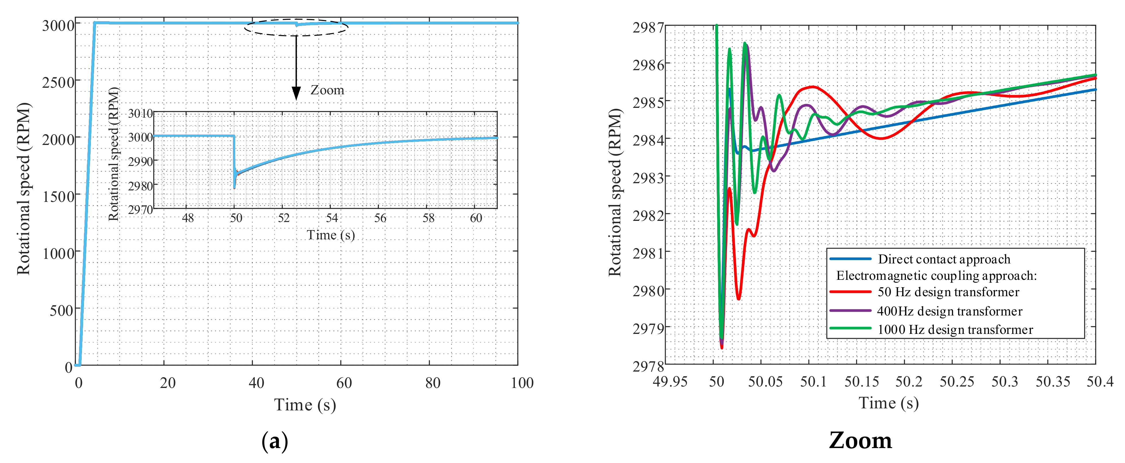
3.2. Modeling Results of the EESM Control System with Rotary Transformer (i.e., WPT) and Comparison to the Conventional Excitation (i.e., Sliding Contacts)

Modeling of the EESM with control system in d-q reference frame was conducted in MATLAB/Simulink software according to the Equations (1)–(21). The PI controllers were tuned manually in two stages: firstly, the inner current loop with excitation circuit was tuned and secondly, outer loop with speed and flux regulators was tuned. After obtaining the reference results that describe the operation conditions of the EESM with direct contact approach (i.e., model with simulation of brushes’ conductance in the excitation winding circuit), the transfer function of the rotary transformer (i.e., by which the time delay (Equation (33)) is imposed) was inserted into the excitation winding circuit to simulate the electromagnetic coupling approach of the rotary transformer. It should be noted that values of the PI gains of field current controller were kept the same as in the case for direct contact approach with the aim to observe the influence of the rotary transformer design parameters (i.e., the rotary transformer time constant) on the dynamic performance of the EESM.

Figure 10 demonstrates the speed and torque curves of the EESM with direct contact approach and electromagnetic coupling approach using the time constants of the axial rotary transformer topology designed for supply frequencies 50 Hz, 400 Hz and 1000 Hz (with parameters represented in Table 3). The no-load start-up with further addition of the load 5 Nm at 50 s was simulated. From Figure 10, it can be seen that the dynamic performance (i.e., response time) was slightly increased in comparison with the model based on direct contact approach; also, due to electromagnetic coupling, the transient processes are increased. The control response of the EESM model with rotary transformer designed with supply frequencies 50 Hz, 400 Hz and 1000 Hz (Table 3) are characterized with bigger speed drop due to a more oscillated transient process which can be seen from the change in speed curve (Figure 10a) and smaller overshoot in torque curve (Figure 10b). Such behavior was predictable due to the slowest response of the PI field current controller (i.e., not adjusted PI controller gains), while operating via electromagnetic coupling approach.

To quantify the difference in response time between direct contact approach and electromagnetic coupling approach, the Root Mean Squared Error (RMSE) method is used. We assumed that the speed signal from the model with direct coupling approach is a reference signal and the speed signal from the model with electromagnetic coupling approach is the experimental signal. According to the RMSE principle, the experimental signal with the lowest error fits best to the reference signal. The speed signal (Figure 10a) shows that the Root Mean Squared Error (RMSE) between the model with direct contact approach and the rotary transformer with time constant 23.9 ms is equal to 5.38%, which in comparison with other rotary transformers’ results (

Table 4. The time constants of the rotary transformers at different supply frequencies and their RMSE error.

Supply Frequency of the Rotary Transformer	Rotary Transformer’s Parameters
Axial rotary transformer	Time constant value (τ)	RMSE (Δ)
50 Hz	89.9 ms	7.86%
400 Hz	23.9 ms	5.38%
1000 Hz	13.3 ms	6.06%
Radial rotary transformer	Time constant value (τ)	RMSE (Δ)
50 Hz	111.9 ms	8.76%
400 Hz	42.4 ms	6.16%
1000 Hz	27.8 ms	6.43%

) has the smallest RMSE error.

The changes of the excitation voltage can be seen from Figure 11 for both types of excitation. From excitation voltage curves, the information about the voltage limitations and voltage reserve of the rotary transformer in different operating conditions can be obtained. The spikes in first calculation steps in torque and excitation voltage curves in Figure 10b and Figure 11 are related to the inaccuracies of the motor voltage and current models that estimate the values of stator flux linkage and the load angle of the EESM.

In addition to the mathematical modeling, the experimental measurements have been performed as a preliminary experimental investigation to compare the direct (via brushes) and wireless (via transformer) excitation approaches of the EESM (EESM-ET16F-130/A motor). The influence of the rotary transformer on the EESM excitation winding was experimentally analyzed with the measurements using a conventional transformer with similar inductances and winding resistances to the modeled rotary transformer (Appendix C, Figure A4). The experimental measurements have been performed in order to emulate and predict the behavior of the modeled rotary transformer. The results of the experimental measurements indicated that the time constants of the EESM excitation current were almost the same for both approaches: with direct contact approach and with the wireless excitation using the conventional transformer (Appendix C, Figure A4). It should be noted that the time constant of the excitation current obtained with the presence of the transformer in the EESM excitation circuit comprises also the resistance of the brushes. If the resistance of the brushes would be eliminated from the time constant of the wireless excitation (as we did in the theoretical/mathematical model), the response time would be even shorter compared to the response time of the direct contact approach which confirms our calculations obtained with the mathematical modeling (i.e., Figure 10). More precise experimental measurements are planned to be performed within the frame of our future research work on a real rotary transformer prototype which we plan to build using the results presented in this study.

The simulations of the EESM model in Simulink were performed for all supply frequencies: 50 Hz, 400 Hz and 1000 Hz of axial and radial rotary transformers’ topologies in order to define the rotary transformer design that will decrease the influence of the electromagnetic coupling to the tolerable/acceptable level (i.e., transient behavior of the rotary transformer corresponding the most to the transient of the model with brushes). This is determined by the lowest RMSE value between EESM model with brushes and electromagnetic coupling. The results are given in Table 4.

From Table 4, it can be seen that the smallest difference between the electromagnetic coupling approach (i.e., rotary transformer) and the direct contact approach (i.e., brushes; speed reference signal) was obtained with the rotary transformer design with the time constant 23.9 ms at the supply frequency 400 Hz. In this case, the lowest RMSE value was obtained (5.38%) indicating the best dynamic performance in comparison to dynamic behavior obtained with other topologies of the rotary transformers at different frequencies (Table 4). It should be also noted that the further improvement of the dynamic performance of the EESM can be obtained by advanced adjustment of the PI gains of the field current controller.

4. Conclusions

In the present study, the mathematical model of the EESM with vector control system was built and upgraded with the equivalent model of the rotary transformer for wireless excitation of the rotor winding. Two different topologies of the rotary transformers (axial and radial) were analytically and numerically modeled and their influence on the response time of the EESM vector control system were assessed. The comparison of the dynamic performance of the EESM with wireless power transfer system (i.e., rotary transformer) to the direct contact approach (i.e., slip rings/brushes) was performed.

Based on the obtained results, the following conclusions can be derived:

-

The axial topology of the rotary transformer outperforms the radial type, since the minimum size with the best magnetic properties can be obtained with the axial topology of the rotary transformer for the same supply frequency. Namely, our results show that the best design in terms of size, time constant and inductance values can be obtained with the axial rotary transformer topology at the supply frequency of 400 Hz. In addition, the rotary transformer supplied with 400 Hz enables the usage of the classic H-bridge inverter which is an important advantage in terms of cost-effectiveness of the WPT system, while at higher frequencies (e.g., 1000 Hz), a special and more expensive high frequency inverter is required.

-

The comparison of the analytical and numerical results in 12% difference for both topologies (axial and radial). Thus, the developed analytical tool can be used as an efficient alternative for time-consuming numerical simulations.

-

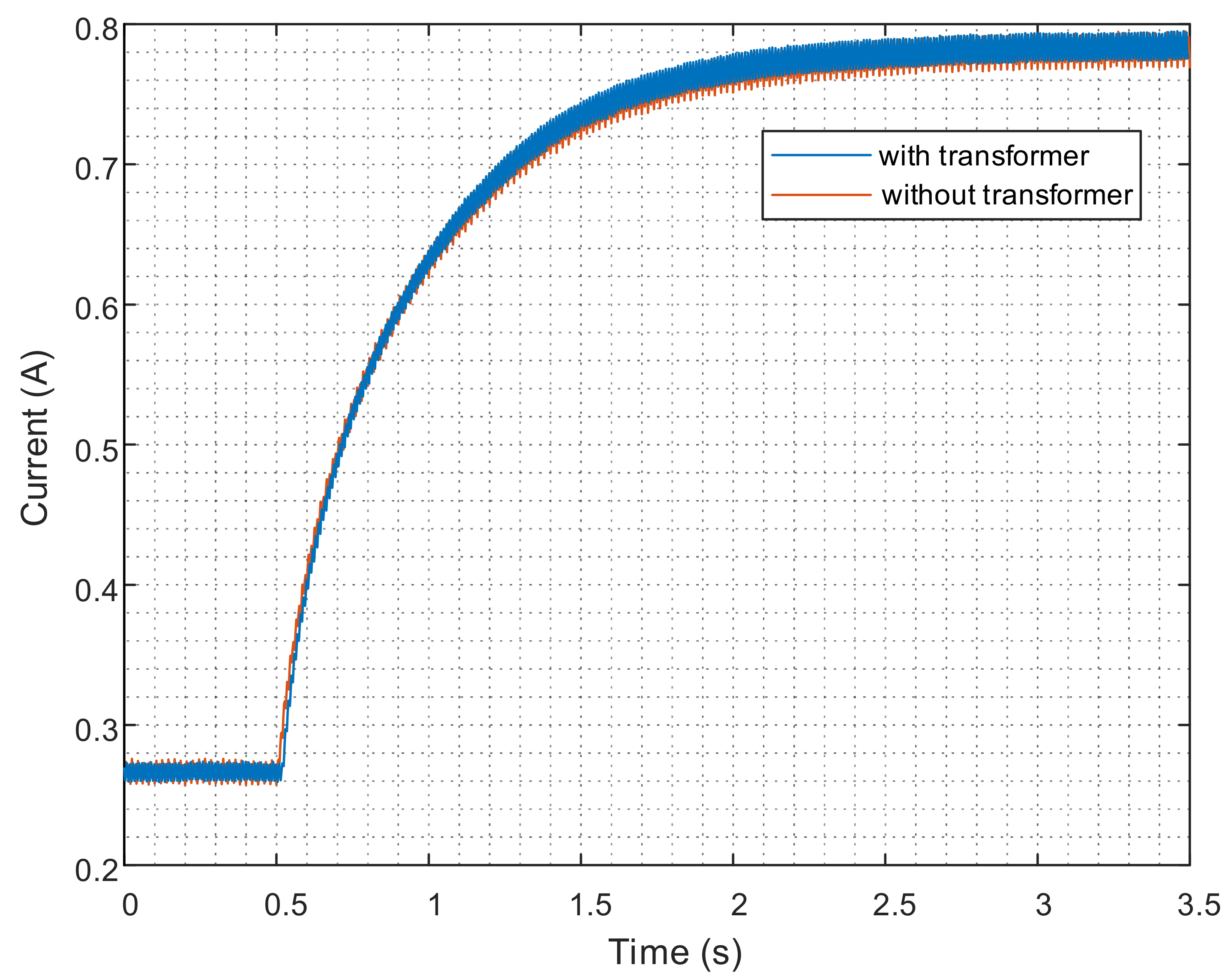
The usage of the rotary transformer instead of direct contact degrades the dynamic performance of the EESM by less than 5.38% in the case of 400 Hz design of the rotary transformer. Further improvement of the dynamic response of the EESM with rotary transformer can be achieved with the proper adjustment of the PI controllers’ gains of the control system. The future work towards improvement of the EESM dynamic response can also include the advanced optimization procedure for tuning the PI gains of the model controllers including the automatic recalculation of the geometry of the rotary transformer based on the rotary transformers’ time constant as an optimization goal. These results may have an important contribution in the field of the development of the power electronics required for the excitation circuits of the EESM.

Finally, the results we report here provide useful recommendations on proper design of the rotary transformer properties needed for the EESM excitation system, such as type of the rotary transformer—radial or axial, supply frequency, the geometrical and material properties of the ferromagnetic core and winding resistances.

References

1. EU European Commission. EU Climate Action and the European Green Deal. Available online: https://ec.europa.eu/clima/policies/eu-climate-action_en (accessed on 11 October 2021).
2. EEA Database on Climate Change Mitigation Policies and Measures in Europe. Available online: http://pam.apps.eea.europa.eu (accessed on 11 October 2021).
3. Amann, M.; Borken-Kleefeld, J.; Cofala, J.; Hettelingh, J.-P.; Heyes, C.; Hoglund, L.; Holland, M.; Kiesewetter, G.; Klimont, Z.; Rafaj, P.; et al. The final policy scenarios of the EU Clean Air Policy Package; TSAP Report #11; International Institute for Applied Systems Analysis (IIASA): Laxenburg, Austria, 2014. [Google Scholar]
4. Standard IEC 60349-2; Electric Traction—Rotating Electrical Machines for Rail and Road Vehicles—Part 2: Electronic Converter-fed Alternating Current Motors. IEC: London, UK, 2010.
5. Wang, Z.; Ching, T.W.; Huang, S.; Wang, H.; Xu, T. Challenges Faced by Electric Vehicle Motors and Their Solutions. IEEE Access 2021, 9, 5228–5249. [Google Scholar] [CrossRef]
6. Karki, A.; Phuyal, S.; Tuladhar, D.; Basnet, S.; Shrestha, B.P. Status of pure electric vehicle power train technology and future prospects. Appl. Syst. Innov. 2020, 3, 35. [Google Scholar] [CrossRef]
7. Staton, D.A.; Goss, J. Open source electric motor models for commercial EV & Hybrid traction motors. Presented at Coil Winding, Insulation & Electrical Manufacturing Exhibition (CWIEME), Berlin, Germany, 20–22 June 2017. [Google Scholar]
8. Popescu, M.; Goss, J.; Staton, D.A.; Hawkins, D.; Chong, Y.C.; Boglietti, A. Electrical Vehicles—Practical Solutions for Power Traction Motor Systems. IEEE Trans. Ind. Appl. 2018, 54, 2751–2762. [Google Scholar] [CrossRef] [Green Version]
9. Krings, A.; Monissen, C. Review and Trends in Electric Traction Motors for Battery Electric and Hybrid Vehicles. In Proceedings of the 2020 International Conference on Electrical Machines (ICEM), Gothenburg, Sweden, 23–26 August 2020; pp. 1807–1813. [Google Scholar]
10. Čorović, S.; Miljavec, D. Modal Analysis and Rotor-Dynamics of an Interior Permanent Magnet Synchronous Motor: An Experimental and Theoretical Study. J. Appl. Sci. 2020, 10, 5881. [Google Scholar] [CrossRef]
11. Maga, D.; Zagirnyak, M.; Miljavec, D. Additional losses in permanent magnet brushless machines. In Proceedings of the EPE-PEMC 2010—14th International Power Electronics and Motion Control Conference, Ohrid, Macedonia, 6–8 September 2010; pp. S412–S413. [Google Scholar] [CrossRef]
12. Illiano, E.M. Design of a Highly Efficient Brushless Current Excited Synchronous Motor for Automotive Purposes. Ph.D. Thesis, ETH Zurich, Zürich, Switzerland, 2014. [Google Scholar]
13. Di Gioia, A.; Brown, I.P.; Nie, Y.; Knippel, R.; Ludois, D.C.; Dai, J.; Hagen, S.; Alteheld, C. Design and Demonstration of a Wound Field Synchronous Machine for Electric Vehicle Traction with Brushless Capacitive Field Excitation. IEEE Trans. Ind. Appl. 2018, 54, 1390–1403. [Google Scholar] [CrossRef]
14. Tang, J.; Liu, Y.; Sharma, N. Modeling and Experimental Verification of High-Frequency Inductive Brushless Exciter for Electrically Excited Synchronous Machines. IEEE Trans. Ind. Appl. 2019, 55, 4613–4623. [Google Scholar] [CrossRef]
15. Paszek, S.; Boboń, A.; Berhausen, S.; Majka, Ł.; Nocoń, A.; Pruski, P. Synchronous Generators and Excitation Systems Operating in a Power System; Springer International Publishing: Cham, Switzerland, 2020. [Google Scholar]
16. Ruuskanen, V.; Niemelä, M.; Pyrhönen, J.; Kanerva, S.; Kaukonen, J. Modelling the brushless excitation system for a synchronous machine. IET Electr. Power Appl. 2009, 3, 231–239. [Google Scholar] [CrossRef]
17. Manko, R.; Čorović, S.; Miljavec, D. Analysis and Design of Rotary Transformer for Wireless Power Transmission. In Proceedings of the 2020 IEEE Problems of Automated Electrodrive. Theory and Practice (PAEP), Kremenchuk, Ukraine, 21–25 September 2020; pp. 1–6. [Google Scholar]
18. Pyrhonen, J.; Hrabovcova, V.; Scott Semken, R. Electrical Machine Drives Control: An Introduction; John Wiley & Sons: Chichester, UK, 2016; p. 504. [Google Scholar]
19. Zhang, Y.; Yang, J.; Jiang, D.; Li, D.; Qu, R. Design, manufacture, and Test of a Rotary Transformer for Contactless Power Transfer System. IEEE Trans. Magn. 2022, 58, 8400206. [Google Scholar] [CrossRef]
20. Toscani, N.; Brunetti, M.; Carmeli, M.S.; Castelli Dezza, F.; Mauri, M. Design of a Rotary Transformer for Installations on Large Shafts. J. Appl. Sci. 2022, 12, 2932. [Google Scholar] [CrossRef]
21. Bastiaens, K.; Krop, D.C.; Jumayev, S.; Lomonova, E. A Optimal design and comparison of high-frequency resonant and non-resonant rotary transformers. Energies 2020, 13, 929. [Google Scholar] [CrossRef] [Green Version]
22. Littau, A.; Wagner, B.; Köhler, S.; Dietz, A.; Weber, S. Design of Inductive Power Transmission into the Rotor of an Externally Excited Synchronous Machine. In Proceedings of the Conference on Future Automotive Technology (CoFAT), Munich, Germany, 17–18 March 2014. [Google Scholar]
23. Perrottet, M. Transmission Électromagnétique Rotative D’énergie et D’information Sans Contact. Ph.D. Thesis, EPLF, Lausanne, Switzerland, January 2000. [Google Scholar]
24. Datasheet of Cogent M250-35A Material. Available online: https://www.tatasteeleurope.com/sites/default/files/m250-35a.pdf (accessed on 10 December 2021).
25. Voldek, A.I. Electricheskie Mashiny, 2nd ed.; Energiya: Sankt-Peterburg, Russia, 1974; p. 350. [Google Scholar]
26. Datasheet on Three-Phase Synchronous Generator Mecc Alte ET16F-130/A. Available online: https://www.meccalte.com/downloads/ET16F.pdf (accessed on 10 December 2021).
Figure 1. Block diagram of vector control system of the EESM. (Parameters appearing in Figure 1 are explained in the following subchapters) [18].
Energies 15 02832 g001
Figure 2. The equivalent circuit of the EESM (a) in the d-axis direction referred to the stator winding; (b) in the q-axis direction referred to the stator winding.
Energies 15 02832 g002
Figure 3. The modeled EESM-ET16F-130/A (i.e., a real electrical machine available in the Laboratory of Electrical Machines, UNI LJ).
Energies 15 02832 g003
Figure 4. The modeled single-phase rotary transformer topologies: (a) axial and (b) radial. (The air gap width in the figures between the secondary and primary parts of the rotary transformers is intentionally enlarged for demonstrational purposes).
Energies 15 02832 g004
Figure 5. The modeled rotary transformers: (a) single-phase axial rotary transformer; (b) magnetic reluctance equivalent circuit of the single-phase axial rotary transformer topology; (c) single-phase radial rotary transformer and (d) magnetic reluctance equivalent circuit of the single-phase radial rotary transformer topology.
Energies 15 02832 g005aEnergies 15 02832 g005b
Figure 6. Equivalent electric circuit (a) and simplified equivalent electric circuit (b) of the single-phase rotary transformer [22].
Energies 15 02832 g006
Figure 7. Frequency dependence of the rotary transformer volume for axial topology calculated for three different magnetic flux densities (B = 1 T, 1.3 T and 1.5 T): (a) whole frequency range with zoomed area at the frequency interval 0–500 Hz; (b) zoomed area at the frequency interval 500–2500 Hz.
Energies 15 02832 g007
Figure 8. The calculated profile of the time constant vs. supply frequency for the axial (a) and radial (b) topology.
Energies 15 02832 g008
Figure 9. Magnetic flux density distribution (a) and flux lines’ distribution (b) in the core of axial rotary transformer with the supply frequency 400 Hz. With “cross” and “dots”, the direction of the current in the windings of the rotary transformer have been marked.
Energies 15 02832 g009
Figure 10. Comparison of speed (a) and torque (b) curves of the EESM operation with direct contact approach and electromagnetic coupling approach.
Energies 15 02832 g010aEnergies 15 02832 g010b
Figure 11. Comparison of excitation voltage curves of the EESM during transients with direct contact approach and electromagnetic coupling approach.
Energies 15 02832 g011