Abstract
The self-oscillation of the cavitating vortices is one of the dangerous phenomena of hydraulic turbine operation near full-load conditions. This work is an attempt to generalize data and expand insight on the phenomenon of self-excited oscillations by comparing the experimental results obtained on a simplified turbine and scaled-down pump–turbine models. In both cases, a series of high-speed imaging was carried out, which made it possible to study these phenomena with high temporal resolution. The high-speed imaging data was subjected to additional processing such as binarization, cropping, and scaling. For a simplified turbine model, the volume of the vapor cavity was calculated based on the assumption of the axial symmetry of the cavity, after which fast Fourier transform (FFT) analysis was carried out. A proper orthogonal decomposition (POD) analysis was also performed to examine individual modes in the original digital imaging data. For the pump–turbine, visualization data on the cavitation cavity oscillations were supplemented by pressure measurements in the draft tube cone to determine the frequency characteristics. Based on obtained experimental data, an improved one-dimensional model describing the oscillations of the cavitation cavity arising behind the hydraulic turbine runner is proposed.
1. Introduction
Swirling flows are widespread in industrial applications. They provide the separation of solid particles from the gaseous phase into cyclone separators, stabilize the flames, and create a wide recirculation zone for better fuel mixing in vortex burners. In a hydraulic turbine, the swirling flow can be observed under off-design part-load flow rate conditions, which are usually required for grid regulation. The diversity of the phenomena related to swirl intensity, including the formation of the recirculation zone and the non-stationary or quasi-stationary vortex structures, have attracted the attention of researchers over the years. Moreover, when dealing with a multiphase swirling flow, such as cavitation flows, the study becomes much more complicated. For example, the two-phase flow resulting from cavitation processes greatly complicates the research task, bringing difficulties in the analytical description of the swirling flows and the coherent vortex structures arising in them. The emergence of a gas–vapor volume corresponds to the inclusion of a compliant part in the system, which is an additional source of unsteady pressure fluctuations.
One of the problems caused by cavitation appearance in fluid machinery is the unpredictable influence of cavity on the flow field. It is generally recognized that cavitation has a significant impact on the power and operational characteristics of hydraulic units [1,2,3]. Compared with partial load conditions, when asynchronous pulsations of pressure are caused by the precession of a spiral vortex rope, axisymmetric oscillation of cavitating vortex rope volume is observed in hydraulic turbines operating at full-load and high-discharge conditions. In this case, the asynchronous component of the pulsations becomes insignificant, but the synchronous part increases significantly. This, in turn, leads to a significant flow rate and pressure pulsations in the entire hydraulic system. This can be quite deleterious to the operation, performance, control, and lifetime of a hydraulic turbine unit. For a pump–turbine, the problem of high-pressure pulsations harmful to the stable and effective operation of the entire unit is also important [4]. Among the first works dealing with cavitation in hydraulic turbine systems, Rheingans [5] drew attention to the problem of non-stationary processes in flow systems in the presence of cavitation. It was proposed that power fluctuations or power swings in a hydroelectric power plant were associated with the non-stationary phenomena occurring in the draft tube [6,7]. A detailed and systematic description was presented a few decades later [8,9].
Meanwhile, one-dimensional stability models considering the cavitation compliance and the mass flow gain effects are widely used for the simulation of the full-load instability to predict this dangerous unsteady flow phenomenon. Tsujimoto et al. [10] focused on the analytical study of the non-stationary cavitation characteristics in a wide range of frequencies. Another analytical model of cavitation characteristics was proposed by Otsuka et al. [11] in which cavity length variations were allowed. At the low-frequency limit, this model smoothly transforms into quasi-stationary calculations, in contrast to the model with a constant cavity size. The influence of the cavitation number on the cavitation compliance and the flow mass gain factor has been shown to depend on the frequency of perturbations. It was also demonstrated that the model describes unsteady cavitation processes only at a qualitative level. Streeter [12] developed an analytical approach providing information about the cavitating flow in pipes in swirl-free conditions. The model describes the passage of a rarefaction wave through a liquid and the formation of a cavity. After that, each phase’s speeds are calculated separately. The cavitating flow is enhanced by the “shock” fronts in the fluid. Equations were obtained to determine the shock speed fronts and the pressure buildup in them in the cavitation flow.
Chen et al. [13] also used the cavitation compliance concept to develop a one-dimensional model, where they considered the interaction of the liquid column in penstock with a vaporous/gaseous cavity arising behind the turbine runner. It was found that the conical form of the draft tube has a destabilizing effect on the flow at all flow rates. In contrast, the swirl effect stabilizes the system at flow rates higher than the flow rate at the zero swirl conditions and destabilizes at relatively lower flow rates. In both cases, the cavitation compliance and the sizes of the conical section are determining parameters for the fluctuation frequency. In the general case, the amplitude of the flow rate oscillations in the draft tube is much larger in comparison with that in the penstock. Further enhancement of the Chen model was proposed by Kuibin et al. [14,15]. First, they noted that the Bernoulli equation relates to an averaged pressure in the cross section of the channel but not to the pressure on the channel wall. Second, they found a more precise representation for the pressure coefficient responsible for the swirl effect introduced by Chen et al. [13] by finding its dependence on the size of the vaporous cavity. Moreover, an analytical model of an axisymmetric cavitating vortex was developed for three different vorticity distributions. As was shown, the influence of the swirl pressure coefficient on the flow stability is weaker than the one described in [13]. Moreover, its effect decreases when the volume of the vaporous cavity increases.
Attention should be paid to the experimental study by Muller et al. [16,17,18]. They demonstrated that the characteristics of breathing motion of the cavitation vortex rope are governed by an important variation of the swirl intensity in the draft tube. The torque on the runner shaft is synchronized with the cavity volume oscillation. The synchronous character of the pressure oscillations was verified by cross-spectral power density analysis of two pressure sensors mounted in the same cross section of the draft tube cone. Based on the study of the wall pressure synchronized flow visualizations, they proposed a potential governing mechanism, identifying the swirl variation due to the development of cavitation on the runner blades as the vital factor.
Following the main ideas of the previous works to achieve a better insight of the factors and conditions affecting the self-excited oscillations of the cavitating vortices, the characteristics of the draft tube surge were reproduced in the model draft tube test with a simplified runner [19] and then in the model of a pump–turbine (PT) at the Harbin Institute of Large Electrical Machinery [20]. In the former case, due to the complexity of conducting experiments on full-scale hydraulic turbines or model stands and a large number of factors affecting the vortex flow patterns, isolation of the experimental modeling of the formation of an axisymmetric cavitating vortex in a simplified draft tube cone was attempted. It should be pointed out that simplified or nonstandard draft tube geometries are widely used. For example, Szakal et al. [21] conducted experiments with a sharp heel draft tube. It was shown that reshaping of the elbow of the draft tube is negligible on both fundamental frequencies of the plunging and rotating components. To create and control the flow swirl intensity, stationary (upper) and rotating (lower) vane swirlers are used. This combination allows us to obtain desired axial and tangential velocity profiles at the draft tube inlet, similar to the distributions behind a real turbine runner. Such an approach made it possible to vary the swirl intensity and the cavitation number for an isolated study of their influence on the dynamics of the cavitating vortex cavity. These data are compared with vortex patterns observation in the model pump–turbine operating beyond the BEP conditions.
2. Experimental Setup and Techniques
2.1. Simplified Draft Tube Model
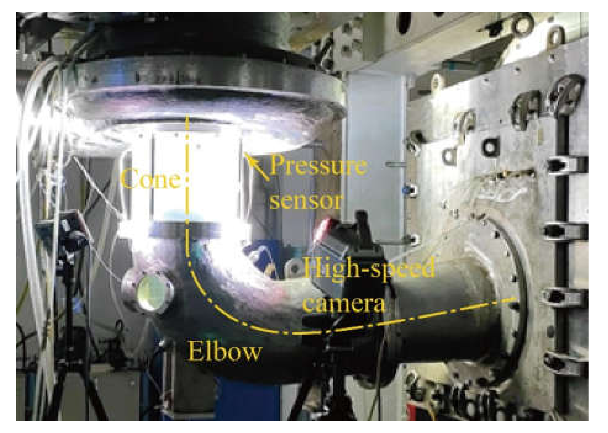
Experiments were carried out at the test facilities of the Kutateladze Institute of Thermophysics, Laboratory of Ecological Problems of Heat Power Industry, on a vertical experimental rig with the simplified turbine model (ST) with a Plexiglas draft tube cone (Figure 1), which provides optical access for different visualization techniques. The swirl generator designed to simulate flow in a Francis turbine operated at different discharge conditions is similar to the swirl generator designed at the Politehnica University of Timisoara, Romania [22]. The swirl intensity is varied by changing the two main parameters, i.e., the flow rate and the runner rotational speed. A detailed description of the experimental setup can be found in [19], where it is also shown that the simplified model can simulate flow distributions of a real Francis turbine to some extent. A sealed expansion tank with a free surface and a vacuum pump connected to it is installed in the upper part of the hydraulic test rig. This allows varying of the pressure level (dP) in the vortex chamber controlling the cavitation inception number. The water used in the experiments was degassed by heating and turbulizing the flow and then evacuating the released air with a vacuum pump from the top of the test rig. This procedure was carried out as long as the process of evacuating the released air led to a change in pressure.
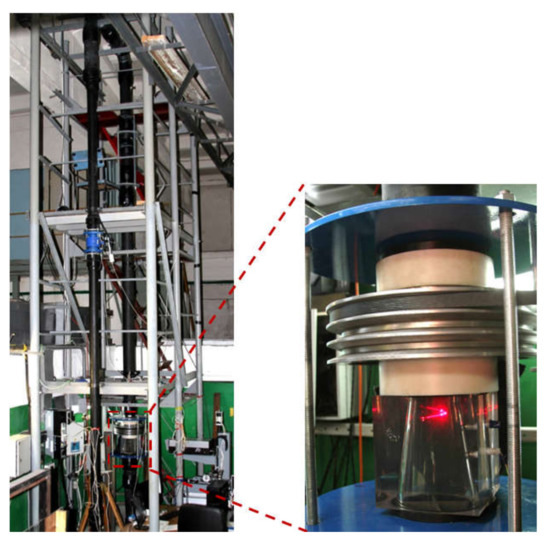
Figure 1.
Photo of the experimental setup. The main flow direction is downwards. The runner is rotated clockwise viewed from the top. Turbine runner rotational speed n is up to 3000 r/min. Maximum flow rate Q = 0.056 m3/s. Maximum Reynolds number .
The development of modern techniques and approaches for visualizing vortex flow, including computer graphics visualization using advanced methods based particularly on volume rendering of Eulerian fields, make a significant contribution to understanding the complex structure of the unsteady vortex flow [23]. However, vortex flow analysis can be carried out not only on the basis of velocity field data, but also using processing of high-speed imaging data. Vortex flow pattern was studied via a high-speed visualization system containing a pco.1200 hs camera at 820 fps frame rate and a system for flow illuminating with a powerful floodlight that allowed us to obtain contrast in the images. To achieve a high contrast image of the vaporous phase, an LED backlight source was placed opposite the camera behind the draft tube cone. With the selected lighting scheme, due to the scattering of light at the interface, the obtained images contained a uniform light background with darker areas corresponding to the vaporous cavities. We used image digital processing, which made it possible to identify and analyze the cavitation cavity based on high-speed visualization data. In the first step, the contours of cavities were determined by the binarization method. The algorithm includes image conversion to grayscale, contrast optimization, noise removal, and multi-stage edge detection based on Otsu’s double thresholding method. Assuming that the vaporous cavity is quasi-symmetric with respect to the axis of the draft tube, the image area was integrated over the angle. Based on the temporal realization of the vaporous cavity volume for each mode, spectrograms were computed using FFT. The temporal resolution was sufficient to resolve the most powerful of the cavitation cavity frequencies when applying fast Fourier transform (FFT) to the processed images. The first attempts to use this approach for flow analysis were presented in [24]. Below one can see the generalized Table 1 of studied operating conditions.

Table 1.
Studied operating conditions (ST).
2.2. Model Pump–Turbine
A 1:8.3 reduced scale pump–turbine runner (PT) with 7 blades was tested on the experimental platform of the hydraulic machinery at the Harbin Institute of Large Electrical Machinery (HILEM), see Figure 2.

Figure 2.
Draft tube section with pressure sensors on test rig in HILEM.
The installed capacity of the corresponding prototype pump–turbine is 50 MW, with a rated head of 97.7 m, a rated rotational speed of 300 r/min, and a specific speed r/min, where is its rated flow rate. Major parameters of the model pump–turbine are listed in Table 2. The closed-loop test rig has a maximum head of 80 m and a maximum discharge of 0.8 m3/s, and allows for accurate performance tests of the models with an accuracy of 0.2% in hydraulic efficiency measurements, in accordance with IEC Standards [25].
Table 2.
Major parameters of the model pump–turbine.
The measurements of the flow rate , the runner rotating speed , and the hydraulic head between the turbine inlet and at the draft tube outlet enable the determination of the unit speed and the unit flow rate corresponding to the tested operating points. The pressure level in the draft tube is regulated with a vacuum pump connected with the downstream reservoir and defined by the Thoma number , where is the net positive suction head
where is the pressure at downstream reservoir above the free surface level, is the vapor pressure, is the setting level of the machine with respect to the downstream reservoir, and is the flow velocity at the draft tube outlet. In the tests performed in this research, the experimental head is determined by the main pump and the electromotor connected to the model pump–turbine shaft, and the flow rate is regulated mainly via the guide vane opening. The draft tube has a transparent Plexiglas cone section, as shown in Figure 2.
By considering the velocity diagrams at the runner outlet, in which the axial flow velocity distribution is simplified as independent of the radial position, Favrel et al. [26] proposed an estimate of the swirl number characterizing the intensity of the swirling flow in terms of flow discharge and speed factors as
where and are the discharge factor and the unit flow rate in swirl-free conditions for the given speed factors and , respectively, at which the flow is theoretically axial. Although it is a simplified treatment in the calculation of , this definition is of practical importance since only operational factors of the units are needed. We thus adopt this method in the analysis of the flow characteristics in PT experiments.
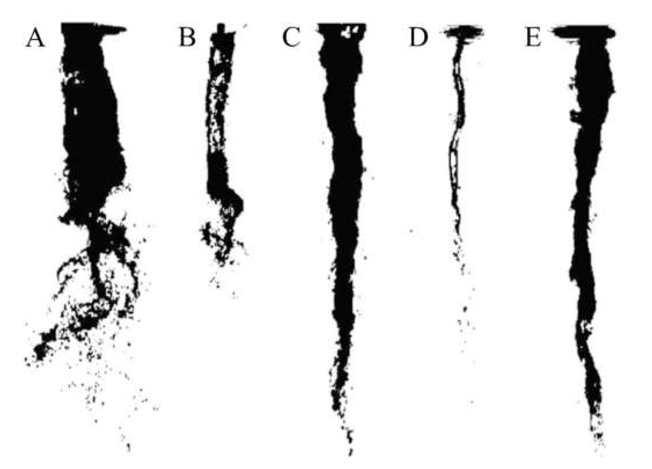
Figure 3 shows the Hill diagram of the model pump–turbine in () and () labelled by the guide vane opening , together with typical patterns of the cylindrical cavitating vortices in the draft tube at 5 tested conditions at . The swirl-free condition line for this particular unit was estimated by visual identification of the cavitation-free flows in the draft tube cone, and was approximated as a straight line in terms of and with the formula , as illustrated by the blue double-dotted line. Thus, the swirl number at a given working condition can be evaluated as
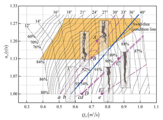
Figure 3.
Hill diagram in unit parameters with 5 isolines of the swirl number. The letters A–E indicate the location of the studied regimes on the hill diagram according to Table 3. a (); b ( ); c ( ); d ( ); and e ( ).
Images of the draft tube vortices were captured by a high-speed camera Phantom v9.1 at 1000 fps with a resolution of 1632 pixel × 1200 pixel. Pressure fluctuations in the pump–turbine were measured at a sampling rate of 4000 Hz by monitoring wall flush-mounted pressure sensors positioned in accordance with IEC standards [25]. A cylindrical cavitating vortex was observed in the swirl number range 0.1–0.5. Table 3 summarizes the studied operating conditions.
Table 3.
Studied operating conditions (PT).
Figure 4 demonstrates the cavitating vortex patterns for various pump–turbine operating conditions in which vortex ropes have a column-like shape and are more unstable for volume oscillation. However, Section 3.2 provides an analysis only for regimes A and C, in which the pressure pulsations in the draft tube cone were the largest.

3. Results and Analysis
3.1. Characteristics of ST
For high-speed visualization analysis, binarization of images was applied. A binary image obtained from a 2-D grayscale image was created by replacing all values above a globally determined threshold with 1 s and setting all other values to 0 s. Otsu’s method was used, which chooses the threshold value to minimize the intraclass variance of the threshold black and white pixels [27]. A 256-bin image histogram was calculated to compute Otsu’s threshold. The spiral part of the vortex could be cropped. After this procedure, the edges of the vortex rope are detected to calculate the local cross section areas of the cavity, as exemplified in Figure 5 for condition 5 (n = 910 r/min and Q = 0.031 m3/s) described in Section 2.1. The fluctuating part of the cavitation volume oscillation can be accurately estimated by integration.
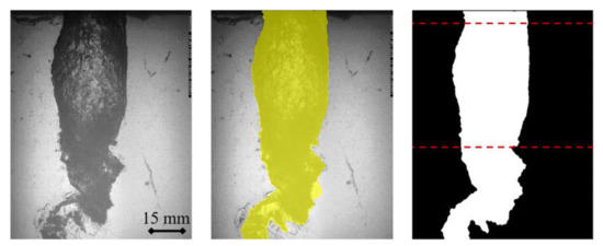
Figure 5.
Example of image processing. Raw, masked, and binarized images. Condition 5 (n = 910 r/min and Q = 0.031 m3/s).
Below in Figure 6, one can see the time evolution of the cavity during 3 s and the corresponding signals of calculated and filtered volume. The series of images are obtained from high-speed flow visualization with a shooting frequency of 850 fps. The selected images cover a full oscillation cycle and show the different stages of the oscillation of the vaporous cavity at a low-frequency. One can see that fragment (d) has a significantly larger cavity volume compared with Figure 6a. The spiral breakdown point position moves upstream and then downstream making periodic oscillations, such motion is characterized by local changes in the flow swirl parameter. As the vortex cavity volume increases, the local hydrodynamic resistance increases too, which is accompanied by pulsations of the liquid column and its effects on the runner of the model turbine. Moreover, as the diameter of the vaporous cavity increases, the local section decreases and the local parameter of the flow swirling increases. The study of the mechanism of self-excited oscillations is a relevant issue in the safe operation of natural hydraulic units.
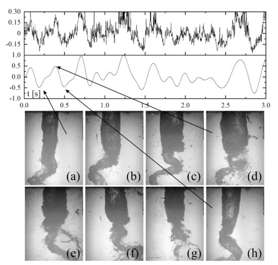
Figure 6.
Time evolution of vortex volume oscillation. Condition 5 (n = 910 r/min and Q = 0.031 m3/s). (a–h) indicate different vortex stages during one oscillation cycle.
Similar fluctuations in the position of the vortex breakdown in the simplified geometry of the draft tube (Venturi cone) were observed in [28]. The authors claim that synchronous pressure pulsations are identified as the product of self-excited oscillations of vortex breakdown location.
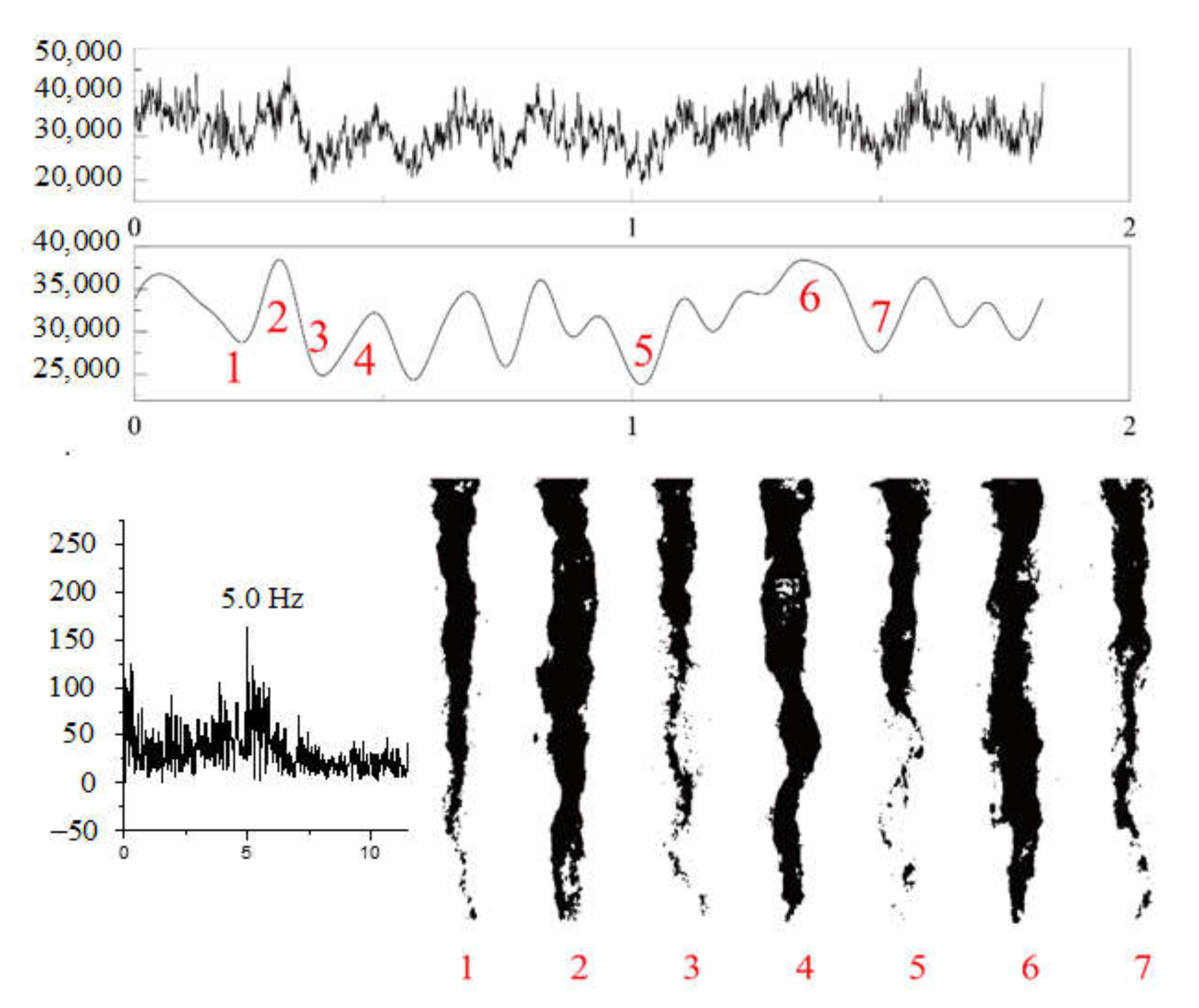
The typical FFT of volume oscillation as demonstrated for condition 5 is shown below in Figure 7 for condition 3 for one image set. Condition 3 is chosen as an example because it covers the largest range of frequencies that appear. Whereas for condition 5, volume fluctuations at low frequencies predominate in the spectrum.

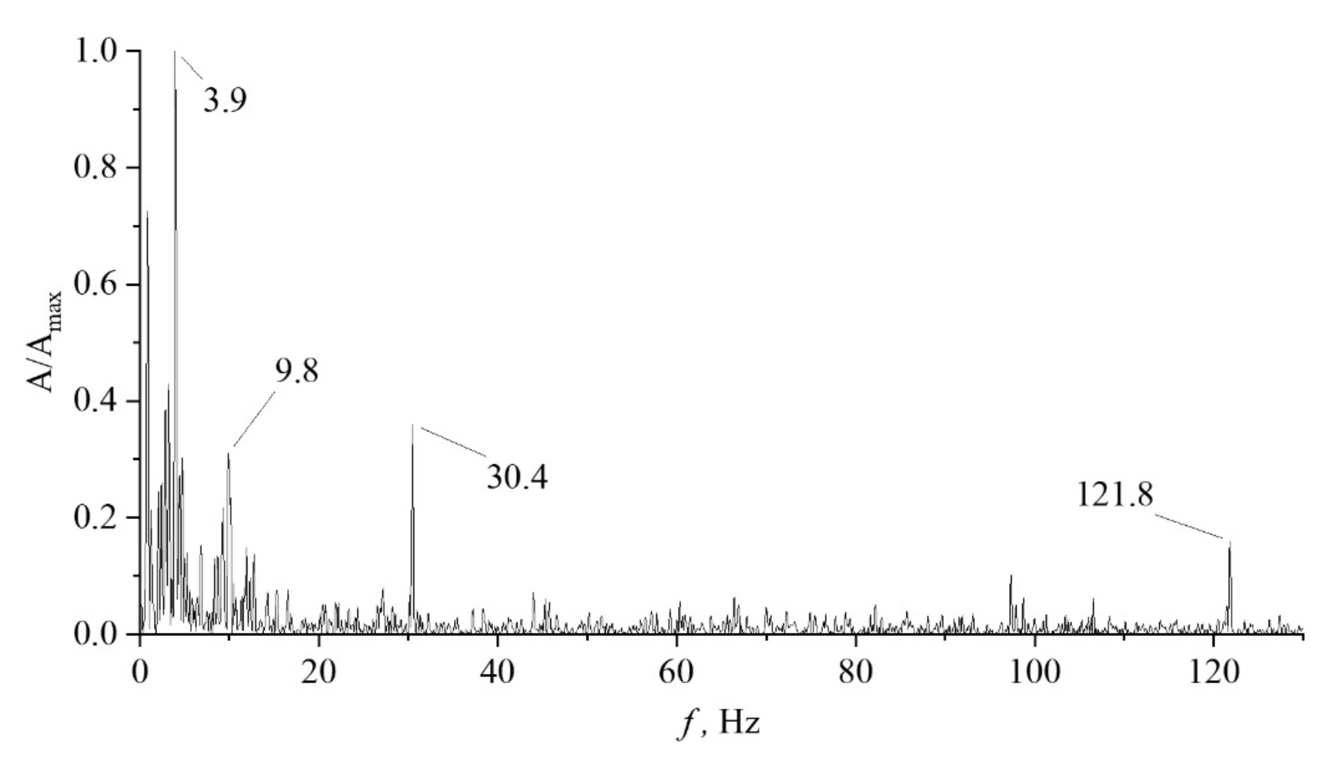
Figure 7.
Fourier spectrum of estimated vortex rope volume. Condition 3 (n = 860 r/min and Q = 0.031 m3/s).
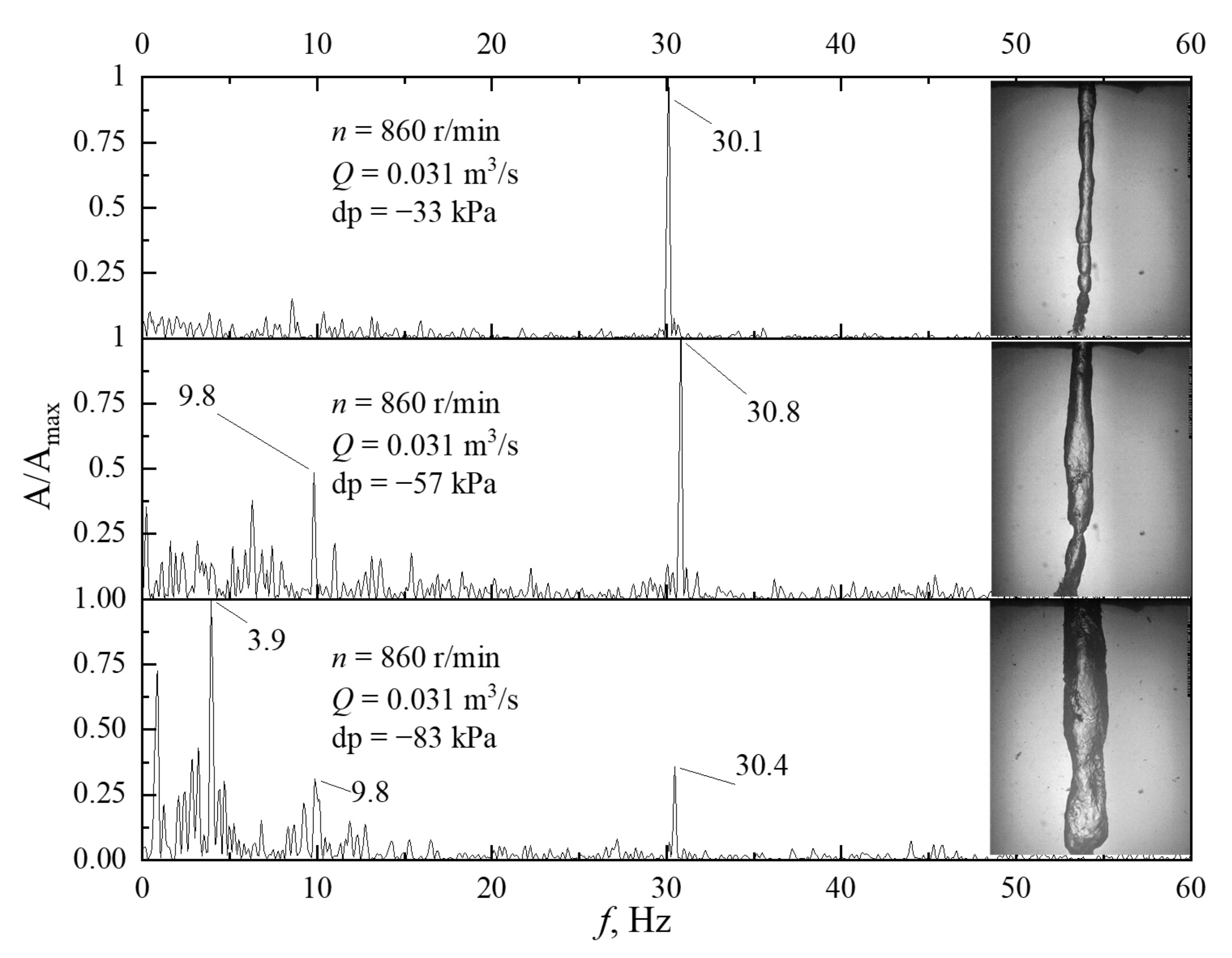
Figure 7 demonstrates the normalized power spectral density of cavity volume oscillations for condition 3 (n = 860 r/min and Q = 0.031 m3/s), but the same or close frequencies were found at other studied conditions. It can be seen that several frequencies dominate the spectrum: 3.9 Hz, 9.8 Hz, 30.4 Hz, and 121.8 Hz. (f/n~0.27, 0.68, 2.12, 8.44, respectively). By decomposing the original signal at these frequencies, it is possible to obtain images of the change in volume at each frequency. The frequency f of 3.9 Hz (f/n~0.27) is dominant and probably corresponds to a low-frequency “breathing” cavity motion with the highest amplitude. The volumetric change can reach 80–90%. Other frequencies, 9.8 and 30.4, are presumably high-frequency modulation of the low-frequency oscillations of the volume (about 10% of volume change), and the frequency 121.8 corresponds to waves propagating along the vortex, resulting in the formation of small local constriction reducing the cavity volume. Two different cases were considered: cavitation condition variation for the same working point (Figure 8) and swirl number variation at the same flow rate (Figure 9). A series of experiments were carried out at a fixed flow rate and runner rotational speed and a variation of the additional vacuum in the tank connected to the hydraulic test rig. Figure 8 shows three spectrograms corresponding to different pressure conditions. The dP value in the figures corresponds to the additional vacuum in the working section relative to the atmospheric pressure without considering the liquid head. It can be seen that, with a smaller pressure drop, dP = −33 kPa, the vortex cavity has a much smaller volume. Analyzing the spectral characteristics, it can be found that large-scale volumetric pulsations at a low frequency of 3.9 Hz disappear, but pulsations at a frequency of about 30 Hz remain and dominate.

Figure 8.
Pressure spectrums and flow patterns for different dP cases at n = 860 r/min and Q = 0.031 m3/s ().

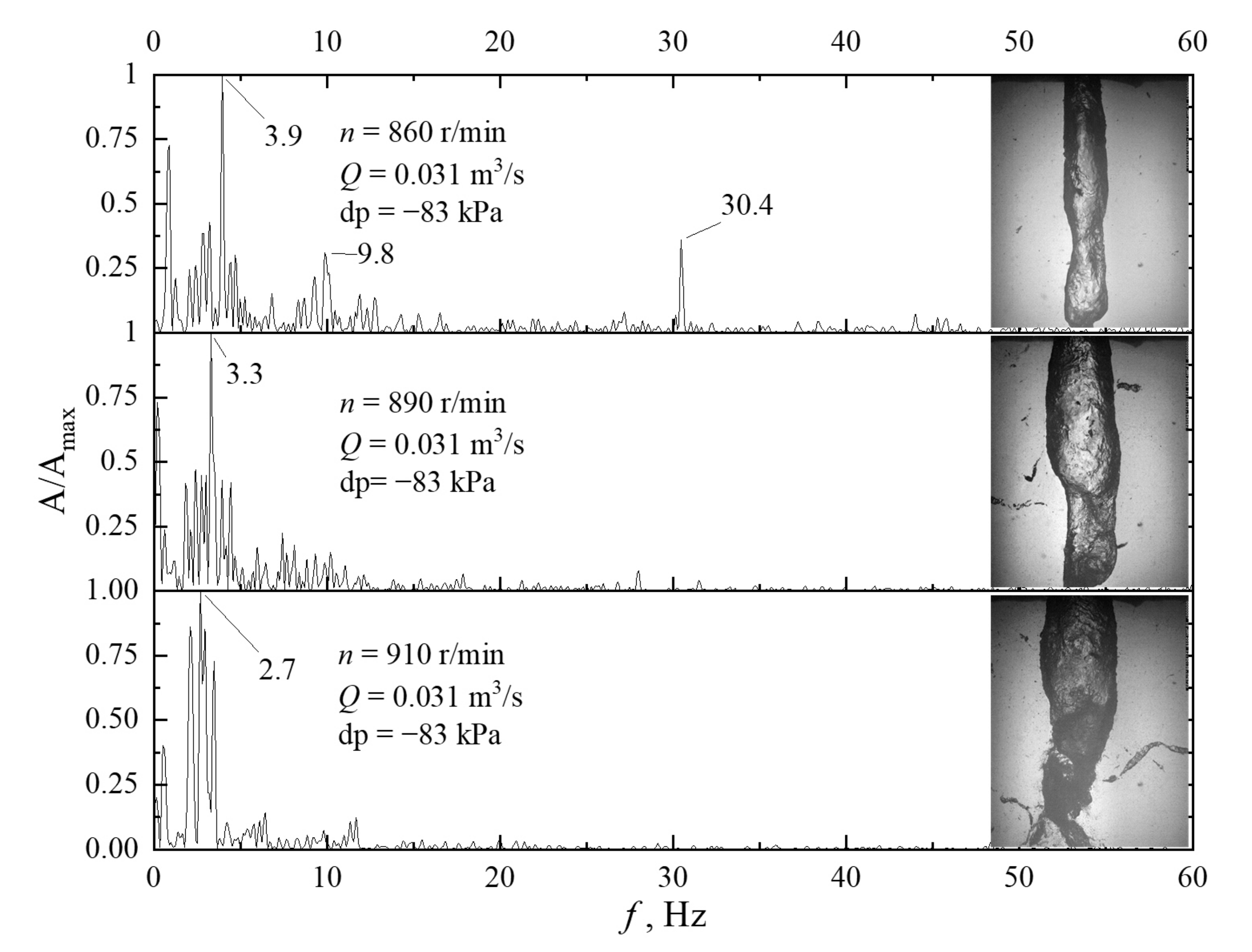
Figure 9.
Pressure spectrums and flow patterns at dP = −83 kPa for respectively (a) n = 860 r/min and Q = 0.031 m3/s (); (b) n = 890 r/min and Q = 0.031 m3/s ( ); and (c) n = 910 r/min and Q = 0.031 m3/s ( ).
The presence of a distinguished peak in the spectrum only at sufficient rarefaction confirms the hypothesis about the cavitation nature of the occurrence of cavity volume oscillations. Having reached the conditions when low-frequency oscillations of the vapor cavity are observed by creating an additional rarefaction, we start to vary the intensity of the flow swirl.
Comparing the model pump–turbine, the swirl number used here can be estimated using equation
that was previously verified in work [19] and was originally proposed in work [26]. Thus, S = 0.22 for n = 860 r/min and Q = 0.031 m3/s. The swirl was varied in the range S = 0.2–0.4. At S > 0.4, the vortex rope began to acquire a classical spiral shape.
With an increase in the swirl parameter, the frequency of self-excited oscillations decreases. The stagnation point moves upward which forms a cavity with a larger radius and a shorter length.
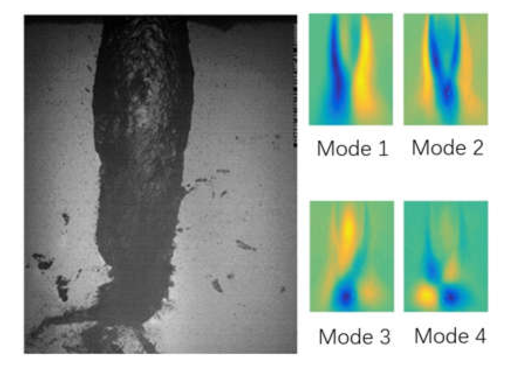
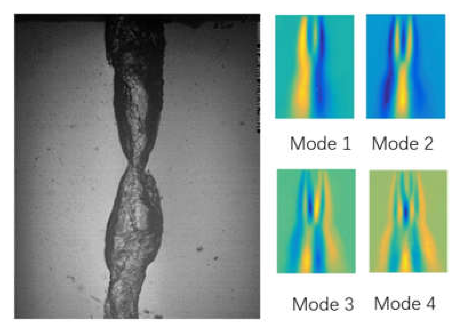
Some information can be obtained from decomposing the visualization into orthogonal modes. A snapshot proper orthogonal decomposition (POD) technique is used to identify different modes of the oscillations of the cavitating cylindrical vortices. This method was firstly proposed by Sirovich [29] to reduce the calculation time, and has been employed in the analysis of cavitation flows [30]. By applying this technique to decompose the sequences of high-speed grey-scale images of cavitating vortices, the most energetic coherent vapor structures associated to each oscillating mode can be detected. In Figure 10 and Figure 11 one can see the four most energetic POD modes. The mode associated with the volumetric change is axisymmetric (mode 2). The modes representing the precession motion of the vortex are not axisymmetric. The 4th POD mode with a narrow symmetric region can correspond to traveling waves along the cavitation cavity, which look like a local narrowing of the cavity on high-speed imaging. The first POD modes also confirm the different nature of the frequencies in the spectrum obtained from the area analysis of the binarized images.

Figure 10.
POD modes of vapor cavity structures at n = 910 r/min, Q = 0.031 m3/s, and dP = −83 kPa.

Figure 11.
POD modes of vapor cavity structures at n = 860 r/min, Q = 0.031 m3/s, and dP = −83 kPa.
3.2. Characteristics of PT
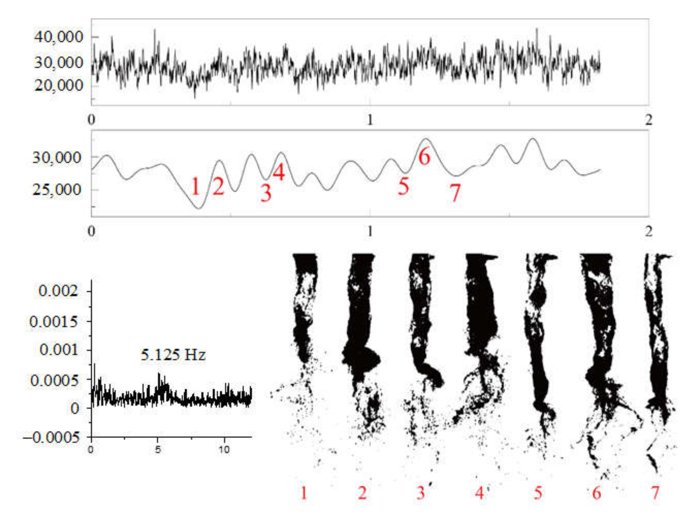
For the pump–turbine, the image processing procedure was the same as for the simplified geometry. Since the PT was equipped with a pressure sensor in the draft tube wall, it was possible to confirm that a visual change in the volume of the cavity is also accompanied by pressure pulsations. To distinguish the axisymmetric cavitation cavity form, a sequential filtering and binarization procedure was also used. In total, five different operating points were considered (Table 3), marked on the map with circles in Figure 3. The values of the frequencies obtained using FFT are listed in the last column of Table 3. It should be noted that in all the mentioned operating conditions, at the end of the axisymmetric cavitation cavity, there is a spiral vortex breakdown part, which is also a source of pressure fluctuations (asynchronous). However, since the pressure sensor is located in the region of a symmetrical cavity, we register precisely synchronous pressure fluctuations. Below are several characteristic modes, where the pulsations of the volume of the vaporous cavity are the largest. The pressure signals from the sensor shown in Figure 2 are presented below to provide comparisons against videos of the evolution of cavitating vortices in the draft tube (Figure 12 and Figure 13).

Figure 12.
Pressure fluctuation and flow pattern for operating condition A.

Figure 13.
Pressure fluctuation and flow pattern for operating condition C.
Visually, the vaporous structures at operating conditions A and C are qualitatively similar and correlate well with operating condition 5 in the ST. Compared with the pulsation spectra obtained for a simplified turbine, there are no peaks with a higher frequency in the pressure pulsation spectrum for the pump–turbine in the studied modes. It can be concluded that small-scale volumetric pulsations at higher frequencies (associated, for example, with the presence of low-amplitude waves traveling along the vortex cavity) do not affect the flow path and are of no significant interest from the point of view of the operational safety of hydraulic units.
4. Theoretical Approach
4.1. Basic Principle
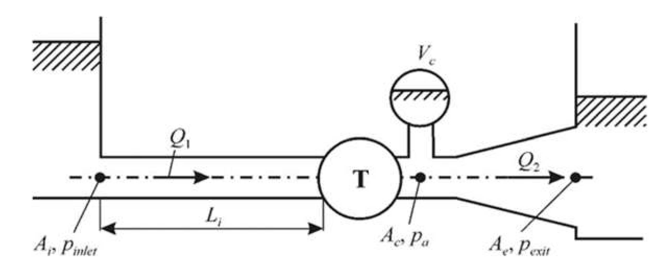
Using the geometry of the pump–turbine flow path (Figure 14), the one-dimensional model describing the oscillations of cavitation bubble arising behind the hydraulic turbine runner proposed is adopted and improved. The approach for the instability analysis proposed by Chen et al. [13] is based on the system of two governing equations. The first equation is essentially a continuity equation. It presents the relationship between the flow rates in the penstock, , and in the draft tube,
Figure 14.
Scheme of the hydraulic parts of the turbine.
The second equation is the Bernoulli equation, it represents the relationship between the pressure at the system inlet, , and the exit pressure,
Here, the indices and correspond to inlet and exit cross sections and index relates to the cavity; is the liquid density; is the effective length of the draft tube (DT); ( is the area of DT cross-section as a function of the curvilinear coordinate ); is the diffusor factor; is the DT loss factor; and is the turbine loss factor. The coefficient in Equation (5) is the pressure coefficient responsible for the swirl effect, which will be discussed later. is the angle of inclination of the runner blade at the exit; is the area of the outlet cross section of the runner; and is the peripheral velocity at the exit from the runner; thus, the characteristic circumferential flow velocity here is
The cavitation compliance reflects the rate of cavity volume variation versus the pressure change. In [13], it is evaluated from the condition that the frequency given by the equation equals 0.16 times the runner rotational frequency, . In the present paper, we evaluate from some physical principles.
For the stability analysis, the flow rates are represented as , , and oscillations are assumed to be small, i.e., and . It is obvious that mean flow rates and are equal to each other, . Further, we represent the oscillatory functions and in the form and , respectively, where is the imaginary unit. Substituting these expressions into Equations (5) and (6), one obtains a system of homogeneous linear equations with respect to and . Equating the determinant of the matrix of this system of linear equations to zero, we obtain the characteristic equation
Here, the coefficients are as follows
Equation (7) is an equation of the third order with respect to with real coefficients. Its roots in the general case are complex and one can obtain a complex frequency . The real part, , corresponds to the frequency, and the imaginary part, , to the damping/amplification rate (decrement/increment) of the perturbances. If we have one solution , then is the second solution. Solutions and are essentially the same solution with the same frequency and decrement. The real part of the third solution is equal to zero, i.e., , and this solution does not represent unstable modes. An unstable solution arises when is negative.
4.2. Pressure Distribution Calculation behind the Runner
To study the cavitating flows in the draft tube, let us consider the approach proposed by Kuibin et al. [14]. The authors considered three models of axi-symmetrical vortices with helical vortex lines (with the vorticity distributions corresponding to Rankine, Lamb, and Scully vortices, respectively) introduced in [31,32,33]. In these models, tangential () and axial () velocity components were represented through a single function being an integral from the axial component of vorticity as
Here, is the total intensity of the vortex, is the pitch of helical lines, and is the value of axial velocity at the vortex axis. The pressure was found by integration
where is the pressure at the vortex axis. As was shown in [31,32,33], the vortex with Rankine-type vorticity distribution is most convenient due to simple analytical representation of the vorticity field, but it is far from real vortices. The Lamb’s type is proper for description of the laminar vortices. The third one is a model with vorticity distributions of the Scully type,
which gives us the opportunity to describe turbulent vortices. Here, is the size of the vortex. For this model we obtain
In a liquid, when the pressure becomes less than the liquid vapor pressure, a cavitation area arises in the near-axis zone of the vortex. In the model proposed in [14,15], the cavity of constant radius along the vortex was considered with a boundary coinciding with the isosurface of pressure equal to the liquid vapor pressure, i.e., the pressure in the cavity . Therefore, we can obtain the mean pressure for the cross section of the draft tube of radius
At the same time, the mean pressure over the DT entrance cross section can be expressed through the Bernoulli’s integral
Here, is the tail water pressure that is equal to the atmospheric one, is the difference of heights between the inlet cross section and the tail water level, is the velocity averaged over the cross section, and is the gravity acceleration. If we equate from (8) and from (13), we obtain the equation for determination of the cavity radius .
In a paper by Chen et al. [13], the pressure in the vortex core was considered as linked with the ambient pressure and the peripheral swirl velocity behind the runner, i.e.,
In the case under consideration, we find
Finally, as the volume of the cavity in the model , Equation (12) allows to find the cavitation compliance
4.3. Simulation of the Cavity Oscillations
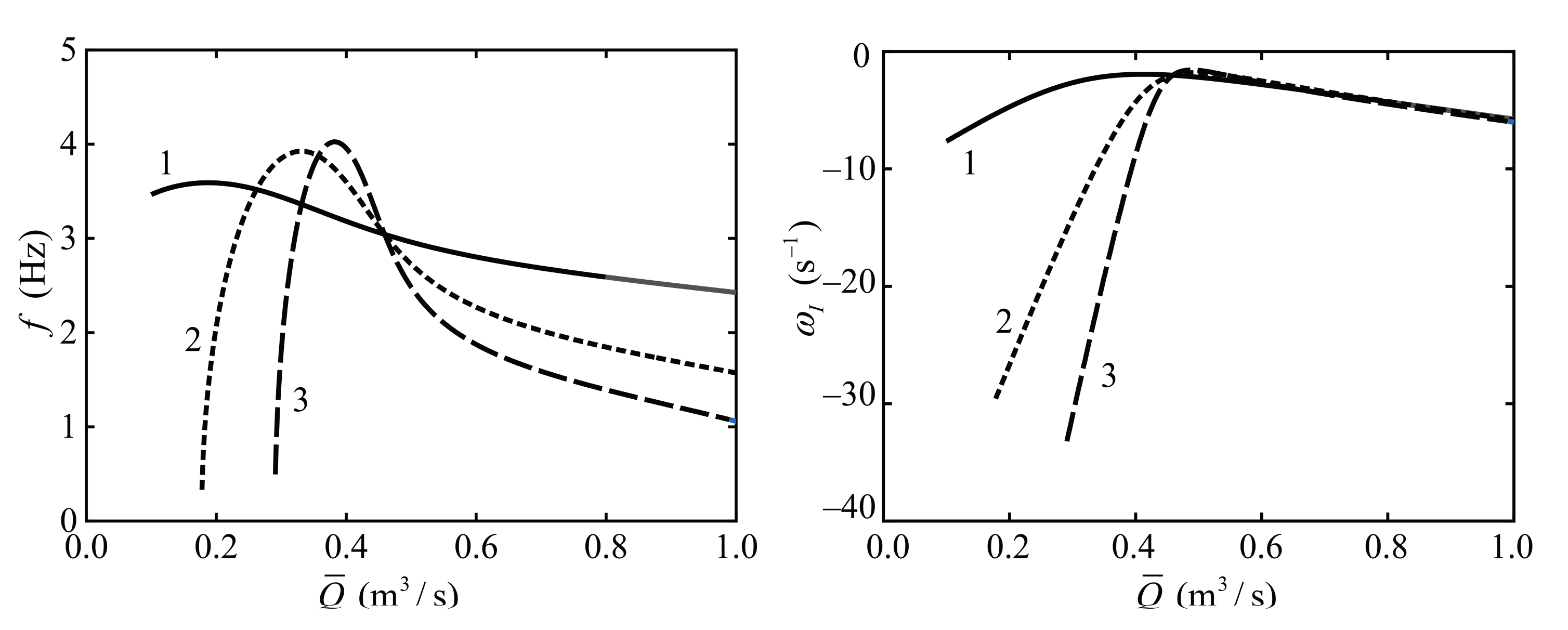
In Figure 15, the plots of frequencies and increments of the cavity oscillations are presented. The calculation in accordance with Equation (7) for parameters corresponding to experimental data presented above for operating condition B for PT, cavitation compliance C evaluated by the method recommended in [13], and three fixed values of α = 1, 5, and 10. At this condition (see Figure 3), we have Q11 = 0.702 m3/s (Q = 0.316 m3/s) and a frequency with maximum amplitude f = 5.75 Hz. Calculation by the model proposed in [13] predicts unstable perturbations values with lower frequencies 3.4 Hz, 3.9 Hz, and 2.8 Hz for α = 1, 5, and 10, respectively.
Figure 15.
Frequencies (left) and increments (right) of the cavity oscillations. 1. α = 1; 2. α = 5; and 3. α = 10. C = 1.84 × 10⁻⁷ m4 s2/kg is evaluated in accordance with recommendations from [13].
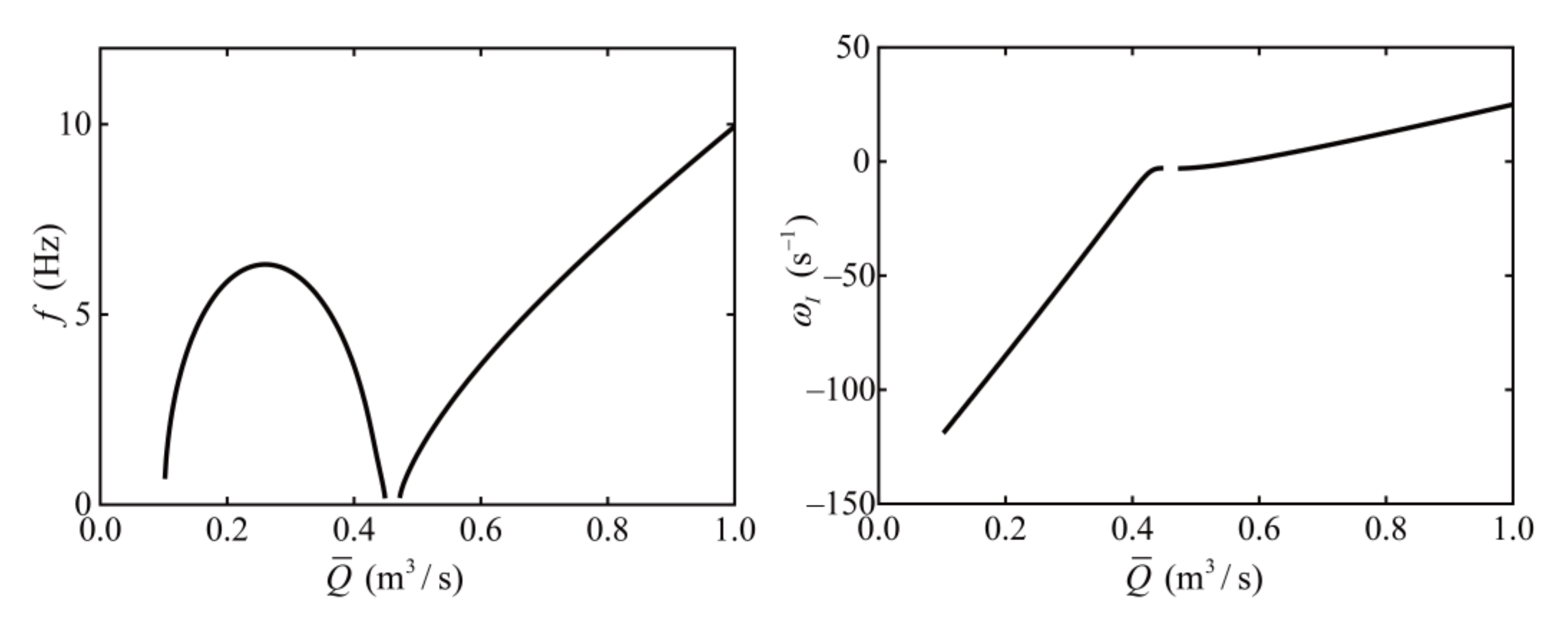
For the model developed in [14,15] with coefficient dependent on the model parameters (see Equation (15)) and cavitation compliance flow rate determined by Equation (16), we can find parameters of the vortex and cavity providing the frequency found in the experiment. For example, at = 0.16 and = 0.59 we obtain unstable mode with frequency 5.75 Hz. The dependencies of cavity oscillations frequency and the damping rate on the flow rate for these parameters of the vortex are shown in Figure 16. There are two diapasons of unstable disturbances: at and . At the periodical solutions of Equation (7) are absent. At the oscillations become damping.

Figure 16.
Frequencies (left) and increments (right) of the cavity oscillations. Parameter α is calculated by Equation (15) and C is calculated by Equation (16).
Finally, in Figure 17 we collect a plot of vortex parameters providing prediction of unsteady cavity oscillations for all five operating conditions studied in the experiments.
Figure 17.
Relative vortex size vs relative size of cavity providing the frequencies of unstable cavity oscillations found in the current experiments. The characters A–E correspond to the experimental operating conditions of PT (see Figure 3).
5. Conclusions
Using the methods of experimental modeling in a simplified turbine model, a similar flow pattern was reproduced qualitatively as observed in a draft tube of a Francis turbine operated under full-load conditions. This study attempts to correlate these observations with a full-load surge phenomenon in a simplified Francis turbine (ST). The phenomenon of self-excited cavitating vortex volume oscillation has been reproduced in the simplified turbine model. The flow patterns look similar to the flow pattern as observed in a draft tube of Francis turbine operated under full-load conditions. Large-scale cavitation cavities oscillate significantly in time, which is an additional source of unsteady flow rate and pressure pulsations in the hydrodynamic path. Detailed investigation of flow patterns over time were performed via a high-speed visualization technique and subsequent digital image analysis. Using FFT, four different oscillation frequency ranges for ST, f~3 Hz, 10 Hz, 30 Hz, and 120 Hz at Q = 0.031 m3/s, were revealed. A similar flow pattern was observed in our experiments on a reduced scale pump–turbine (PT) in HILEM where five operating conditions were also considered. It is shown that the cavitation pulsating cavity can be observed not only in the full-load mode, but on both sides of the BEP with full and partial load. The frequencies corresponding to large-scale fluctuations in the volume of the cavitation cavity are in the range of 5–5.75 Hz (f/n~5–5.5). The reproducibility of the phenomenon on a model installation, as well as on a pump–turbine, confirms that this phenomenon accompanies a wide class of hydraulic turbines of various geometries. Based on the geometry of the pump–turbine and the frequency values associated with the oscillations of the vaporous cavity, an analytical approach was used to provide a prediction of unsteady cavity oscillations for all five operating conditions studied in the experiments. The one-dimensional model describing the oscillations of cavitation bubbles arising behind the hydro turbine runner proposed by Chen et al. [13] and developed by Kuibin et al. [15] was adopted for description of the current experiments. It is shown that for a certain ratio between relative vortex size and relative size of cavity, which are free parameters in the analytical model, it is possible to predict the frequency of self-excited pulsations.
The obtained data will be useful for further tuning a one-dimensional hydro-acoustic model describing the cavitation phenomenon with better precision.
Author Contributions
Conceptualization, S.S. and Z.Z.; methodology, S.S., Z.Z., and P.K.; validation, M.T. and S.L.; formal analysis, S.S., Z.Z., and P.K.; investigation, S.S., M.T., Z.Z., and P.K.; data curation, S.S., Z.Z., and S.L.; writing—original draft preparation, S.S., Z.Z., and P.K.; writing—review and editing, S.S. and Z.Z.; supervision, S.S. and Z.Z.; project administration, P.K., Z.Z., and S.L.; funding acquisition, P.K. and Z.Z. All authors have read and agreed to the published version of the manuscript.
Funding
The study of the simplified turbine (ST) and development of an analytical approach were supported by a grant from the Russian Science Foundation (project no. 21-79-10080), the study of the pump–turbine (PT) was supported by the National Natural Science Foundation of China (no. 52076120 and no. 52079066), the open Fund of State Key Laboratory of Eco-hydraulics in Northwest Arid Region (no. 2018KFKT-10), the State Key Laboratory of Hydroscience and Engineering (2019-KY-04, sklhse-2019-E-02 and sklhse-2020-E-03), and the Creative Seed Fund of Shanxi Research Institute for Clean Energy, Tsinghua University.
Institutional Review Board Statement
Not applicable.
Informed Consent Statement
Not applicable.
Data Availability Statement
Not applicable.
Conflicts of Interest
The authors declare that they have no conflict of interest.
References
- Favrel, A.; Müller, A.; Landry, C.; Yamamoto, K.; Avellan, F. LDV survey of cavitation and resonance effect on the precessing vortex rope dynamics in the draft tube of Francis turbines. Exp. Fluids 2016, 57, 168. [Google Scholar] [CrossRef]
- Lu, G.; Zuo, Z.; Sun, Y.; Liu, D.; Tsujimoto, Y.; Liu, S. Experimental evidence of cavitation influences on the positive slope on the pump performance curve of a low specific speed model pump-turbine. Renew. Energy 2017, 113, 1539–1550. [Google Scholar] [CrossRef]
- Alligne, S.; Nicolet, C.; Tsujimoto, Y.; Avellan, F. Cavitation surge modelling in Francis turbine draft tube. J. Hydraul. Res. 2014, 52, 399–411. [Google Scholar] [CrossRef]
- Li, D.; Sun, Y.; Zuo, Z.; Liu, S.; Wang, H.; Li, Z. Analysis of Pressure Fluctuations in a Prototype Pump-Turbine with Different Numbers of Runner Blades in Turbine Mode. Energies 2018, 11, 1474. [Google Scholar] [CrossRef] [Green Version]
- Rheingans, W.J. Power swings in hydroelectric power plants. Trans. ASME 1940, 62, 171–184. [Google Scholar]
- Valentín, D.; Presas, A.; Egusquiza, E.; Valero, C.; Egusquiza, M.; Bossio, M. Power Swing Generated in Francis Turbines by Part Load and Overload Instabilities. Energies 2017, 10, 2124. [Google Scholar] [CrossRef] [Green Version]
- Müller, A.; Favrel, A.; Landry, C.; Yamamoto, K.; Avellan, F. Experimental Hydro-Mechanical Characterization of Full Load Pressure Surge in Francis Turbines. J. Phys. Conf. Ser. 2017, 813, 12018. [Google Scholar] [CrossRef] [Green Version]
- Braisted, D.M.; Brennen, C.E. Auto-Oscillation of Cavitating Inducers. In Proceedings of the Polyphase Flow and Transport Technology, San Francisco, CA, USA, 13–15 August 1980; pp. 157–166. [Google Scholar]
- Nishi, M.; Kubota, T.; Matsunaga, S.; Senoo, Y. Study on swirl flow and surge in an elbow type draft tube. In Proceedings of the 10th IAHR Symposium on Hydraulic Machinery and Cavitation, Tokyo, Japan, 9–11 September 1980; Volume 1, p. 557. [Google Scholar]
- Tsujimoto, Y.; Kamijo, K.; Yoshida, Y. Theoretical analysis of rotating cavitation in rocket pump inducers. In Proceedings of the 28th Joint Propulsion Conference and Exhibit, Nashville, TN, USA, 6–8 July 1992; American Institute of Aeronautics and Astronautics: Reston, VA, USA, 1992; Volume 115, pp. 135–141. [Google Scholar]
- Otsuka, S.; Tsujimoto, Y.; Kamijo, K.; Furuya, O. Frequency Dependence of Mass Flow Gain Factor and Cavitation Compliance of Cavitating Inducers. J. Fluids Eng. 1996, 118, 400–408. [Google Scholar] [CrossRef]
- Streeter, V.L. Transient Cavitating Pipe Flow. J. Hydraul. Eng. 1983, 109, 1407–1423. [Google Scholar] [CrossRef]
- Chen, C.; Nicolet, C.; Yonezawa, K.; Farhat, M.; Avellan, F.; Tsujimoto, Y. One-Dimensional Analysis of Full Load Draft Tube Surge. J. Fluids Eng. 2008, 130, 041106. [Google Scholar] [CrossRef]
- Kuibin, P.A.; Pylev, I.M.; Zakharov, A.V. Two-phase models development for description of vortex-induced pulsation in Francis turbine. IOP Conf. Ser. Earth Environ. Sci. 2012, 15, 022001. [Google Scholar] [CrossRef]
- Kuibin, P.A.; Zakharov, A.V. On low-frequency unsteady phenomena caused by cavitation in hydroturbines. IOP Conf. Ser. Earth Environ. Sci. 2019, 288, 012100. [Google Scholar] [CrossRef]
- Müller, A.; Favrel, A.; Landry, C.; Avellan, F. Fluid–structure interaction mechanisms leading to dangerous power swings in Francis turbines at full load. J. Fluids Struct. 2017, 69, 56–71. [Google Scholar] [CrossRef]
- Müller, A.; Favrel, A.; Landry, C.; Yamamoto, K.; Avellan, F. On the physical mechanisms governing self-excited pressure surge in Francis turbines. IOP Conf. Ser. Earth Environ. Sci. 2014, 22, 32034. [Google Scholar] [CrossRef] [Green Version]
- Müller, A.; Yamamoto, K.; Alligné, S.; Yonezawa, K.; Tsujimoto, Y.; Avellan, F. Measurement of the Self-Oscillating Vortex Rope Dynamics for Hydroacoustic Stability Analysis. J. Fluids Eng. 2015, 138, 021206. [Google Scholar] [CrossRef]
- Skripkin, S.; Tsoy, M.; Kuibin, P.; Shtork, S. Swirling flow in a hydraulic turbine discharge cone at different speeds and discharge conditions. Exp. Therm. Fluid Sci. 2019, 100, 349–359. [Google Scholar] [CrossRef]
- Li, D.; Chang, H.; Zuo, Z.; Wang, H.; Li, Z.; Wei, X. Experimental investigation of hysteresis on pump performance characteristics of a model pump-turbine with different guide vane openings. Renew. Energy 2020, 149, 652–663. [Google Scholar] [CrossRef]
- Szakal, R.-A.; Doman, A.; Muntean, S. Influence of the Reshaped Elbow on the Unsteady Pressure Field in a Simplified Geometry of the Draft Tube. Energies 2021, 14, 1393. [Google Scholar] [CrossRef]
- Bosioc, A.I.; Susan-Resiga, R.; Muntean, S.; Tanasa, C. Unsteady Pressure Analysis of a Swirling Flow With Vortex Rope and Axial Water Injection in a Discharge Cone. J. Fluids Eng. 2012, 134, 081104. [Google Scholar] [CrossRef]
- Urban, O.; Kurková, M.; Rudolf, P. Application of Computer Graphics Flow Visualization Methods in Vortex Rope Investigations. Energies 2021, 14, 623. [Google Scholar] [CrossRef]
- Skripkin, S.G.; Tsoy, M.A.; Kuibin, P.A.; Zuo, Z.; Liu, S. High speed visualization of self-oscillation of axisymmetric cavitating cavity in a square vortex chamber. J. Phys. Conf. Ser. 2019, 1421, 012029. [Google Scholar] [CrossRef] [Green Version]
- IEC 60193-6; Hydraulic Turbines, Storage Pumps and Pump-Turbines; International Commission: Geneva, Switzerland, 1999.
- Favrel, A.; Gomes Pereira Junior, J.; Landry, C.; Müller, A.; Nicolet, C.; Avellan, F. New insight in Francis turbine cavitation vortex rope: Role of the runner outlet flow swirl number. J. Hydraul. Res. 2018, 56, 367–379. [Google Scholar] [CrossRef]
- Otsu, N. A Threshold Selection Method from Gray-Level Histograms. IEEE Trans. Syst. Man. Cybern. 1979, 9, 62–66. [Google Scholar] [CrossRef] [Green Version]
- Khozaei, M.H.; Favrel, A.; Miyagawa, K. On the generation mechanisms of low-frequency synchronous pressure pulsations in a simplified draft-tube cone. Int. J. Heat Fluid Flow 2022, 93, 8912. [Google Scholar] [CrossRef]
- Sirovich, L. Turbulence and the dynamics of coherent structures. I. Coherent structures. Q. Appl. Math. 1987, 45, 561–571. [Google Scholar] [CrossRef] [Green Version]
- Danlos, A.; Ravelet, F.; Coutier-Delgosha, O.; Bakir, F. Cavitation regime detection through Proper Orthogonal Decomposition: Dynamics analysis of the sheet cavity on a grooved convergent-divergent nozzle. Int. J. Heat Fluid Flow 2014, 47, 9–20. [Google Scholar] [CrossRef] [Green Version]
- Kuibin, P.; Okulov, V. One-dimensional solutions for a flow with a helical symmetry. Thermophys. Aeromechanics 1996, 3, 335–339. [Google Scholar]
- Alekseenko, S.V.; Kuibin, P.A.; Okulov, V.L.; Shtork, S.I. Helical vortices in swirl flow. J. Fluid Mech. 1999, 382, 195–243. [Google Scholar] [CrossRef]
- Alekseenko, S.V.; Kuibin, P.A.; Okulov, V.L. Theory of Concentrated Vortices: An Introduction; Springer: Berlin/Heidelberg, Germany, 2007; ISBN 9783540733751. [Google Scholar]


Publisher’s Note: MDPI stays neutral with regard to jurisdictional claims in published maps and institutional affiliations. |
© 2022 by the authors. Licensee MDPI, Basel, Switzerland. This article is an open access article distributed under the terms and conditions of the Creative Commons Attribution (CC BY) license (https://creativecommons.org/licenses/by/4.0/).