Abstract
Road lighting uniformity is an essential lighting quality parameter for motorists and pedestrians and varies with lighting design parameters. Increased road lighting uniformity may result in benefits, such as increased reassurance and perceived safety for pedestrians or an increased overall visual perception. However, no previous study has investigated how road lighting uniformity varies with lighting design scenarios or how the uniformity of various lighting design scenarios affects other essential parameters, such as energy performance and obtrusive light. This study aimed to investigate: (I) how uniformity varies with different road lighting design scenarios, and (II) how uniformity correlates with energy performance and risk for increasing spill light. The study is limited to pedestrian roads. We performed photometric calculations in ReluxDesktop for more than 1.5 million cases with single-sided pole arrangements and for various geometries of road width, pole distance, pole height, overhang, and luminaire tilt. The results were analyzed with a set of five relevant metrics that were calculated and analyzed together with uniformity. For the evaluation, we used the minimum luminaire power needed to achieve an average illuminance of 10 lx, the power density indicator (DP), edge illuminance ratio (REI), and we introduced two new indicators for spill light on the ground in the border areas: the extended edge illuminance ratio (extended REI) and the spill flux ratio (RSF). The results show that increased uniformity levels may significantly increase energy consumption and spill light, but that both these impacts can be relatively controlled if uniformity is kept under certain limits. The investigated cases also demonstrated that improper lighting planning significantly increases adverse effects, such as spill light.
1. Introduction
Road lighting facilitates human usage of the exterior environment and is a significant aspect of sustainable urban development because it allows humans to have an active lifestyle in darkness and to engage in activities such as traveling, exercise, shopping, relaxing, working, or playing. The purpose of road lighting is to enable safe transportation for all road users, and to allow hazard detection, orientation, a sense of security, and other benefits [1]. International and national standards have established several minimum values of photometric parameters and metrics to ensure a high quality of the road lighting installations for the users. For example, the European Road Lighting Standard [2] established by European committee for standardization, and the recommended practice for lighting roadways and parking facilities that was published by the Illuminating Engineering Society and the American National Standards Institute as an American National Standard [3].
One important photometric parameter concerns the uniformity of illuminance or luminance. Illuminance is the density of incident luminous flux for a specific area at a specific point and is expressed in lux, while luminance is the density of luminous intensity with respect to the projected area in a specified direction at a specified point on a surface and is expressed as candela per square meter [4]. Uniformity provides an improved background on the road surface, which enables observations of objects or parts of objects and controls the minimum visibility of the road [1]. Consequently, more uniform road lighting increases the ability to view persons and objects on the road, which can also potentially be beneficial for identifying objects at further distances. Luminance uniformity is essential for the visibility level, comfort, and safety of drivers [5].
For motorized traffic, overall uniformity (Uo) is the ratio of the minimum luminance (Lmin) to the average luminance (Lav) from points in a grid along a road section. (The uniformity can also be calculated as the ratio between minimum illuminance to average illuminance). Longitudinal uniformity (Ul) is the ratio of the lowest to highest luminance on points in the longitudinal direction along each center line of each lane, also called longitudinal uniformity [6]. An example of low uniformity and low visibility is when one side of the road is mainly lit, which will cause objects on the other side to be less visible for motorists, but the Ul and visual comfort may be high on the side that has enough lighting [7]. For pedestrians and other vulnerable road users, the uniformity requirement is based on the overall illuminance uniformity (Uo), which is the ratio of the lowest to the average value from points in a grid across a road section [8]. Several other metrics are available for evaluating uniformity [9], but Uo seems to be the most commonly used in the scientific literature. Field measurements of luminance uniformity indicate that uniformity is generally lower on pedestrian roads than on motorized roads [10,11], most likely due to lower uniformity requirements for pedestrian roads. For example, the European Standard for Road Lighting (EN 13201) and the International Commission on Illumination (CIE) (2010:115) recommend a minimum overall luminance uniformity of 0.35–0.40 in dry conditions for motorized traffic (M lighting classes) and 0.40 for conflict areas (C lighting classes) [1,8]. Both the European Standard for Road Lighting and CIE (2010:115) state that “to provide for uniformity the actual value of the maintained average illuminance may not exceed 1.5 times the value indicated for the class” [1,6]. Uniformity required for pedestrian roads (P lighting classes) is not explicitly defined in the European Standard for Road Lighting or in the CIE recommendations but can be calculated based on the recommended values for average and minimum illuminance, and results in an illuminance uniformity of 0.2 for all classes. If the average illuminance is increased 1.5 times the average required, while keeping the minimum values at the same level, the uniformity for all classes will be around 0.13. It is unclear what studies and empirical data were originally used to determine current road lighting uniformity recommendations. In comparison, the recommendations of average luminance and illuminance in standards also appear to lack robust empirical evidence [12].
For motorists, it is important to correctly identify and view vulnerable road users and objects on the road to avoid collisions and to reduce the severity of collisions by reducing vehicle speed prior to the crash. Studies of post hoc crash data combined with photometric measurements reveal a correlation between road lighting uniformity and the number of crashes [13,14]. However, a study in New Zealand showed that uniformity does not seem to be a significant explainable variable for vehicle crashes in urban areas but that other variables seem to be of higher relevance [15]. A study of naturalistic driving behavior and the impacts of roadway lighting at ramps in the USA showed that the effects of illuminance and uniformity both varied for speed, acceleration, and lane offset, but also that horizontal illuminance appeared to have a larger impact than uniformity [16]. Furthermore, the study shows that lighting uniformity may affect driving behavior and thereby indirect traffic safety, but that responses may differ between specific ramps or lanes and whether drivers are exiting or entering ramps.
Road lighting uniformity may play an important role in traffic safety, but uniformity seems to affect naturalistic driving behavior differently depending on traffic conditions and other factors. It is therefore difficult to generalize how uniformity affects driving behavior and crash rates, while the impact of uniformity on pedestrians may be easier to investigate since it can be studied through the users’ perceptions.
A technical report summarizing the current status of empirical evidence concerning pedestrian lighting concludes that high uniformity is beneficial for reassurance and that the proposed optimal criteria for minimum horizontal illuminance should be used for both reassurance and obstacle detection, but not for evaluating other pedestrians [17]. In residential streets, reassurance increases with higher uniformity [18,19]. More uniform lighting increases perceived safety in virtual public squares [20]. Using a scale model, a study of parking lots also showed a correlation between safety perception and uniformity [21]. Another study showed that personal safety ratings in parking lots were higher when the illuminance was more uniform, even when the average illuminance was the same [22]. Tunnel lighting was perceived as brighter when uniformity was higher than when installations had higher light levels and lower uniformity [23].
The perceived uniformity may differ between roads even though lighting installations are very similar as shown in a study of visual comparisons between three pedestrian roads [24]. Perceptions of uniformity may vary substantially because the visual impact is highly influenced by other factors in the road environment, such as spatial context and landscape. For example, the horizontal uniformity on the road stretch between lighting poles (as measured parametrically and quantitatively) may only contribute to a minor part of the entire visual scene of the road environment, while light reflected from vertical surfaces, such as trees and bushes, or the presence of darkness can be very dominant. A mixed-method study of the visually perceived lighting uniformity of pedestrian roads demonstrates that small differences in light distribution can have a substantial impact on the overall light impression [11].
Road lighting often requires significant amounts of energy due to nightlong operating hours and the high wattage needed to fulfil the requirements, for example, the European Standard for Road Lighting. The use of light at night generates high emissions of CO2 worldwide and is a significant contributor to global climate change due to high energy usage. Apart from causing unwanted energy use and climate change impacts, road lighting also has other negative trade-offs, such as light pollution, ecological impacts, glare, and obtrusive light [25,26,27,28,29]. It is therefore highly prioritized to gain more knowledge that can result in reduced energy use and unwanted trade-offs as much as possible for all kinds of road lighting while fulfilling the intended functions for the users.
Operators of lighting installations, such as national road authorities or municipalities, plan their road lighting based on the minimum uniformity recommended by, for example, the European Standard for Road Lighting and the CIE, and will maximize other installation parameters for increasing the energy savings, for example, by adjusting power, pole spacing and mounting height. Applying high uniformity recommendations may result in limitations of pole spacings, which, in turn, cause increased resource use and less energy-efficient road lighting installations. However, pole spacing and mounting height can be increased if the power is adjusted and the recommended uniformity is maintained. Yet, increased pole height and power of the installation can also result in increased side effects, such as glare spill light toward the surroundings. Consequently, it is important to consider all aspects when planning road lighting. A previous study showed that applying single-sided approaches for lighting design may induce trade-off interactions between sustainable development and energy performance [29]. For example, applying standards in a general manner may lead to increases in spill light and environmental impacts simply because these aspects are not specifically considered.
More optimal road lighting uniformity can potentially save energy and is also highly motivated, since it can result in synergistic interactions in the environmental aspects of road lighting, for example, climate change and light pollution. Since the stipulated requirements on uniformity may, on the one hand, cause unwanted energy use and limit further energy savings of the installations or, on the other hand, potentially result in severe unwanted and unsustainable side effects, it is crucial to understand how uniformity is affected by lighting design parameters, is related to energy use, or impacts spill light, and to put this in the context of what is actually needed for road users.
However, no previous study has investigated how road lighting uniformity varies in different lighting design scenarios or how this uniformity affects other essential parameters, such as energy performance and spill light.
Thus, this study aims to investigate the following:
- How uniformity varies in different road lighting design scenarios
- How uniformity correlates with energy performance and risk of increasing spill light
This study is restricted to pedestrian road lighting because there is a potential to save energy on pedestrian roads and in residential areas, and on mixed traffic roads with low-speed limits [30], while the traffic safety aspects are not crucial since vehicle speed is generally low. Therefore, this study aimed to investigate the consequences of applying the recommended uniformity considerations to P lighting classes in terms of energy performance and spill light. The M-class roads are currently under investigation and will be presented in a follow-up study. Some of the road designs used in this study are likely to be used by mixed traffic, for example, in rural areas and residential areas.
In this study, we performed simulations on approximately 1.5 million cases of road lighting geometries, where we varied road width, pole spacing, mounting height, overhang, tilt angles, and luminous intensity distribution from representative modern full cut-off luminaires.
2. Materials and Calculation Methodology
2.1. Calculation Model and Parameters
This study analyzes a set of possible road lighting installation geometries for three road widths (5 m, 6 m, and 7 m), which represent most typical pedestrian roads. The main calculated quantity is the horizontal illuminance (in lx), which is mainly required for P classes (pedestrian/cyclist roads) but also for C classes (conflict areas on motorized roads), according to EN 13201-2 [8]. The calculations were performed according to EN 13201-3 [6]. For this purpose, ReluxDesktop software (version 2021.1) developed by Relux Informatik A.G., Münchenstein, Switzerland [31] was used. In addition to the main road area, a set of border areas of 20 m (left and right) was considered in the calculations. Figure 1 illustrates the model created for this purpose.
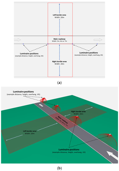
Figure 1.
Overview of the road model setup in ReluxDesktop and used for the calculations. The specific arrangement shown (pole distance, height, overhang, tilt, road width) and the light distribution curves are indicative: (a) Layout of the road geometry and border areas; (b) 3D view of a typical calculation case.
The arrangement of luminaires along the road was selected to simulate the most common situations, but without restricting any potential solution. The main idea behind this decision was to consider all possible lighting designs that could be applied, including the best possible designs, intermediate solutions and very bad lighting designs. These situations can be faced when a light planner/engineer is able to select the suitable combination of light distribution and luminaire arrangement, or, on the contrary, the lighting design is performed without proper knowledge or by other reasons for selection of the equipment and the geometry.
2.2. Luminaire Photometric Data
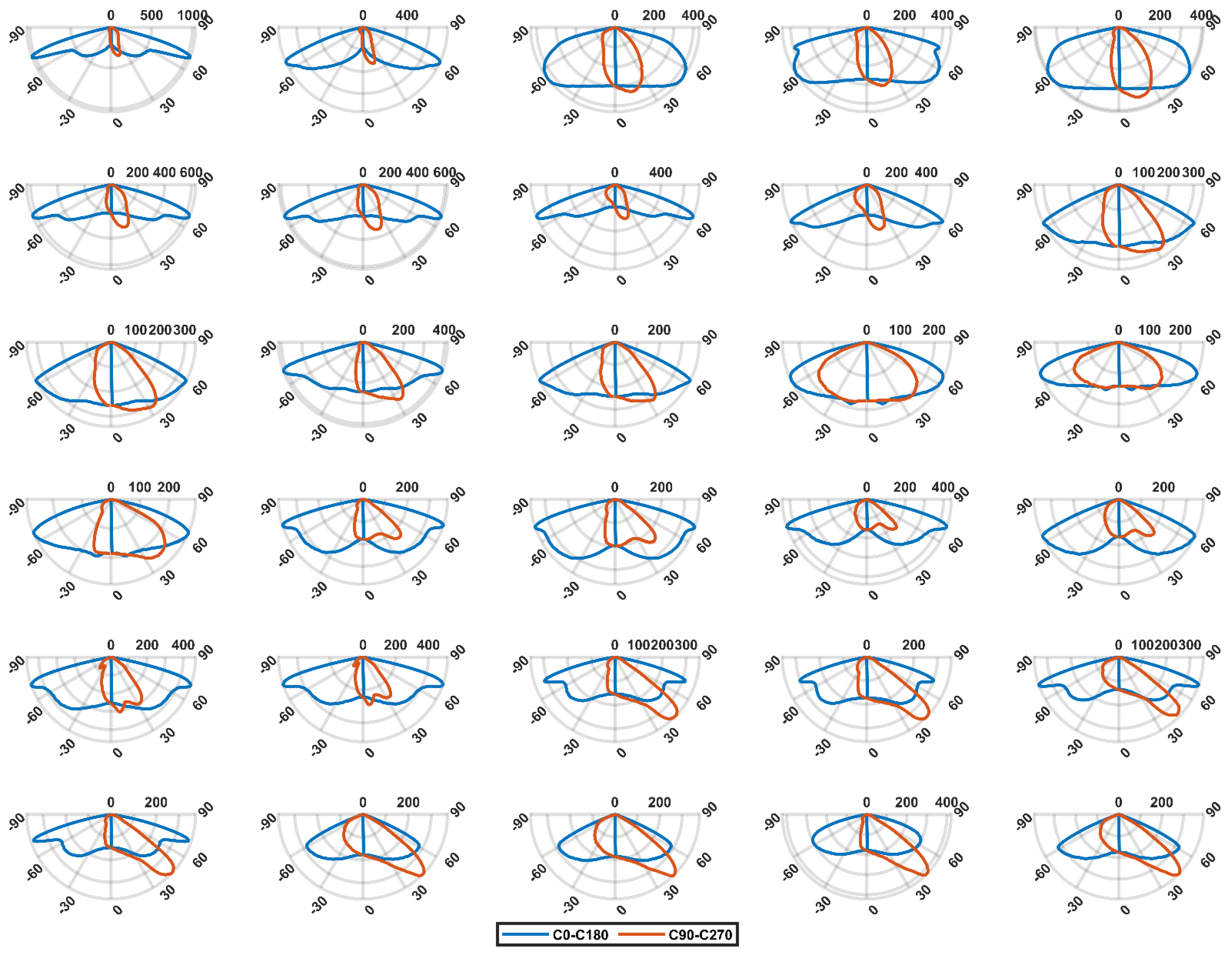
Given the fact that there are hundreds of thousands of different luminaire configurations for street lighting (i.e., power, efficacy, light distribution, etc.), the selection of candidate luminaires in this study focused on alternative lighting distributions. As the distribution of light in the three-dimensional space is independent from the efficacy of the luminaire, all used luminaires were set to have the exact same characteristics, except for the light distribution. For more information on this aspect (normalized luminaire characteristics), see the section “Calculated data and post processing”. An extensive investigation of the potential light distributions for pedestrian and rural road luminaires was made, and a set of 150 different optics (light distribution curves) of LED luminaires were selected and used in the simulations. The light distributions were derived from the corresponding EULUMDAT photometric files of real products from European luminaire manufacturers. All selected luminaires had an upward light ratio (ULR) equal to zero (ULR = 0 or full cut-off), meaning that there was no emission to the upper hemisphere when the luminaire was installed in a horizontal position. Luminaires that may also be used for pedestrian roads having light output ratio (LOR) > 0 were rejected (e.g., pole top traditional shaped lanterns or similar decorative products). The authors decided not to disclose the sources of the photometric files for the following reasons: (a) the study does not focus on the manufacturers themselves but to include as many technical solutions as possible that are available in the market today; (b) many of the selected light distributions included in this study can be offered (identical or almost identical) from more than one manufacturer; and (c) none of the manufacturers influenced the selection of the luminaires. Figure 2 shows the light distribution from 30 representatives (out of 150) of the selected luminaires by means of polar plot of luminous intensity curves. It should be noted that even if some curves in Figure 2 appear almost identical, this is because only the planes C0-C180 or C90-C270 are shown. In the intermediate C-planes, the distribution may be significantly different, and thus it will result in a completely different illumination result on the road and on the surroundings. In addition, many of the selected optics are not suitable for the geometries used in this study (as can be observed by an experienced designer) but were intentionally selected to demonstrate how an improper or random selection of a luminaire configuration can lead to severe issues regarding the illumination of the road and its surroundings.

Figure 2.
Luminous intensity distribution curves of a few representative luminaires (30 out of 150 used in total) in cd/klm. The key C–planes (C0–C180 and C90–C270) are shown for each luminaire.
2.3. Calculated Data and Post Processing
The calculation of the photometric quantities and metrics was performed according to EN 13201-3 [6] using the road calculation core of ReluxDesktop. The calculation parameters and variable geometries were set according to Table 1. The total number of calculated cases was around 1.5 million (i.e., 1,464,750).

Table 1.
Road lighting calculation parameters used in ReluxDesktop.
The calculated quantities and metrics for each applied road geometry and luminaire arrangement depend (apart from the geometry itself) on the power (W), luminous efficacy (lm/W) and LOR of the selected luminaire. Since most of the selected luminaires differ in terms of the above-mentioned characteristics, a normalization process was applied to the calculated data. In addition, a target average illuminance level of 10 lx (class P2) and a luminous efficacy of 120 lm/W were set for a unified comparison of all cases. It should be noted that the same process could be followed for any possible combination of luminous efficacy and targeted average illuminance. The data normalization is summarized as follows:
- A correction factor was calculated for all luminaires to simulate a common efficacy of 120 lm/W.
- A correction factor was calculated for all luminaires to simulate an LOR of 100% (i.e., no internal absorption of luminous flux).
- The required luminaire power for each case was reduced or increased accordingly using the correction factors for the targeted average illuminance of 10 lx. Thus, all cases resulted in exactly 10 lx of average road illuminance, with each one having a “corrected” luminaire power.
- The corresponding calculated metrics (overall uniformity, Uo, and edge illuminance ratio, REI) were kept as calculated, since they are not affected by the achieved levels of illuminance but only by the light distribution from the optics.
At the end of this data processing, all investigated cases have the main road illuminated with an average illuminance of exactly 10 lx. On the other hand, the luminaire power for each case was calculated as the minimum required power of a luminaire that had the same light distribution (lens) and luminous efficacy equal to 120 lm/W. Therefore, all cases presented in Section 3 can be compared equally. Should we want to have the same dataset for, for example, 140 lm/W (instead of 120 lm/W) and/or an average road illuminance of 5 lx (instead of 10 lx), the appropriate correction factors can be directly applied to the raw calculation results.
2.4. Selected Metrics for Analysis
As mentioned, this study performs a sensitivity analysis of the overall uniformity of illuminance against the efficiency of the lighting design, energy-related aspects, and effects on the environment. Therefore, a set of relevant metrics was selected to be calculated and analyzed in correlation with uniformity. Two new metrics related to the impact on the immediate environment are also proposed and defined in this study. Other metrics could also have been selected, but for the purpose of this study, they were omitted as not strictly relevant.
2.4.1. Overall Uniformity
The overall uniformity was calculated as the ratio of minimum to average, directly by ReluxDesktop, and reported for each case. This metric is directly requested by most of the lighting classes (e.g., M and C) but indirectly requested in the P classes. In this case, EN 130201-2 requests that, for example, for the P2 class of 10 lx, the minimum illumination should be at least 2 lx, while the maintained average illuminance should not exceed 15 lx. This results in an overall uniformity of from 0.20 in real design conditions to around 0.13 in the case of increased average illuminance. The same is valid for all P classes (P1–P6). Thus, the boundaries for the required overall uniformity in the P class are 0.13 to 0.20, whereas in the M and C classes, it varies from 0.35 to 0.40.
In many cases, in real installations, lighting designers tend to follow the suggestion for uniformity of 0.4 or above independently of class. The effects of such a decision will be presented in the results and will be discussed later in this paper.
2.4.2. Minimum Luminaire Power
This simple metric calculates the minimum luminaire power that is needed to achieve an average illuminance on a road surface equal to 10 lx under the given efficiency parameters (i.e., 120 lm/W and LOR = 1.0). Therefore, the same luminaire using the same optic may need different electric power to achieve 10 lx in a different arrangement. This is the above-mentioned normalization process for all investigated cases. The per-case minimum luminaire power was calculated according to the process described in Section 2.3. Therefore, the luminaire power shown in various figures corresponds to the minimum required power.
2.4.3. Energy Performance and Power Density Indicator (PDI)
The energy performance is assessed using the specific power density indicator (PDI, in W·lx−1·m−2 [32], abbreviated as DP). The use of PDI for evaluating the energy efficiency of road lighting installations has been established internationally in the European Standard for Road Lighting. This metric reveals the efficiency of the lighting design in terms of the suitability of the selected light distribution, together with the luminous efficacy of the luminaire under a given road geometry. Lower PDI means that less power is needed to illuminate the area under consideration and, thus, more efficiently designed road lighting. In addition, luminaires with the same efficacy but with different optics may have different PDI, and this reveals that the configuration with lower PDI directs more light toward the area under consideration rather than to the outside of the road.
PDI is calculated with the following formula:
where
- P: the system power of the lighting installation used to light the relevant areas (in W)
- : the maintained average horizontal illuminance of the sub-area “i” (in lx)
- : the size of the sub-area “i” lit by the lighting installation (in m2)
- n: the number of subareas to be lit.
2.4.4. Edge Illuminance Ratio (REI)
The edge illuminance ratio (REI) is defined in EN 13201-2 as “average horizontal illuminance on a strip just outside the edge of a carriageway in proportion to the average horizontal illuminance on a strip inside the edge, where the strips have the width of one driving lane of the carriageway” and is used to ensure a certain amount of illumination on nearby roadside areas to improve visibility for side areas and to increase traffic safety. For example, if there are P-class roads without lighting alongside the motorized road, it is important to be able to view users. Although this metric is only used in M classes, it was selected for calculation in this study to reveal the spread of light beyond the borders of the road and was used for comparisons with the new metrics for spill light. The calculation was made according to EN 13201-3 [6].
2.4.5. Extended Edge Illuminance Ratio (Extended REI)
To investigate the extension of the spill light in both directions of the road, we introduce a new metric named the extended edge illuminance ratio (extended REI). Extended REI was calculated as the average horizontal illuminance up to 20 m from the road edge (on both sides, as shown in Figure 1) to the average horizontal illuminance on the road surface. Estimations of the amount of illuminance reaching the ground layer on borders along the road edge were used in a previous study and showed that it is a useful approach for assessing the environmental impacts of lighting installations [33]. It estimates how light from the installations propagates into the adjacent road environment and the nearby natural environment. The amount of spill light on adjacent areas enables assessment of the ecological impact of road lighting on ground-living organisms, such as mammals, amphibians, insects, and plants. However, under natural field conditions, the roadside structure is usually not flat, as in the simulations, but consists of subareas situated at various distances and at various inclinations in relation to the roadway, such as a shoulder, side slope, ditch, backslope, and natural ecosystems [34]. The extended REI reveals how the selection of optimum-considered optics may affect the illumination of the surroundings beyond the road edge and how this is linked to the desired overall uniformity of the road surface. The extended REI can also be estimated using field measurements, especially novel methods developed using aerial measurement devices such as the drone-goniophotometer [35].
2.4.6. Spill Flux Ratio (RSF)
To assess the overall efficiency of the lighting design per case in terms of spill luminous flux and, therefore, the potential risk for light pollution on the surrounding ground along the roadway, we introduce a new metric named spill flux ratio (RSF). Spill flux ratio is the proportion of the luminous flux of a lighting installation emitted in the total border area when the luminaire(s) is (are) mounted in its (their) installed position. The spill of luminous flux is calculated in this study as the percentage of spill light (spill luminous flux) that propagates outside the road surface to the total luminous flux produced by the luminaires. The total border area (m2) is calculated by the pole distance times 20 m on each side of the road (see Figure 1). In this study, the RSF was calculated using total luminous flux, which is calculated by the normalized power of the luminaire under an efficacy of 120 lm/W (see Section 2.3). However, this percentage does not change under different efficacies since it is only related to the light distribution of the optics and the road/installation geometry.
2.5. Big Data Analysis and Illustrations
The analysis of the big data set of the photometric calculations was conducted using the assistance of specific plots. Since the amount of data was huge, a case-by-case investigation was practically impossible. For these reasons, we present groups of three types of figures. Each group investigated the correlation between the overall uniformity and the other selected metrics. The three figure types are explained below.
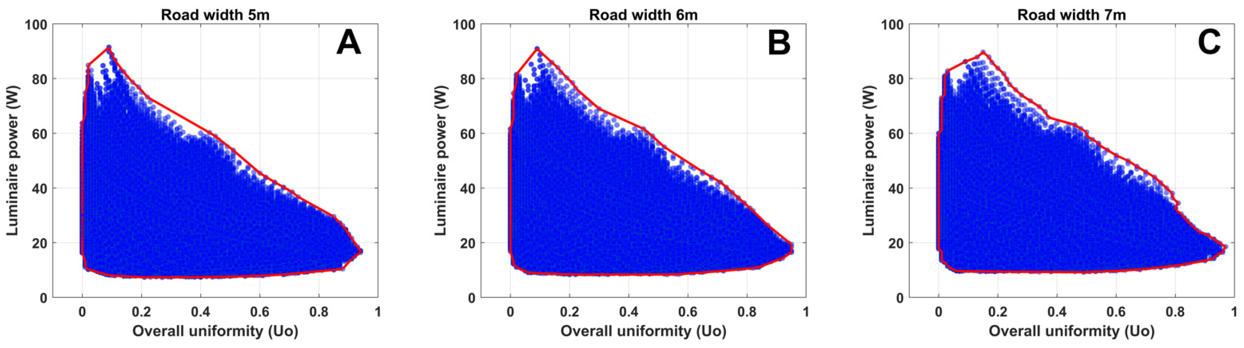
- Figure type 1—All calculated cases
These figures illustrate the total number of calculated cases classified by road width. The results of each case (e.g., the luminaire power vs. uniformity) are presented with one blue dot. Since the total number of cases per road width is around half a million, they appear as a continuous blue area. A red line outlines the boundaries of the plotted data, representing the technical boundaries (or limitations) related to the selected luminaire types. In this blue area, all kinds of cases (good, intermediate, bad) are included. Since the selected light distributions are considered representative for most of the luminaire manufacturers, the red outlined boundary is in line with what is expected in reality.
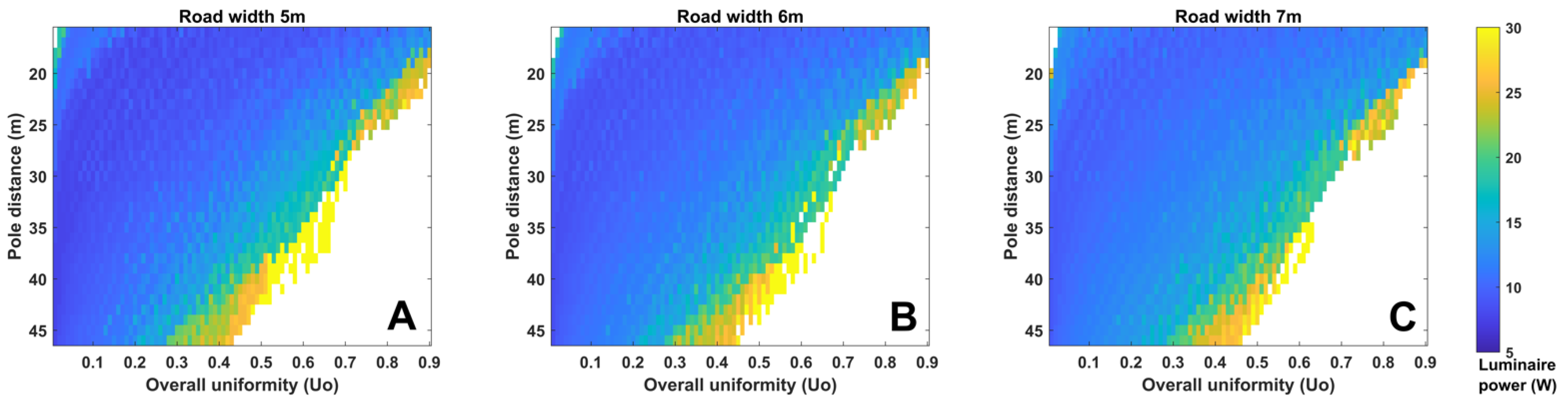
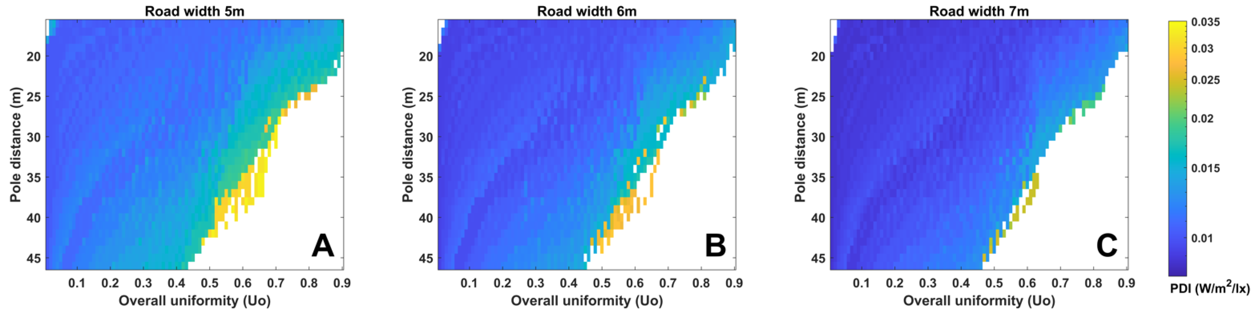
- Figure type 2—Lower quantities per uniformity and road width
These figures illustrate a subset of Type 1 figures. In particular, they present the lowest calculated values of the selected metric (e.g., the luminaire power) for every possible combination of uniformity and pole distance, independent of the rest of the geometry characteristics (i.e., height, overhang, etc.). There is one figure per road width. The value of the selected metric is presented on a color scale. White space means that there is no technical solution for the combinations of uniformity and pole distance. Therefore, these figures act as a lookup table (or a map) of the technically expected lower value of the presented metric per uniformity and pole distance.
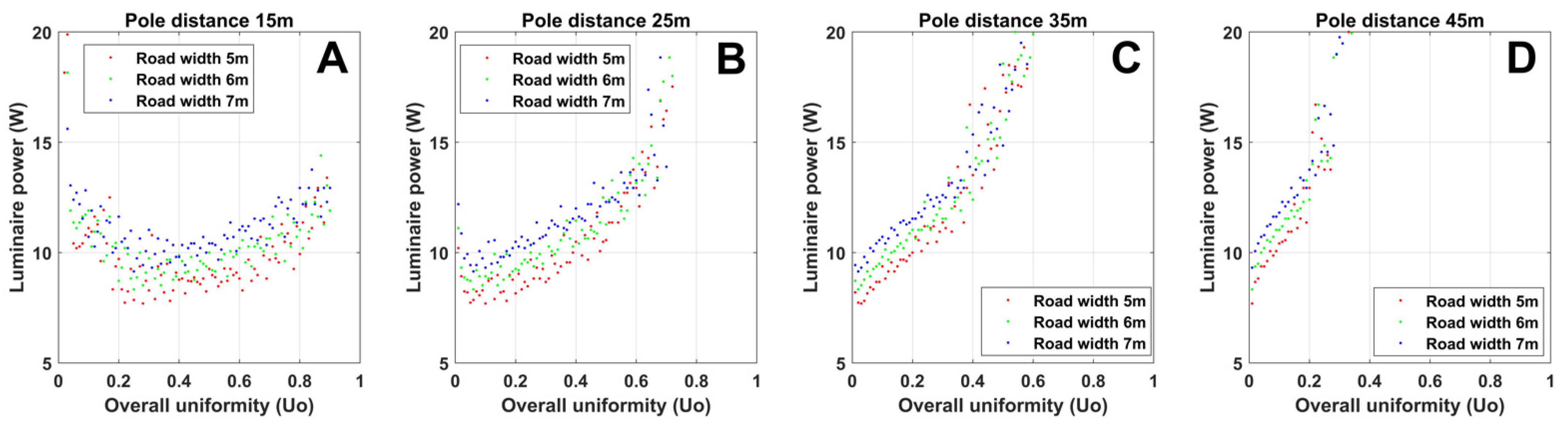
- Figure type 3—Lower quantities per uniformity, road width, and selected pole distances
The third type of figure presents an even smaller subset of the overall dataset. In this case, the plotted data correspond to the minimum value of the selected metric against all potential uniformities for a few representative pole distances (15 m, 25 m, 25 m, and 45 m) and for the three distinctive road widths (5 m, 6 m, and 7 m). Specific pole distances were selected because they represent common selected values. The plots are horizontal sections of the corresponding figures of type 2 at distances of 15 m, 25 m, 25 m, and 45 m, respectively. Using this type of figure, one can clearly assess the influence of the pole distance on the achieved uniformity and how this affects the minimum value of the selected metric.
3. Results
The analysis results are presented in five groups consisting of the above-presented three types of figures. Each group refers to a specific metric, namely, the installed power of the luminaire, the DP, the REI, the extended REI and the RSF.
3.1. Overall Uniformity vs. Luminaire Power
The first set of figures (Figure 3, Figure 4 and Figure 5) presents the calculation results of the uniformity on the road versus the installed power of the luminaire that is needed to achieve 10 lx. Luminaire power is strictly related to the energy consumption of the installation. Figure 3 includes all calculated cases (around half a million for each road width) surrounded by a red boundary line, indicating all technically possible solutions. The bottom side of each sub-figure in Figure 3A–C reveals the lowest installed power of the luminaire that is technically possible (given the selected optics) to achieve the corresponding uniformity. For the investigated road widths and for the target illuminance of 10 lx, any uniformity up to 0.8 for 5 m width, 0.7 for 6 m width, and 0.6 for 7 m width can be achieved using around 8–10 W of installed luminaire power. Further increase of the required uniformity will result in a slight increase in the installed power, which is demonstrated by the increased slope of the bottom red line.
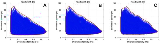
Figure 3.
Overall uniformity of illuminance vs. required luminaire power for Em = 10 lx. The graphs include all potential pole arrangements, as shown in Table 1: (A) results for road width of 5 m; (B) results for road width of 6 m; (C) results for road width of 7 m.
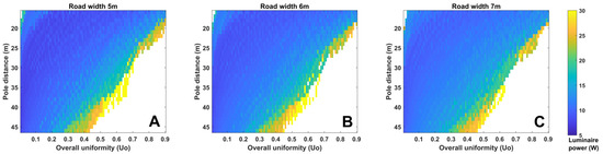
Figure 4.
Overall uniformity of illuminance vs. pole distance vs. minimum luminaire power for Em = 10 lx. Dark blue indicates low power, whereas yellowish refers to higher power levels. The white space equals a lack of technical solutions: (A) results for road width of 5 m; (B) results for road width of 6 m; (C) results for road width of 7 m.
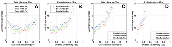
Figure 5.
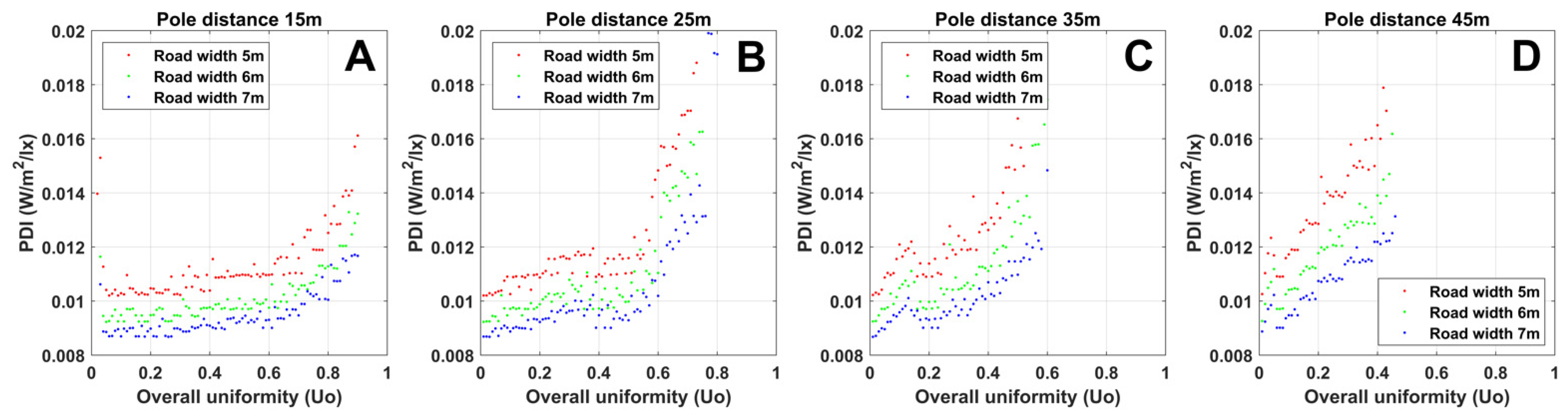
Overall uniformity of illuminance vs. minimum luminaire power for Em = 10 lx for key pole distances: (A) results for pole distance of 15 m; (B) results for pole distance of 25 m; (C) results for pole distance of 35 m; (D) results for pole distance of 45 m.
Figure 4 presents the minimum required luminaire power to achieve a desired uniformity under a given pole distance (and vice versa) for the target average road illuminance of 10 lx. If the main assessment criterion is energy consumption, one should consider utilizing solutions around the darkest blue regions. However, this may result in lower uniformity on the road surface. For all road widths, it is clearly shown that it is easier to achieve a high uniformity (>0.2) with shorter pole distances, but this also depends on the pole height for the installation (data for pole heights are not shown). A uniformity of 0.2 can be achieved with most pole distances and road widths with a luminaire power < 15 W.
Figure 5 plots the sections of Figure 4 for all road widths for the key pole distances of 15 m, 25 m, 35 m, and 45 m. Each subfigure refers to a specific pole distance, while the results for all road widths are plotted together. All have a vertical scale of up to 20 W for an improved comparison. Figure 5 shows that, for all road widths, the corresponding plots have similar trends, but the average slope of the plotted curves shows a significant difference when increasing the pole distance. For example, in Figure 5B, for pole distances of 25 m, a uniformity of 0.2 can be achieved at around 8 W to 10 W (depending on the road width). With the same uniformity for a pole distance of 35 m (Figure 5C), the minimum required power increases from 10 W to 12 W (again, depending on the road width). On the other hand, if one wants to increase the uniformity from 0.2 to 0.4, keeping the 35 m spacing (Figure 5C), the expected increase in luminaire power is at least around 30%. Similar results can be drawn for other levels of uniformity.
3.2. Overall Uniformity vs. PDI
The second set of figures (Figure 6, Figure 7 and Figure 8) presents the calculation results of the uniformity on the road versus the PDI when the target road illuminance is 10 lx. The PDI versus uniformity reveals the possible compromised energy efficiency of the installation in case one needs to achieve better uniformity.
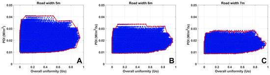
Figure 6.
Overall uniformity of illuminance vs. PDI; simulation results for all cases (around half a million for each road width) surrounded by the red boundary line of the technically possible solutions. The graphs include all potential pole arrangements, as shown in Table 1: (A) results for road width of 5 m; (B) results for road width of 6 m; (C) results for road width of 7 m.
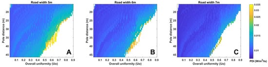
Figure 7.
Overall uniformity of illuminance vs. pole distance vs. minimum PDI The PDI was presented on a color scale. The dark blue color indicates a low PDI, whereas yellowish colors refer to higher PDI levels. The white space equals a lack of technical solutions: (A) results for road width of 5 m; (B) results for road width of 6 m; (C) results for road width of 7 m.
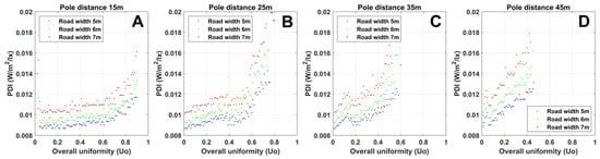
Figure 8.
Overall uniformity of illuminance vs. minimum PDI for key pole distances: (A) results for pole distance of 15 m; (B) results for pole distance of 25 m; (C) results for pole distance of 35 m; (D) results for pole distance of 45 m.
For the investigated road widths and for the target illuminance of 10 lx, any uniformity up to 0.6 can be achieved under a PDI of around 0.008 W/m2/lx to 0.010 W/m2/lx, see Figure 6A–C. Further increase of the required uniformity will result in a slight increase in PDI (the sloped section of the bottom red line).
Figure 7 presents the minimum PDI to achieve a desired uniformity under a given pole distance (and vice versa) for the target average road illuminance of 10 lx. Therefore, in cases where the assessment criterion is the energy efficacy of the road installation (e.g., according to EN 13201-5), one should consider utilizing solutions around the darkest blue regions. However, this may result in lower uniformity on the road surface. In all Figure 7A–C, there is a clear indication of a region of optimum solutions (related to PDI) for each uniformity indicated by the dark blue color. This is shown similar to a dark blue “river” starting close to the Uo = 0.1 and 45 m pole distance combination toward Uo = 0.3 and 25 m pole distance, and so on. This dark blue “river” is slightly different for each road width, but it clearly shows the regions with the lowest PDIs.
Figure 8 shows sections of Figure 7 for all road widths but for key pole distances of 15 m, 25 m, 35 m, and 45 m. Each subfigure refers to a specific pole distance, while the results for all road widths are plotted together. All plots had a vertical scale of up to 0.02 W/m2/lx for a better comparison. Figure 8 shows that, for all road widths, the corresponding plots have similar trends, but the average slope of the plotted curves shows a significant difference by increasing the pole distance. For example, in Figure 8A, for pole distances of 15 m, a uniformity of 0.2 results in a PDI between 0.0085 and 0.011, depending on the road width. The same uniformity for a pole distance of 45 m (see Figure 5D) resulted in an increased PDI of between 0.010 and 0.013 (again, depending on the road width). Since the PDI is strictly related to the geometry of the installation and the optics used, there are cases in which specific solutions for a given uniformity result in a lower PDI compared to the uniformities in proximity (i.e., local minima at the uniformity of 0.4 in Figure 8B and uniformity of 0.2 in Figure 8C). Similar results can be drawn for other uniformities. The overall remark is that higher uniformity under larger pole distances results in increased PDI values and is thus a less efficient lighting design.
3.3. Overall Uniformity vs. REI
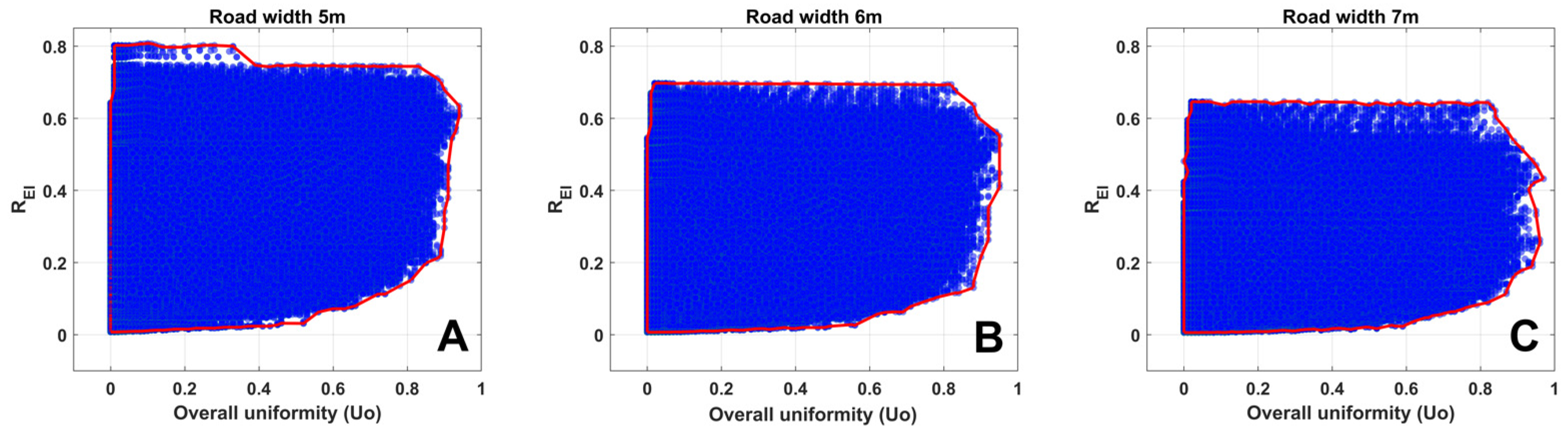
Figure 9 illustrates all calculated cases (around half a million for each road width) surrounded by the red boundary line of the technically possible solutions, and the bottom side of each sub-figure A, B, and C of Figure 9 reveals the lowest REI that is technically possible (given the selected optics) to achieve the corresponding uniformity. Figure 10 shows that for the investigated road widths, the increase in the required uniformity will result in a slight increase in the REI (sloped section of the bottom red line). The narrower road (5 m) has a steeper slope due to the technical difficulty of keeping the light inside the road boundaries. This is also exemplified by many cases that have a higher REI (up to 0.8) in the upper part of Figure 9A.

Figure 9.
Overall uniformity of illuminance vs. REI, simulation results for all cases. The graphs include all potential pole arrangements, as shown in Table 1: (A) results for road width of 5 m; (B) results for road width of 6 m; (C) results for road width of 7 m.
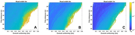
Figure 10.
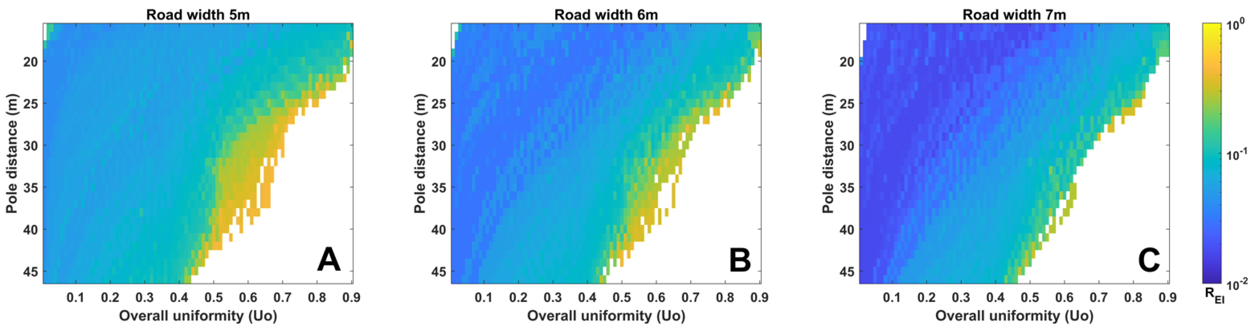
Overall uniformity of illuminance vs. pole distance vs. minimum REI. Dark blue indicates a low REI whereas yellowish refers to higher REI levels. The white space equals a lack of technical solutions: (A) results for road width of 5 m; (B) results for road width of 6 m; (C) results for road width of 7 m.
Figure 10 presents the minimum REI as a result of the corresponding uniformity under a given pole distance (and vice versa). To achieve the solution with the lowest REI, for example, when a minimal impact on the environment is wanted, solutions in the darkest blue regions are considered the most optimal (Figure 10A–C). The dark blue regions of the minimum REI are most often associated with lower uniformities and shorter pole distances. In opposite situations, the REI increases.
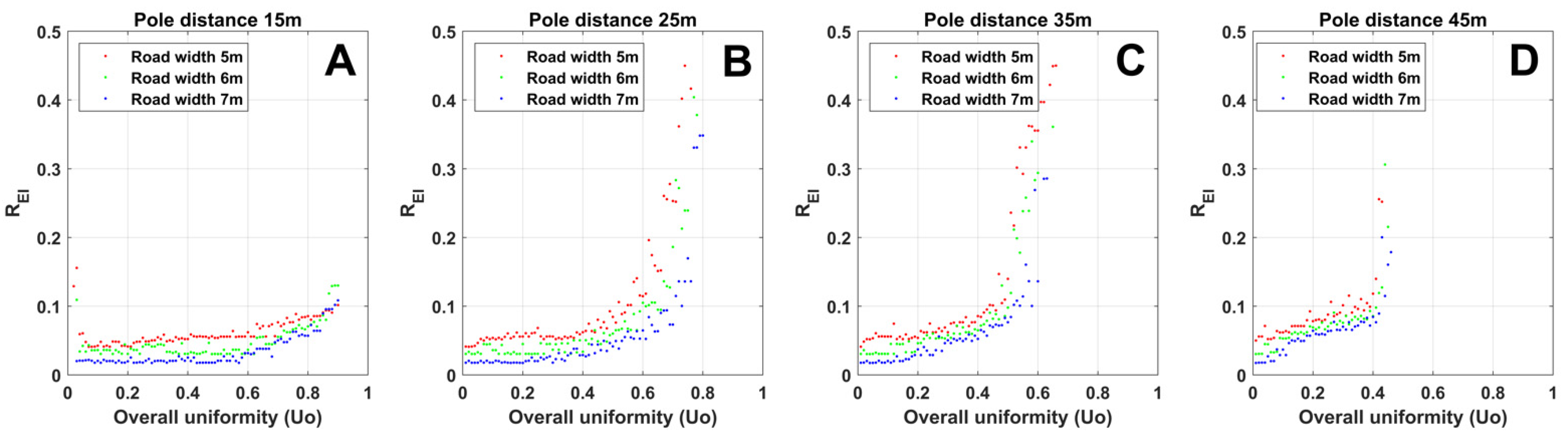
Figure 11 shows that for all road widths, the corresponding plots have a similar shape, but the average slope of the plotted curves shows a significant difference by increasing the pole distance. For all pole distances except for 15 m, the REI gently increases as the uniformity increases up to a certain point where the increase is very steep (i.e., around 0.6–0.7 in a 25 m pole distance, around 0.5 in a 35 m pole distance, and above around 0.4 in a 45 m pole distance). Therefore, higher uniformity under larger pole distances results in stepwise higher REI values and thus more light will be directed to the immediate surroundings of the road, whereas after a certain tipping point of overall uniformity, the REI increases dramatically, almost vertically.
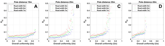
Figure 11.
Overall uniformity of illuminance vs. minimum REI for key pole distances. Only REI ≤ 0.5 is included: (A) results for pole distance of 15 m; (B) results for pole distance of 25 m; (C) results for pole distance of 35 m; (D) results for pole distance of 45 m.
3.4. Overall Uniformity vs. Extended REI
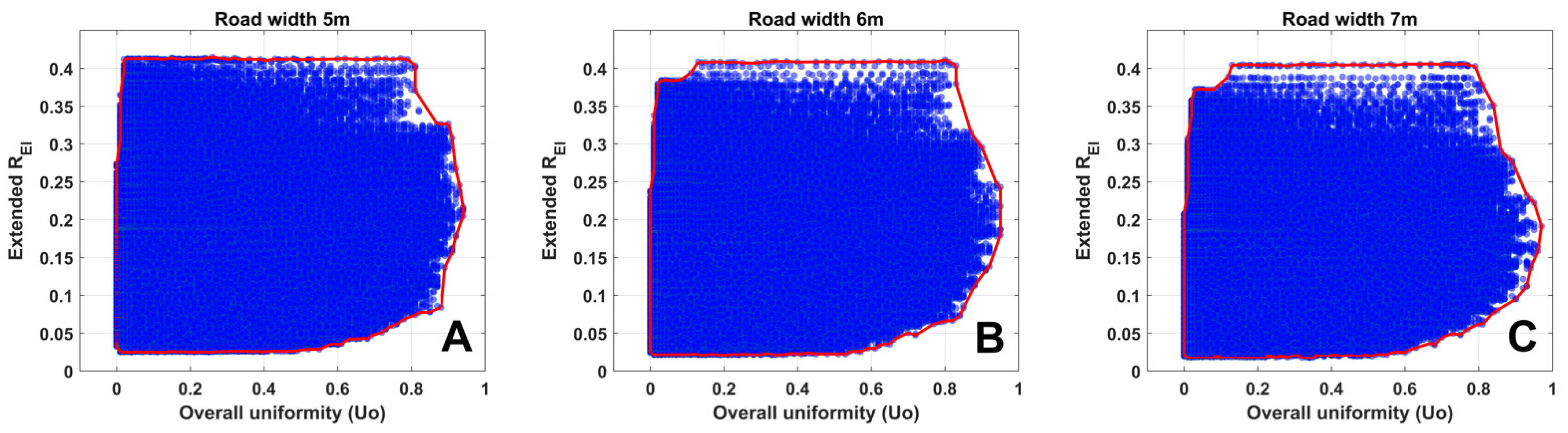
The set of Figure 12, Figure 13 and Figure 14 presents the calculation results of the overall illuminance on the road versus the extended REI as this was defined in Section 2.4. This comparison assesses how a selected lighting design, with respect to good uniformity, may affect the illumination of the surroundings up to 20 m beyond both sides of the road.
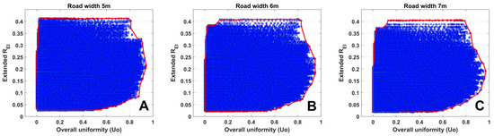
Figure 12.
Uniformity vs. Extended REI (up to 20 m left and right). Simulation results for all cases. The graphs include all potential pole arrangements, as shown in Table 1: (A) results for road width of 5 m; (B) results for road width of 6 m; (C) results for road width of 7 m.
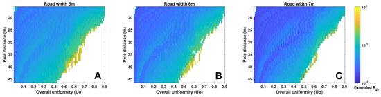
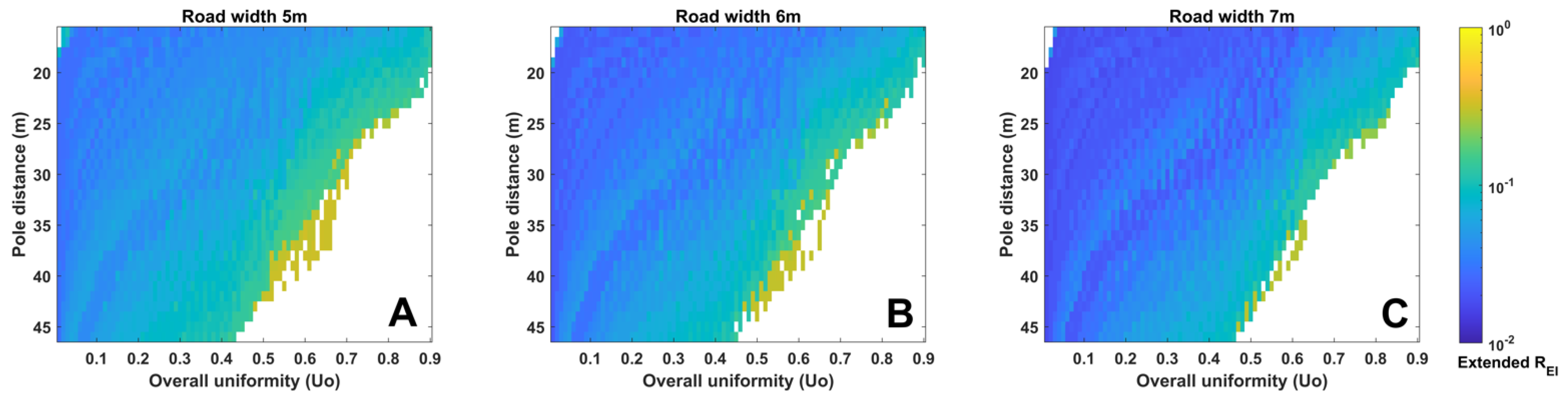
Figure 13.
Overall uniformity of illuminance vs. pole distance vs. minimum extended REI. The dark blue color illustrates a low extended REI whereas yellowish colors refer to higher extended REI levels. The white space equals a lack of technical solutions: (A) results for road width of 5 m; (B) results for road width of 6 m; (C) results for road width of 7 m.
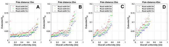
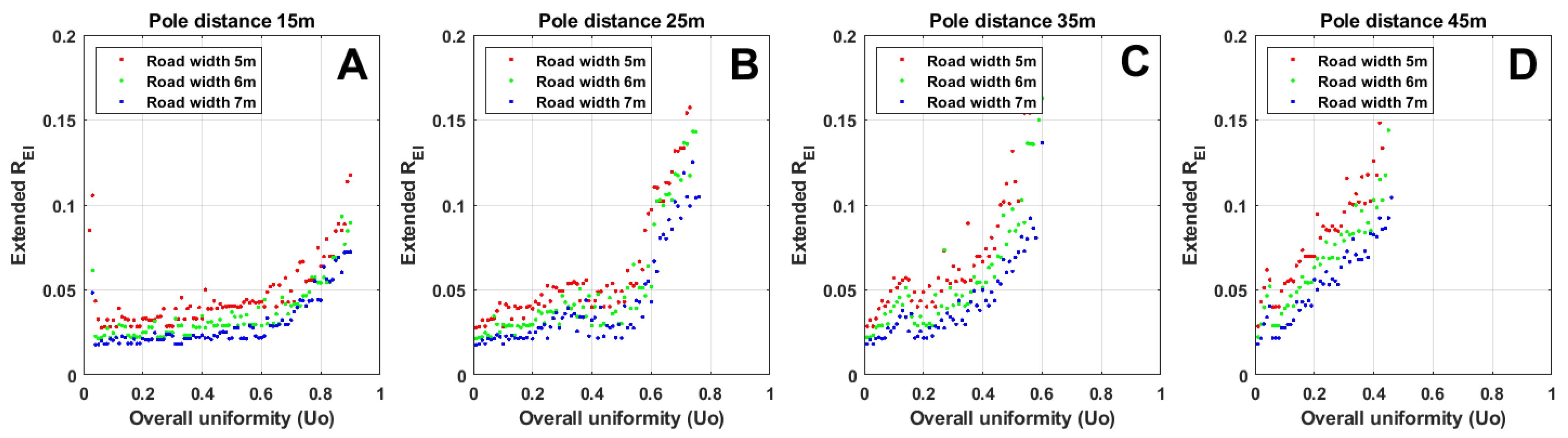
Figure 14.
Overall uniformity of illuminance vs. minimum extended REI for key pole distances. Only REI ≤ 0.2 is included: (A) results for pole distance of 15 m; (B) results for pole distance of 25 m; (C) results for pole distance of 35 m; (D) results for pole distance of 45 m.
Figure 12 illustrates all calculated cases (around half a million for each road width) surrounded by the red boundary line of the technically possible solutions. The bottom side of each sub-figure A, B, and C of Figure 12 reveals the lowest values of the extended REI that is technically possible (given the selected optics) to achieve the corresponding overall uniformity. Figure 12 shows that for the investigated road widths, the increase in the required uniformity will result in a slight increase in the extended REI (sloped section of the bottom red line). There are indications of a steeper slope on the narrower road (5 m) due to the technical difficulty of keeping the light inside the road boundaries. However, Figure 12A–C have very similar bounding areas indicating a small influence of road width in the calculation of the extended REI.
Figure 13 presents the minimum extended REI as a result of the corresponding uniformity under a given pole distance (and vice versa). Cases with the lowest extended REI can be found in the streaks with dark blue areas in Figure 13A–C. The lowest possible extended REI is associated with lower uniformity and shorter pole distances. In the opposite situations, the REI increases.
Figure 14 shows the sections of Figure 13 for all road widths but for key pole distances of 15 m, 25 m, 35 m, and 45 m. Each subfigure refers to a specific pole distance, while the results for all road widths are plotted together. All plots have a vertical scale in extended REI of up to 0.2 for a better comparison. Figure 14 shows that for all road widths, the corresponding plots have a similar shape, but the average slope of the curves shows a significant difference by increasing the pole distance. For all pole distances except 15 m, the extended REI increases slowly as uniformity increases. Therefore, higher uniformity and larger pole distance increases extended REI and thus more light is directed to the surroundings of the road (up to 20 m away).
3.5. Overall Uniformity vs. Spill Flux Ratio
For the investigated road widths for any required uniformity, there will be a constant minimum value of RSF, which will increase with the increase of uniformity, as can be seen in the sloped section of the bottom red line in Figure 15A–C.
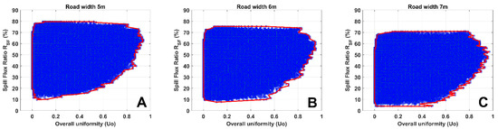
Figure 15.
Overall uniformity of illuminance vs. spill flux ratio, simulation results for cases. The graphs include all potential pole arrangements, as shown in Table 1. The red boundary line indicates the technically possible solutions. The bottom side of each sub-figure A, B, and C of Figure 15 reveals the lowest percentage of spill luminous flux that is technically possible (given the selected optics) to achieve the corresponding uniformity: (A) results for road width of 5 m; (B) results for road width of 6 m; (C) results for road width of 7 m.
There is a visible rock-bottom value of a specific minimum percentage of spill flux clearly demonstrated for each road width, namely, ~15% for 5 m (Figure 15A), ~10% for 6 m (Figure 15B), and ~7.5% for 7 m road width (Figure 15C). Therefore, it is not possible for any scenario to achieve a lower spill flux ratio, irrespective of the lighting design. On the other hand, if, for example, the overall uniformity of a 5-m-wide road is targeted to 0.7, it will result in a minimum of 30% of the luminous flux outside of the road area. The uniformity level above which the RSF increases in a sharper way (the threshold uniformity) is around 0.2 for 5 m width and between 0.5 and 0.6 for 6 m and 7 m width roads.
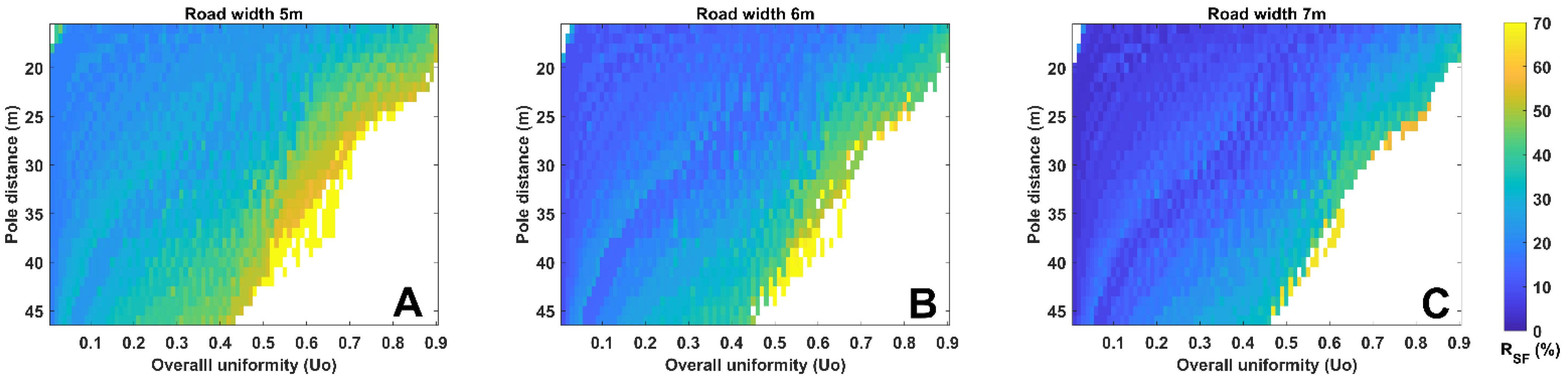
In all Figure 16A–C, there is a clear indication of a set of optimum solutions (related to spill luminous flux) for each uniformity value. This is demonstrated as dark blue patterns (rivers) starting close to 0.08 (Uo) and 45 m combination toward 0.2 (Uo) and 35 m and so on. This dark blue river is slightly different for each road width, but it clearly shows the regions with the lowest percentage of spill luminous flux. The dark blue regions are most frequent when uniformity is lower and pole distance is shorter. In opposite situations, the percentage of spill luminous flux increases.
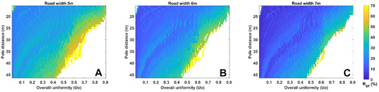
Figure 16.
Overall uniformity of illuminance vs. pole distance vs. minimum spill flux ratio. Dark blue indicates a low percentage of spill luminous flux, whereas yellowish refers to a higher percentage of spill luminous flux levels. The white space equals a lack of technical solutions: (A) results for road width of 5 m; (B) results for road width of 6 m; (C) results for road width of 7 m.
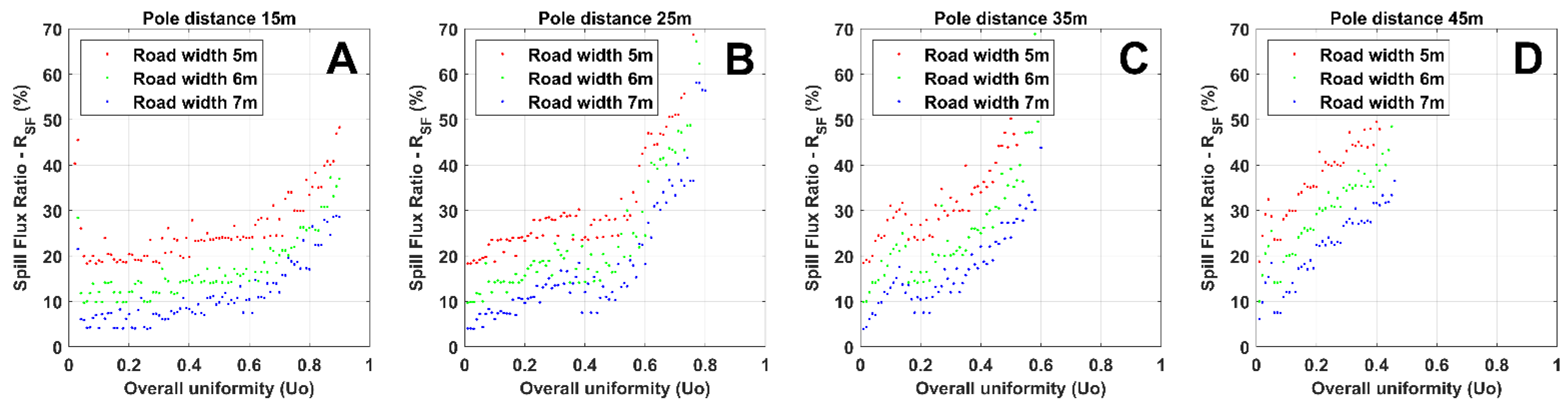
Figure 17 shows that for all road widths, the corresponding plots have a similar shape, but the average slope of the curves shows a significant difference by increasing the pole distance. For all pole distances, the percentage of spill luminous flux increased with uniformity. Therefore, a higher uniformity under a larger pole distance results in a higher percentage of spill luminous flux and more light falls outside of the road area. In addition, the percentage of spill luminous flux shows a constant, almost flat value in 15 m pole distance for up to an overall uniformity of 0.6.
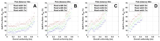
Figure 17.
Overall uniformity of illuminance vs. minimum spill flux ratio for key pole distances. All plots have a vertical scale in percentage of spill luminous flux of up to 70% for a better comparison: (A) results for pole distance of 15 m; (B) results for pole distance of 25 m; (C) results for pole distance of 35 m; (D) results for pole distance of 45 m.
4. Discussion
We have shown that the optimization of the lighting design by utilizing the proper light distributions (i.e., lenses/reflectors) leads to a reduction of the installed power (and consequently the consumed energy) and of the impact on the surrounding areas in terms of spill light. The calculations included a large set of representative light distributions (150 of them) under various typical geometries for pedestrian roads. Therefore, it can be stated that the results represent most real-life situations.
In this study, we found that the ambition for increased overall illuminance uniformity on the road surface can significantly impact energy consumption and the surrounding environment through spill light, especially when the lighting planning process prioritizes uniformity. Among hundreds of thousands of different solutions, the most optimal solutions can keep adverse effects at low levels. However, aiming for uniformities above the minimum requirements may lead to severe trade-offs in energy use and increases in spill light. Lighting professionals who are responsible for road lighting design are, in many or most cases, working with a limited amount of photometric data, which leads to a reduced number of potential solutions. These solutions can also be found in our big dataset of simulations, which is presented in the figures, but it is unlikely that they are the best or the optimum solutions.
Pedestrian reassurance in residential roads was shown to increase with higher uniformity in a study by Fotios et al. that was performed in field conditions on roads with a horizontal illuminance uniformity between 0.12–0.56 and pole distances between 23.2–39.2 m [15]. Seven of the ten included roads in that study had an illuminance uniformity ≥ 0.24, which is well above the uniformity recommended by the European Road Lighting Standard for pedestrian P-class lighting roads of 0.13–0.20 [8]. The study by Fotios et al. [18] shows that an illuminance uniformity of around 0.3–0.56 can be more beneficial for pedestrians since the safety rating difference between day-dark is closer to zero in comparison with lower uniformities (0.12–0.26). This indicates that for pedestrians, a recommended uniformity of 0.13–0.20 may be too low if high reassurance is wanted. However, the study by Fotios et al. included only 10 test locations/roads, of which one location was a park pathway and another was an underpass. It is currently unknown whether the results are generally valid for, for example, other road types, lighting designs, environments, and countries, since this has not yet been investigated. However, it is possible for two roads with the same level of illuminance uniformity (0.16 and 0.17) to differ in perceived uniformity [24], because other elements in the road environment can have a high influence on the overall visual perception for an observer. For pedestrian road lighting, the perceived lighting uniformity and visual impressions of the road environment relate to the full spatial context and attributes of the entire visual scene and are dependent upon the location of the observer [11]. In terms of pedestrian reassurance, road surface uniformity may be of smaller importance than other elements and structures along the road [11].
Aiming for higher uniformity may be beneficial for reassurance for pedestrians, but it is uncertain whether this holds true when it comes to the visual perceptions of the entire road environment. Nonetheless, it will result in a high risk of increasing energy consumption as well as light pollution via increased spill light in the roadside surroundings, as we have shown in this study. The value of uniformity, above which the trade-offs in energy and spill light increase significantly, differs according to road width, but it can be clearly identified in the figures (see the Results section). Even if the requested overall uniformity in pedestrian roads is between 0.13 and 0.2, under some circumstances, it is relevant to achieve uniformities more similar to the ones of a motorized traffic road (e.g., above 0.4) or even as high as 0.5–0.6, for example, if there is mixed traffic (both motorized and pedestrians). For a road that is 7 m wide and has a 35 m pole distance, the increase in overall uniformity from 0.2 to 0.4 may lead to at least a 30% increase in energy consumption and at least a 100% increase in spill light (see Figure 5C and Figure 16C). Similar conclusions can be drawn for other situations, but for shorter pole distances, an increased uniformity did not result in a similar high increase in spill light.
The simulation results were presented with the overall uniformity of horizontal illuminance on the road surface as a key metric. This metric was selected as the most convenient and understandable ratio in lighting engineering. On the other hand, one can easily calculate the minimum value of illuminance via uniformity, using the definition of the metric. For example, in the presented results, since the average illuminance is in all cases 10 lx, a uniformity of 0.2 means a minimum illuminance of 2 lux, and so on. This relation is equal for any given average road illuminance (e.g., for other P classes). Therefore, to achieve a specific minimum illuminance on various P-class roads, one must achieve the corresponding uniformity, which will reflect a specific minimum waste of energy and luminous flux compared to a lower targeted minimum illuminance (or uniformity).
The two new metrics, extended REI and spill flux ratio (RSF) are proposed in this study to be used in combination with the existing metrics of the energy performance criteria but with respect to the environmental impact of the lighting design. Both metrics were designed to evaluate lighting installation performance. The extended REI reveals the portion of light that falls outside the needed area into the immediate environment of the road. The RSF on the other hand, calculated the percentage of the luminous output of the luminaires that is directed outside the road and can also be quantified as a source of light pollution, intrusive light and, in general, a source of obtrusive light. The same metric can also be used as a spill energy metric, since the wasted luminous flux is directly proportional to the energy that is consumed to produce it. The simulation results also show that the spill luminous flux is concentrated inside the border areas of 20 m (left and right sides of the road) in more than 95% of the simulated cases (not reported). In the other 5% of the cases, only around 2.5% of the spill flux was directed outside the 20 m borders and potentially upwards (mainly cases with positive luminaire tilt). Therefore, it is suggested that the 20 m border limit is sufficient for the calculation of spill flux and can be easily introduced in road calculation software.
Extended REI and spill flux ratio can be used to assess the environmental impact in terms of the amount of illuminance spilling on the roadside area adjacent to the road in comparison with the amount on the road surface. Such roadside areas are typically not classified as “natural” habitats or ecosystems, since the road verge, ditch, and backslope are manmade from the road construction. Nevertheless, parts of the roadside area, for example, the backslope and the surrounding landscape, are inhabited by natural species due to the successive intrusion of species from the surrounding areas into the roadside. In future studies, it would be useful to divide the roadside area into segments and report the mean, maximum, and minimum illuminance levels for each segment, since this information is essential for assessing the ecological impact on specific species. Depending on the characteristics of the landscape and the road environment, it may also be necessary to adapt the size of the border area when assessing the environmental impact of the light at night.
This study did not include upward emitted light or reflected light, which has often been the focus of studies in the past when investigating light pollution, especially from the perspective of astronomical light pollution. However, it would be beneficial to include parameters of the upward emitted light, reflectivity of the ground, and other structures contributing to skyglow and color temperature of light sources in a future study. For example, both the upward light ratio, ULR, and the upward flux ratio, UFR, can be used to estimate the astronomical impact (i.e., sky glow) in a future study based on the same dataset of simulations. Both ULR and UFR are recommended for use in the CIE report “Guide on the limitation of the effects of obtrusive light from outdoor lighting installations” [36].
Author Contributions
Conceptualization, A.K.J. and C.A.B.; methodology, A.K.J. and C.A.B.; software, C.A.B.; validation, C.A.B.; formal analysis, C.A.B.; data curation, C.A.B.; writing—original draft preparation, review and editing, A.K.J. and C.A.B.; visualization, C.A.B. All authors have read and agreed to the published version of the manuscript.
Funding
This research was funded by Bertil and Britt Svenssons stiftelse för belysningsteknik grant number “Ansökningsnummer 2020 vår-22” and “Ansökan 2021 vår-10” (to A.K.J.).
Acknowledgments
The authors want to acknowledge Relux Informatik A.G. for their support regarding the lighting calculation method and the tools provided. This work is the first part of a collaborative project on the environmental impact of road lighting. The follow-up investigations will include more aspects of road lighting and environmental impacts.
Conflicts of Interest
The authors declare no conflict of interest.
References
- CIE 115:2010; Lighting of Roads for Motor and Pedestrian Traffic. Commission Internationale de l’Éclairage: Vienna, Austria, 2010.
- CEN EN 13201:2-5; European Standard of Road Lighting. (Parts 2–5); European Committee for Standardization: Brussels, Belgium, 2015.
- ANSI/IES RP-8-18; Recommended Practice for Design and Maintenance of Roadway and Parking Facility Lighting. Illuminating Engineering Society: New York, NY, USA, 2018.
- CIE S 017:2020 ILV; International Lighting Vocabulary. 2nd ed. Commission Internationale de l’Éclairage: Vienna, Austria, 2020.
- Güler, Ö.; Onaygil, S. The effect of luminance uniformity on visibility level in road lighting. Lighting Res. Technol. 2003, 35, 199–213. [Google Scholar] [CrossRef] [Green Version]
- CEN EN 13201-3; Road Lighting—Part 3: Calculation of Performance. European Committee for Standardization: Brussels, Belgium, 2015.
- Van Bommel, W. Road Lighting Fundamentals, Technology and Application; Springer International Publishing: Cham, Switzerland, 2015. [Google Scholar]
- CEN. EN 13201-2; Road Lighting—Part 2: Performance Requirements. European Committee for Standardization: Brussels, Belgium, 2015.
- Yao, Q.; Zhong, B.; Shi, Y.; Ju, J. Evaluation of several different types of uniformity metrics and their correlation with subjective perceptions. LEUKOS-J. Illum. Eng. Soc. N. Am. 2017, 13, 33–45. [Google Scholar] [CrossRef]
- Jägerbrand, A.K. LED (Light-Emitting Diode) Road Lighting in Practice: An Evaluation of Compliance with Regulations and Improvements for Further Energy Savings. Energies 2016, 9, 357. [Google Scholar] [CrossRef] [Green Version]
- Wänström Lindh, U.; Jägerbrand, A.K. Impact of qualitative and quantitative methods on the evaluation of street lighting uniformity. In Proceedings of the CIE 2021 Midterm Meeting & Conference, Kuala Lumpur, Malaysia, 27–29 September 2021; Commission Internationale de l’Éclairage, Ed.; Commission Internationale de l’Éclairage: Vienna, Austria, 2021; pp. 413–422. [Google Scholar]
- Fotios, S.; Gibbons, R. Road lighting research for drivers and pedestrians: The basis of luminance and illuminance recommendations. Lighting Res. Technol. 2018, 50, 154–186. [Google Scholar] [CrossRef]
- Yang, R.; Wang, Z.; Lin, P.S.; Li, X.; Chen, Y.; Hsu, P.P.; Henry, A. Safety effects of street lighting on roadway segments: Development of a crash modification function. Traffic Inj. Prev. 2019, 20, 296–302. [Google Scholar] [CrossRef] [PubMed]
- Zhao, J.; Zhou, H.; Hsu, P. Correlating the safety performance of urban arterials with lighting: Empirical model. Transportation Research Record 2015, 2482, 126–132. [Google Scholar] [CrossRef]
- Jackett, M.; Frith, W. Quantifying the impact of road lighting on road safety—A New Zealand study. IATSS Res. 2013, 36, 139–145. [Google Scholar] [CrossRef] [Green Version]
- Impact of Roadway Lighting on Nighttime Crash Performance and Driver Behavior—Final Summary Report. Available online: http://shrp2.transportation.org/Documents/Safety/10-SHRP2%20IAP%20Round%204-WA2-Roadway%20Lighting.pdf (accessed on 28 March 2022).
- CIE 236:2019; Lighting for Pedestrians: A Summary of Empirical Data. Commission Internationale de l’Éclairage: Vienna, Austria, 2019; pp. 1–43.
- Fotios, S.; Monteiro, A.L.; Uttley, J. Evaluation of pedestrian reassurance gained by higher illuminances in residential streets using the day–dark approach. Light. Res. Technol. 2019, 51, 557–575. [Google Scholar] [CrossRef] [Green Version]
- Fotios, S.; Liachenko-Monteiro, A. Uniformity predicts pedestrian reassurance better than average illuminance. In Proceedings of the 29th CIE Session, Washington, DC, USA, 14–22 June 2019; Commission Internationale de l’Éclairage, Ed.; Commission Internationale de l’Éclairage: Vienna, Austria, 2019; pp. 1746–1752. [Google Scholar]
- Nasar, J.L.; Bokharaei, S. Impressions of lighting in public squares after dark. Environ. Behav. 2017, 49, 227–254. [Google Scholar] [CrossRef]
- Bullough, J.D.; Snyder, J.D.; Kiefer, K. Impacts of average illuminance, spectral distribution, and uniformity on brightness and safety perceptions under parking lot lighting. Lighting Res. Technol. 2020, 52, 626–640. [Google Scholar] [CrossRef]
- Narendran, N.; Freyssinier, J.P.; Zhu, Y. Energy and user acceptability benefits of improved illuminance uniformity in parking lot illumination. Lighting Res. Technol. 2016, 48, 789–809. [Google Scholar] [CrossRef]
- Kimura, M.; Hirakawa, S.; Uchino, H.; Motomura, H.; Jinno, M. Energy savings in tunnel lighting by improving the road surface luminance uniformity—A new approach to tunnel lighting. J. Light Vis. Environ. 2014, 38, 66–78. [Google Scholar] [CrossRef] [Green Version]
- Wänström Lindh, U.; Jägerbrand, A.K. Perceived Lighting Uniformity on Pedestrian Roads: From an Architectural Perspective. Energies 2021, 14, 3647. [Google Scholar] [CrossRef]
- Jägerbrand, A.K.; Bouroussis, C.A. Ecological Impact of Artificial Light at Night: Effective Strategies and Measures to Deal with Protected Species and Habitats. Sustainability 2021, 13, 5991. [Google Scholar] [CrossRef]
- Bouroussis, C.; Lowenthal, J.; Bara, S.; Jägerbrand, A.; Jechow, A.; Longcore, T.; Motta, M.; Sanhueza, P.; Schlangen, L.; Schroer, S. Bio-environment report. In Dark and Quiet Skies for Science and Society Report and Recommendations On-Line Workshop; United Nations Office for Outer Space Affairs, International Astronomical Union, Instituto de Astrofísica de Canarias, NOIRLab: Paris, France, 2020; pp. 92–117. [Google Scholar]
- Jägerbrand, A.K.; Gasparovsky, D.; Bouroussis, C.A.; Schlangen, L.J.M.; Lau, S.; Donners, M. Correspondence: Obtrusive light, light pollution and sky glow: Areas for research, development and standardisation. Lighting Res. Technol. 2022, 54, 191–194. [Google Scholar] [CrossRef]
- Jägerbrand, A.K. New Framework of Sustainable Indicators for Outdoor LED (Light Emitting Diodes) Lighting and SSL (Solid State Lighting). Sustainability 2015, 7, 1028–1063. [Google Scholar] [CrossRef] [Green Version]
- Jägerbrand, A.K. Synergies and Trade-offs Between Sustainable Development and Energy Performance of Exterior Lighting. Energies 2020, 13, 2245. [Google Scholar] [CrossRef]
- Jägerbrand, A.K.; Carlson, A. Potential för en Energieffektivare väg- och Gatubelysning: Jämförelse Mellan Dimning och Olika Typer av Ljuskällor; The Swedish National Road and Transport Research Institute: Linköping, Sweden, 2011. [Google Scholar]
- ReluxDesktop 2021, Relux Informatik A.G., Münchenstein, Switzerland. Available online: https://relux.com/en/ (accessed on 8 February 2022).
- CEN EN 13201-5; Road Lighting—Part 5: Energy Performance Indicators. European Committee for Standardization: Brussels, Belgium, 2016.
- Jägerbrand, A.K. Evaluation between energy efficiency, ecological impact and the compliance of regulations of road lighting. In Proceedings of the 29th CIE Session, Washington, DC, USA, 14–22 June 2019; Commission Internationale de l’Éclairage, Ed.; Commission Internationale de l’Éclairage: Vienna, Austria, 2019; pp. 1720–1728. [Google Scholar]
- Jägerbrand, A.K.; Alatalo, J.M. Native roadside vegetation that enhances soil erosion control in boreal scandinavia. Environments 2014, 1, 31–41. [Google Scholar] [CrossRef] [Green Version]
- Bouroussis, C.A.; Topalis, F.V. Assessment of outdoor lighting installations and their impact on light pollution using unmanned aircraft systems—The concept of the drone-gonio-photometer. J. Quant. Spectrosc. Radiat. Transf. 2020, 253, 107155. [Google Scholar] [CrossRef]
- CIE 150:2017; Guide on the Limitation of the Effects of Obtrusive Light from Outdoor Lighting Installations. 2nd ed. Commission Internationale de l’Éclairage: Vienna, Austria, 2017.


Publisher’s Note: MDPI stays neutral with regard to jurisdictional claims in published maps and institutional affiliations. |
© 2022 by the authors. Licensee MDPI, Basel, Switzerland. This article is an open access article distributed under the terms and conditions of the Creative Commons Attribution (CC BY) license (https://creativecommons.org/licenses/by/4.0/).