
An Explicable Neighboring-Pixel Reconstruction Algorithm for Temperature Distribution by Acoustic Tomography


Abstract
:1. Introduction
- The proposed explicable neighboring-pixel reconstruction algorithm prominently increases the accuracy of image reconstruction. The number of pixels can be much larger than the number of paths, which is limited in the existing studies.
- Our method is explicable because it gives the formula solution for the first time. In addition, it helps calculate the error.
- The fast speed and the light weight are remarkable resulting from the prior calculation of the most parameters.
- It can be universally applied to sound velocity tomography, acoustic relaxation attenuation tomography, and optical tomography, which is of great significance.
2. Principles of Acoustic Tomography for Temperature Field Reconstruction
- (1)
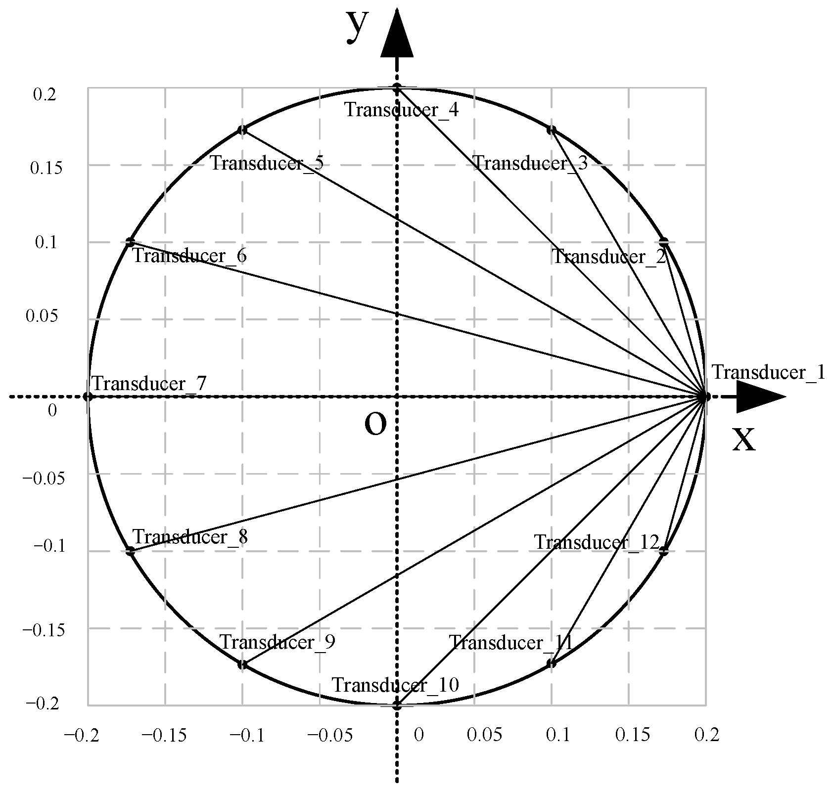
- The number and positions of the transducers.Generally speaking, more transmitters can provide more information for image reconstruction, resulting in more accurate images but possibly with a higher cost of the device and elongated measurement time. As for the transmitters, normally, they are evenly distributed around the periphery of the measurement boundaries to have a balanced interrogation beam coverage over the sensing zone.
- (2)
- The accuracy of the TOF measurement.The relative error of the TOF measurement will lead to the relative error of the temperature measurement.
- (3)
- The state-of-the-art model and algorithm employed in the reconstruction.
3. A Neighboring Cells Regularization Model
3.1. An Analysis of the Conventional Method
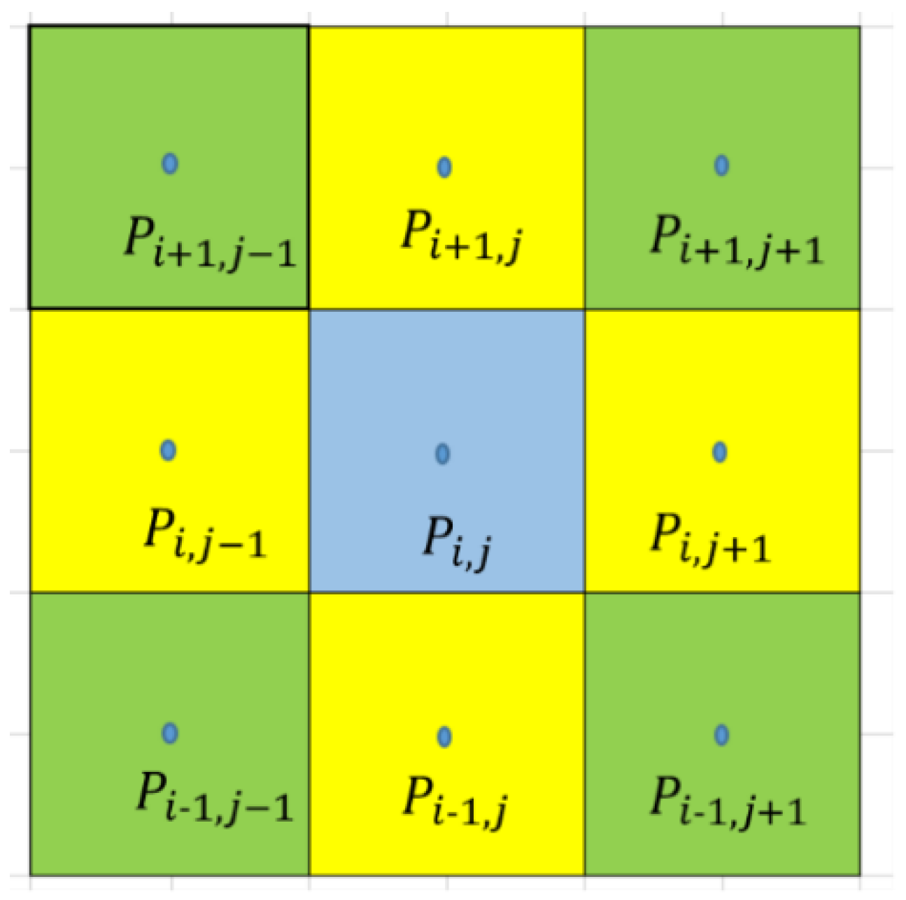
3.2. The Neighboring Cells Regularization Model and Solution Scheme
- (1)
- at the position of ,
- (2)
- at the position of ,
- (3)
- -in the column, which is also the diagonal element of ,
- (4)
- 0 at the other positions.
3.3. Solution of the Model
- (1)
- exists as unique,
- (2)
- If is full-rank, then is the only least square solution of the linear equation .
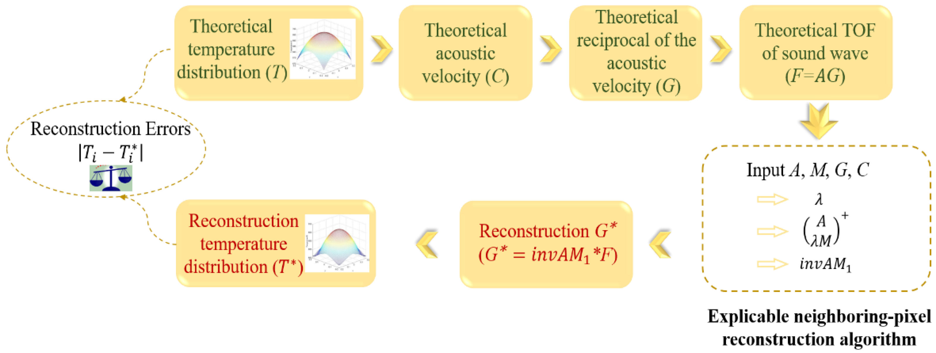
- (1)
- Input , , , and C and assign a value for the regularization parameter .
- (2)
- Calculate , and select its first m raw as .
- (3)
- Calculate the optimal solution .
- (1)
- Equation (35) is used to obtain instead of the commonly used iterative method. Therefore, does not need a particular initialization. This yields a faster speed.
- (2)
- After the size and the positions of the pixels are defined, Matrix is then determined. Similarly, if the setup of the transducers is known, then matrix is also decided. In addition, the value of can be assigned beforehand. Consequently, can also be determined. Because the above can all be precalculated, the solution of the problem can be acquired very quickly.
4. Further Analyses and Simulations
4.1. Error Analysis
4.2. Effect of Parameter
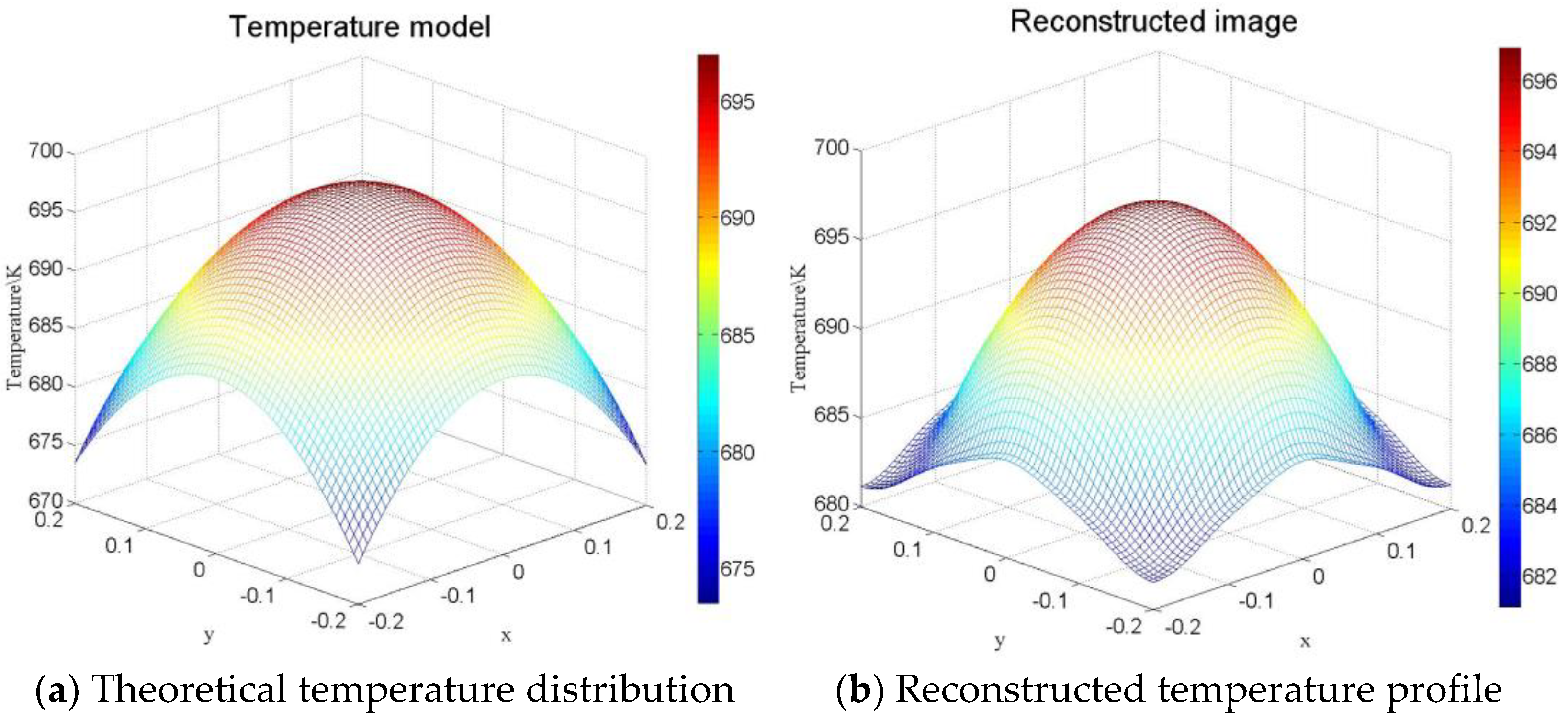
4.3. Simulation
- (1)
- Model I, Central–symmetric temperature distribution,
- (2)
- Model II, Stratified temperature distribution,
- (3)
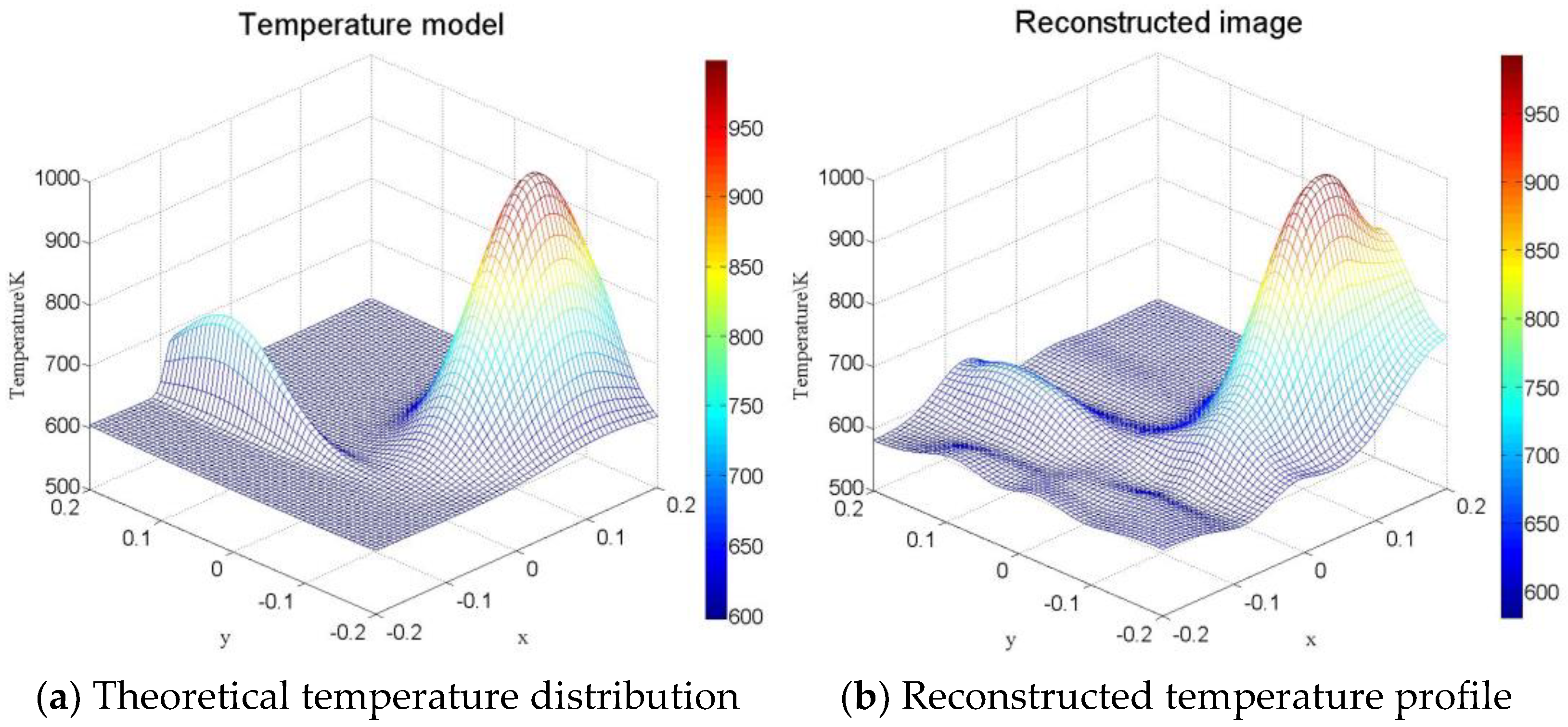
- Model III, Multipeak temperature distribution,
- (4)
- Model IV, Mixed temperature distribution,
5. Conclusions
Author Contributions
Funding
Data Availability Statement
Conflicts of Interest
References
- Barth, M.; Raabe, A. Acoustic tomographic imaging of temperature and flow fields in air. Meas. Sci. Technol. 2011, 22, 035102. [Google Scholar] [CrossRef]
- Holstein, P.; Raabe, A.; Müller, R.; Barth, M.; Mackenzie, D.; Starke, E. Acoustic tomography on the basis of travel-time measurement. Meas. Sci. Technol. 2004, 15, 1420–1428. [Google Scholar] [CrossRef]
- Srinivasan, K.; Sundararajan, T.; Narayanan, S.; Jothi, T.J.S.; Sarma, C.R. Acoustic pyrometry in flames. Measurement 2013, 46, 315–323. [Google Scholar] [CrossRef]
- Lu, J.; Wakai, K.; Takahashi, S.; Shimizu, S. Acoustic computer tomographic pyrometry for two-dimensional measurement of taking into account the effect of refraction of sound wave paths. Meas. Sci. Technol. 2000, 11, 692. [Google Scholar] [CrossRef]
- Zheng, J.; Hua, J.; Tang, Z.; Wang, F. Face detection based on LBP. In Proceedings of the IEEE International Conference on Electronic Measurement & Instruments, Yangzhou, China, 23 January 2018. [Google Scholar]
- Chen, Y.; Hongyu, L.I.; Xia, Z. Electrical Capacitance Tomography Image Reconstruction Algorithm Based on Modified Implicit Formula Landweber Method. Comput. Eng. 2018, 44, 268–273. [Google Scholar]
- Leeuwen, T.V.; Maretzke, S.; Batenburg, K.J. Automatic alignment for three-dimensional tomographic reconstruction. Inverse Probl. 2018, 34, 024004. [Google Scholar] [CrossRef] [Green Version]
- Zhang, S.; Geng, G.; Li, Z.; Zhang, Y. Fast implementation of area integral model SART algorithm based on look-up table. Clust. Comput. 2019, 22, 15195–15203. [Google Scholar] [CrossRef]
- Jin, S.; Du, L. 3-D ionospheric tomography from dense GNSS observations based on an improved two-step iterative algorithm. Adv. Space Res. 2018, 62, 809–820. [Google Scholar] [CrossRef]
- Chun-Fang, L.I.; Zhang, X.F.; Pan, J.H.; Shi, D.F. Modified Simultaneous Algebraic Reconstruction Technique and Its Application in CT from Limited Range. J. Optoelectron. Laser 2002, 13, 726–729. [Google Scholar]
- Hill, E.R.; Xia, W.; Clarkson, M.J.; Desjardins, A.E. Identification and removal of laser-induced noise in photoacoustic imaging using singular value decomposition. Biomed. Opt. Express 2017, 8, 68–77. [Google Scholar] [CrossRef]
- Zhang, J.; Qi, H.; Jiang, D.; He, M.; Ren, Y.; Su, M.; Cai, X. Acoustic tomography of two dimensional velocity field by using meshless radial basis function and modified Tikhonov regularization method. Measurement 2021, 175, 109107. [Google Scholar] [CrossRef]
- Kong, Q.; Jiang, G.; Liu, Y.; Sun, J. 3D high-quality temperature-field reconstruction method in furnace based on acoustic tomography. Appl. Therm. Eng. 2020, 179, 115693. [Google Scholar] [CrossRef]
- Kong, Q.; Jiang, G.; Liu, Y.; Sun, J. 3D temperature distribution reconstruction in furnace based on acoustic tomography. Math. Probl. Eng. 2019, 2019, 1–15. [Google Scholar] [CrossRef] [Green Version]
- Yu, T.; Cai, W. Simultaneous reconstruction of temperature and velocity fields using nonlinear acoustic tomography. Appl. Phys. Lett. 2019, 115, 104104. [Google Scholar] [CrossRef]
- Otero, R.; Lowe, K.T.; Ng, W.F.; Silas, K.A. Coupled velocity and temperature acoustic tomography in heated high subsonic Mach number flows. Meas. Sci. Technol. 2019, 30, 105901. [Google Scholar] [CrossRef]
- Li, J.; Gan, L.; Qin, H. Acoustic velocity tomography for damage detection in concrete 2017. In Proceedings of the 29th Chinese Control and Decision Conference (CCDC), Chongqing, China, 28–30 May 2017; pp. 146–149. [Google Scholar]
- Rao, J.; Yang, J.; Ratassepp, M.; Fan, Z. Multi-parameter reconstruction of velocity and density using ultrasonic tomography based on full waveform inversion. Ultrasonics 2020, 101, 106004. [Google Scholar] [CrossRef]
- Liu, S.; Liu, S.; Ren, T. Ultrasonic tomography based temperature distribution measurement method. Measurement 2016, 94, 671–679. [Google Scholar] [CrossRef]
- Wu, Y.; Zhou, X.; Zhao, L.; Dong, C.; Wang, H. A Method for Reconstruction of Boiler Combustion Temperature Field Based on Acoustic Tomography. Math. Probl. Eng. 2021, 2021, 1–11. [Google Scholar] [CrossRef]
- Chen, Y.; Yan, H. Reconstruction of complex temperature field based on improved Tikhonov regularization. J. Phys. Conf. Ser. 2021, 1754, 012207. [Google Scholar] [CrossRef]
- Liu, S.; Liu, S.; Tong, G. Reconstruction method for inversion problems in an acoustic tomography based temperature distribution measurement. Meas. Sci. Technol. 2017, 28, 115005. [Google Scholar] [CrossRef] [Green Version]
- Wang, H.; Zhou, X.; Yang, Q.; Chen, J.; Dong, C.; Zhao, L. A Reconstruction Method of Boiler Furnace Temperature Distribution Based on Acoustic Measurement. IEEE Trans. Instrum. Meas. 2021, 70, 1–13. [Google Scholar] [CrossRef]
- Bramanti, M.; Salerno, E.A.; Tonazzini, A.; Pasini, S.; Gray, A. An acoustic pyrometer system for tomographic thermal imaging in power plant boilers. IEEE Trans. Instrum. Meas. 1996, 45, 159–167. [Google Scholar] [CrossRef]
- Hua, Y.; Shanhui, W.; Yinggang, Z. Acoustic CT temperature field reconstruction based on adaptive regularization parameter selection. Chin. J. Sci. Instrum. 2012, 33, 103–109. [Google Scholar]
- Avazzadeh, Z.; Heydari, M.; Loghmani, G.B. Numerical solution of Fredholm integral equations of the second kind by using integral mean value theorem. Appl. Math. Model. 2011, 35, 2374–2383. [Google Scholar] [CrossRef]
- Franklin, J.N. Matrix Theory; Courier Corporation: Chelmaford, MA, USA, 2012. [Google Scholar]
- Qiu, Q.; Lu, Z. Matrix Theory and Its Application; China Electric Power Press: Beijing, China, 2018. [Google Scholar]


| Parameter | Number | ||||||||
|---|---|---|---|---|---|---|---|---|---|
| 4 | 5 | 6 | 7 | 8 | 9 | 10 | 11 | 12 | |
| Number of pixels inside the circular zone | 12 | 21 | 32 | 37 | 52 | 69 | 80 | 97 | 112 |
| Parameter | Value | |||||
|---|---|---|---|---|---|---|
| 0.05 | 0.02 | 0.01 | 0.008 | 0.005 | 0.001 | |
| 346.31 | 375.3226 | 380.0822 | 380.6652 | 381.2999 | 381.6919 | |
| Items | Equations | Model Ⅰ | Model Ⅱ | Model Ⅲ | Model Ⅳ |
|---|---|---|---|---|---|
| Maximum absolute error | 0.4323 | 13.1568 | 7.1706 | 9.4499 | |
| Average absolute error | 0.09189 | 1.2261 | 0.9877 | 1.1316 | |
| Maximum relative error | 0.063% | 2.364% | 1.238% | 1.273% | |
| Average relative error | 0.013% | 0.327% | 0.200% | 0.182% | |
| Standard Deviation | 3.1925 × 10⁻⁶ | 8.0440 × 10⁻⁵ | 6.2091 × 10⁻⁷ | 4.57 × 10⁻⁵ |
| Parameter | Value | ||||
|---|---|---|---|---|---|
| 0.01 | 0.0075 | 0.005 | 0.0025 | 0.001 | |
| Maximum absolute error | 62.7365 | 47.26638 | 32.43192 | 18.40133 | 11.22825 |
| Average absolute error | 13.4561 | 10.13784 | 6.88038 | 3.617338 | 1.802721 |
| Maximum relative error | 0.08926 | 0.067117 | 0.045886 | 0.025141 | 0.015198 |
| Average relative error | 0.02266 | 0.017059 | 0.011584 | 0.006055 | 0.002979 |
| Standard deviation | 0.02828 | 0.021248 | 0.014478 | 0.007602 | 0.003837 |
| Parameter | Value | ||||
|---|---|---|---|---|---|
| 0.0005 | 0.0003 | 0.0001 | 0.001 | 0.005 | |
| Maximum absolute error | 11.02863 | 9.889493 | 9.347564 | 13.77893 | 52.1729 |
| Average absolute error | 1.667104 | 1.363348 | 1.160435 | 2.61925 | 11.44429 |
| Maximum relative error | 0.01464 | 0.013525 | 0.012802 | 0.018683 | 0.077785 |
| Average relative error | 0.002745 | 0.002222 | 0.001873 | 0.00437 | 0.019302 |
| Standard deviation | 3.56 × 10⁻³ | 2.98 × 10⁻³ | 2.64 × 10⁻³ | 5.51 × 10⁻³ | 2.42 × 10⁻² |
| The Reconstruction Algorithm | Error in This Paper | Error in the Reference |
|---|---|---|
| Tikhonov-LSSVM (Tikhonov and the least squares support vector machine) in Ref. [24] | Maximum relative error 0.063% | Maximum relative error 0.75% |
| EF-RBFI (radial basis function interpolation method optimized by the evaluation function) in Ref. [25] | Root mean square error 0.0003% | Root mean square error 3.69% |
| Improved Tikhonov Regularization in Ref. [26] | Average relative error 0.013% | Average relative error 1.710% |
| GWO–ABP method (Adaboost.RT based BP neural network algorithm based on Grey wolf optimizer algorithm) in Ref. [27] | Average relative error 0.013% | Average relative error 1.16% |
| LQ-SVD (logarithmic–quadratic radial basis function and singular value decomposition algorithm) in Ref. [28] | Root mean square error 0.0003% | Root mean square error 3.0617% |
Publisher’s Note: MDPI stays neutral with regard to jurisdictional claims in published maps and institutional affiliations. |
© 2022 by the authors. Licensee MDPI, Basel, Switzerland. This article is an open access article distributed under the terms and conditions of the Creative Commons Attribution (CC BY) license (https://creativecommons.org/licenses/by/4.0/).
Share and Cite
Qiu, Q.; Zhou, W.; Zhao, Q.; Liu, S. An Explicable Neighboring-Pixel Reconstruction Algorithm for Temperature Distribution by Acoustic Tomography. Energies 2022, 15, 3118. https://doi.org/10.3390/en15093118
Qiu Q, Zhou W, Zhao Q, Liu S. An Explicable Neighboring-Pixel Reconstruction Algorithm for Temperature Distribution by Acoustic Tomography. Energies. 2022; 15(9):3118. https://doi.org/10.3390/en15093118
Chicago/Turabian StyleQiu, Qirong, Wanting Zhou, Qing Zhao, and Shi Liu. 2022. "An Explicable Neighboring-Pixel Reconstruction Algorithm for Temperature Distribution by Acoustic Tomography" Energies 15, no. 9: 3118. https://doi.org/10.3390/en15093118
APA StyleQiu, Q., Zhou, W., Zhao, Q., & Liu, S. (2022). An Explicable Neighboring-Pixel Reconstruction Algorithm for Temperature Distribution by Acoustic Tomography. Energies, 15(9), 3118. https://doi.org/10.3390/en15093118