Positive Torque Modulation Method and Key Technology of Conventional Beam Pumping Unit

Abstract

The large fluctuation of net torque and the existence of negative torque on the crank output shaft of the beam pumping unit are the decisive factors leading to its low efficiency and high energy consumption. The conventional pumping unit CYJ10-4.2-53HF was selected as the study object on the basis of the fixed shaft secondary balance principle and the positive torque modulation scheme was first proposed according to the following secondary balance principle based on the linkage. The kinematics analysis of the suspension point and the secondary incremental velocity mechanism were carried out using the theory of rigid body plane kinematics. The force analysis of each moving part of the pumping unit was carried out, the net torque expression of the crank output shaft was obtained, and an example calculation was performed. The positive torque beam pumping unit was developed and tested in a field test. The tests showed that the positive torque beam pumping unit was able to fully realize positive torque operation under field well conditions, with a power saving rate of 23.73% and a 14.5% increase in system efficiency, and that the reliability of the pumping unit meets the requirements for field application.

1. Introduction

Conventional beam pumping units are widely used in oilfields due to their advantages of simple structure, high reliability, and convenient maintenance [1,2,3]. However, the structural characteristics of conventional beam pumping units determine their poor balance effect, large net torque fluctuation of the crank output shaft and existence of negative torque, low efficiency, and high energy consumption [4,5,6,7]. The large net torque fluctuation of the crank output shaft and the existence of negative torque are the decisive factors leading to its low efficiency and high energy consumption [8,9]. In response to this problem, many scholars and pumping machine manufacturers both at home and abroad have developed a variety of new energy-saving pumping units [10,11,12] which have achieved certain energy-saving effects; however, most of the new pumping units are not yet able to solve the problem of negative torque in the crank output shaft, and the disadvantages of the new energy-saving pumping machines in terms of reliability and maintenance management restrict their development [13,14,15,16,17,18]. On the other hand, the number of beam pumping machines accounts for more than 80% of all pumping units [3,19], and it is impossible to replace all of them in a short time from the perspective of resource utilization and economic cost. Therefore, it is a more reasonable solution to implement a low-cost transformation of conventional beam pumping units by modulating the negative torque of the crank output shaft to positive torque. In this paper, a positive torque modulation scheme for a conventional beam pumping unit, CYJ10-4.2-53HF, is proposed for the first time based on the principle of secondary balancing of the following linkage rod, and the proposed method is applied in the field. After the kinematics and dynamics of the transformed pumping unit were analyzed, a prototype was manufactured and verified in the field.

2. Modulation Principle and Method

2.1. Modulation Method

Based on the principle of fixed shaft secondary balance, the crank output shaft positive torque modulation method and structure of conventional beam pumping unit are shown in Figure 1 and Figure 2. The secondary balance system mainly includes the speed increaser box and the secondary balance weight, and the original connecting rod is replaced by a connecting rod frame which is connected to the cross beam at one end and the speed increase gearbox at the other end. The input shaft of the speed increase gearbox is equipped with a large gear and the output shaft with a small gear; the transmission ratio of the large gear and the small gear is 1:2. The input end of the input shaft of the speed increase gearbox is fixed together with the large crank and the output end of the output shaft of the speed increase gearbox is connected to the secondary balance weight.

2.2. Analysis of Working Process and Balancing Effect

When the pumping unit works, the original movement form of the connecting rod in the plane is replaced by the speed increase gearbox and the connecting rod frame, as they are fixed together. The secondary balance weight is fixed on the output shaft of the speed increase gearbox; thus, the secondary balance follows the speed increase gearbox and the connecting rod frame together to move in space plane motion and rotate around the output shaft. This positive torque modulation method can be called as the secondary balance based on following the connecting rod. The mass and motion inertia force of secondary balancing adds a dynamic balancing block to the big crank to play the role of primary balancing, and it can be said that the secondary balancing based on the connecting rod with the action plays the role of both secondary balancing and of primary balancing, which is conducive to reducing the weight of primary balancing and saving steel.

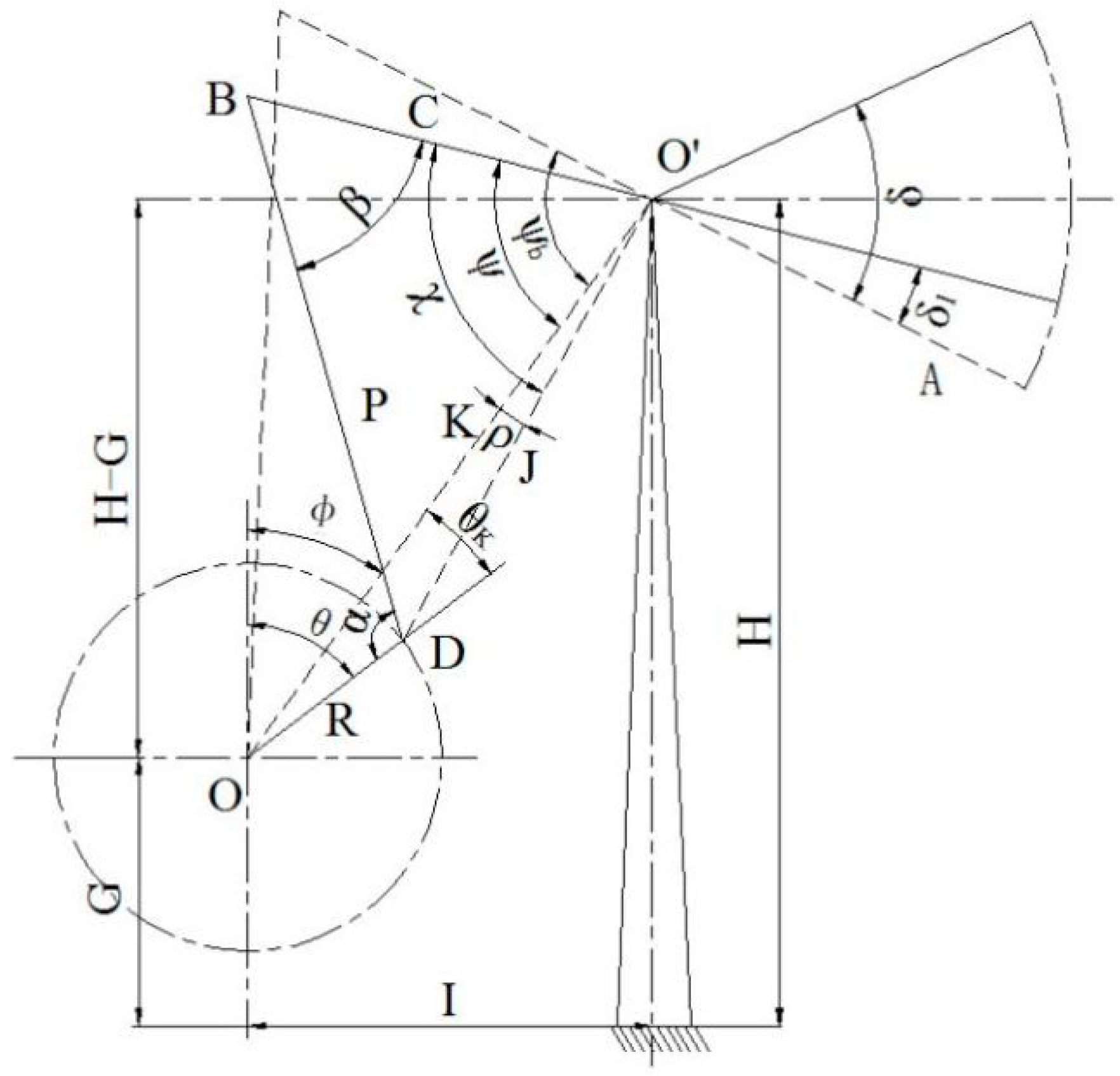
3. Kinematic Analysis

3.1. Kinematic Analysis of the Suspension Point

A motion analysis sketch of the modified pumping unit suspension point is shown in Figure 3 [20,21,22,23], and can be obtained from Figure 3:

$$\varphi =\pm \arctan (\frac{I}{H-G})$$

(1)

$${\theta }_k=\theta -\varphi$$

(2)

$$\psi =\chi -\rho$$

(3)

$${\psi }_b=\arccos (\frac{C^2+K^2-{(P+R)}^2}{2CK})$$

(4)

$${\psi }_t=\arccos (\frac{C^2+K^2-{(P-R)}^2}{2CK})$$

(5)

$$\alpha =\pm (\beta +\psi )-{\theta }_k=\pm (\beta +\chi -\rho )-\theta +\varphi$$

(6)

The swing angle of the beam is ${\delta }_i$

$${\delta }_i={\psi }_b-\psi$$

(7)

The displacement of the suspension point is

$$S_i=A{\delta }_i$$

(8)

The angular velocity ${\omega }_b$ of the beam is

$${\omega }_b=\frac{R}{C}\omega \frac{\sin \alpha }{\sin \beta }$$

(9)

where $\omega$ is the angular velocity of crank rotation, s⁻¹.

The velocity v (m/s) of the beam is

$$v=A{\omega }_b=\frac{A}{C}R\omega \frac{\sin \alpha }{\sin \beta }$$

(10)

The angular acceleration, ${\epsilon }_{\mathrm{b}}$, of the beam can be obtained from the derivative of the angular velocity, ${\omega }_{\mathrm{b}}$, with respect to the time, t. The acceleration at the suspension point is a (m/s²):

$$a=A{\epsilon }_b=\frac{ARK}{CP}{\omega }^2\frac{\sin \beta \cos \alpha \sin \psi -\frac{R}{C}\sin \alpha \cos \beta \sin {\theta }_k}{{\sin }^3\beta }$$

(11)

Figure 3. The motion analysis sketch of the modified pumping unit suspension point.

Figure 3. The motion analysis sketch of the modified pumping unit suspension point.

3.2. Kinematic Analysis of Secondary Speed Increasing Mechanism

3.2.1. Angular Velocity Analysis

A schematic diagram of the secondary balance motion analysis is shown in Figure 4. The angular velocity, ${\omega }_1$ (rad/s), of the connecting rod BD is

$${\omega }_1=\frac{v_{\mathrm{D}}}{DE}=\frac{R\omega \sin (\alpha -\beta )}{P\sin \beta }$$

(12)

Therefore, the angular acceleration, ${\alpha }_1$ (rad/s²), of the connecting rod BD is

$${\alpha }_1=\frac{\mathrm{d}{\omega }_1}{\mathrm{dt}}=\frac{RK{\omega }^2(C\sin \beta \sin \psi \cos (\alpha -\beta )-R\sin \alpha \sin {\theta }_{\mathrm{k}})}{C{P}^2{\sin }^3\beta }$$

(13)

The velocity at the gear meshing point G is

$$v_{\mathrm{G}}=\omega \cdot OG=\omega \sqrt{R^2+r_1{}^2-2R{r}_1\cos \alpha }$$

(14)

The angular velocity, ${\omega }_2$, of the pinion is

$$\begin{array}{l}{\omega }_2=\frac{v_G}{GH}=\omega -\frac{R\omega \cos \alpha }{r_1}+\frac{R\omega (r_1+r_2)\sin (\alpha -\beta )}{2r_{1}P\sin \beta }+\frac{RP\omega ({\sin }^2\alpha -{\sin }^2\beta )}{2r_1(r_1+r_2)\sin \beta \sin (\alpha -\beta )}\\ +\frac{R\omega {(P-r_1-r_2)}^2\sin (\alpha -\beta )}{2r_1(r_1+r_2)P\sin \beta }-\frac{R\omega \sin \alpha \cos \beta (P-r_1-r_2)}{r_1(r_1+r_2)\sin \beta }\end{array}$$

(15)

where r₁ and r₂ denote the radii of the reference circle of the large gear and the pinion, respectively. The angular acceleration, ${\alpha }_2$, of the small crank is obtained by deriving the angular velocity, ${\omega }_2$, of the small crank with respect to time, t.

Figure 4. Schematic diagram of secondary balance motion analysis.

Figure 4. Schematic diagram of secondary balance motion analysis.

3.2.2. Analysis of Secondary Balance Acceleration

The acceleration of the secondary balance is analyzed as shown in Figure 5. For the center point, F, of the pinion rotating together with the connecting rod BD, the instantaneous center of point F is point E, and ${\mathit{a}}_{\mathrm{F}}^{\mathrm{n}}$ and ${\mathit{a}}_{\mathrm{F}}^{\mathrm{t}}$ are the normal and tangential acceleration of point F, respectively. Therefore, the acceleration of point F is

$${\mathit{a}}_{\mathrm{F}}={\mathit{a}}_{\mathrm{F}}^{\mathrm{n}}+{\mathit{a}}_{\mathrm{F}}^{\mathrm{t}}$$

(16)

$$\begin{array}{l}{\mathit{a}}_{\mathrm{F}}^{\mathrm{n}}={\omega }_1^2\cdot EF\\ =\frac{R^2{\omega }^2{\sin }^2(\alpha -\beta )}{P^2{\sin }^2\beta }\sqrt{\frac{P^2{\sin }^2\alpha }{{\sin }^2(\alpha -\beta )}+{(P-r_1-r_2)}^2-\frac{2P\sin \alpha \cos \beta (P-r_1-r_2)}{\sin (\alpha -\beta )}}\end{array}$$

(17)

$$\begin{array}{l}{\mathit{a}}_{\mathrm{F}}^{\mathrm{t}}={\alpha }_1\cdot EF=\frac{R{\omega }^2\sin \beta \cos (\alpha -\beta )(\frac{\mathrm{d}\alpha }{\mathrm{d}\theta }-\frac{\mathrm{d}\beta }{\mathrm{d}\theta })-R{\omega }^2\sin (\alpha -\beta )\cos \beta \frac{\mathrm{d}\beta }{\mathrm{d}\theta }}{P{\sin }^2\beta }\cdot \\ \sqrt{\frac{P^2{\sin }^2\alpha }{{\sin }^2(\alpha -\beta )}+{(P-r_1-r_2)}^2-\frac{2P\sin \alpha \cos \beta (P-r_1-r_2)}{\sin (\alpha -\beta )}}\end{array}$$

(18)

The mass center of the secondary balance block and the secondary balance crank is I; if $\mathrm{IF}=r$, list the acceleration of point I using point F as the base point:

$${\mathit{a}}_{\mathrm{I}}={\mathit{a}}_{\mathrm{F}}+{\mathit{a}}_{\mathrm{IF}}^{\mathrm{t}}+{\mathit{a}}_{\mathrm{IF}}^{\mathrm{n}}={\mathit{a}}_{\mathrm{F}}^{\mathrm{n}}+{\mathit{a}}_{\mathrm{F}}^{\mathrm{t}}+{\mathit{a}}_{\mathrm{IF}}^{\mathrm{t}}+{\mathit{a}}_{\mathrm{IF}}^{\mathrm{n}}$$

(19)

$$\mathrm{where} a_{\mathrm{IF}}^{\mathrm{t}}={\alpha }_{2}r, a_{\mathrm{IF}}^{\mathrm{n}}={\omega }_2^{2}r$$

(20)

$$\angle \mathrm{EFM}=\frac{\pi }{2}-{\tau }^{\prime }-\epsilon -\beta -\gamma +\angle \mathrm{DFE}$$

(21)

$$\frac{\mathrm{d}\epsilon }{\mathrm{dt}}=\frac{\mathrm{d}\epsilon }{\mathrm{d}\theta }\frac{\mathrm{d}\theta }{\mathrm{dt}}=\frac{\mathrm{d}\epsilon }{\mathrm{d}\theta }\omega ={\omega }_2$$

(22)

$$\begin{array}{l}\epsilon ={\displaystyle {\int }_0^{\theta }\frac{{\omega }_2}{\omega }}d\theta \\ ={\displaystyle {\int }_0^{\theta }\left. [\begin{array}{l}\frac{r_1-R\cos \alpha }{r_1}+\frac{R{(r_1+r_2)}^2{\sin }^2(\alpha -\beta )+R{P}^2{\sin }^2\alpha -R{P}^2{\sin }^2\beta }{2r_1(r_1+r_2)P\sin \beta \sin (\alpha -\beta )}\\ +\frac{R{(P-r_1-r_2)}^2{\sin }^2(\alpha -\beta )-2RP\sin \alpha \cos \beta \sin (\alpha -\beta )(P-r_1-r_2)}{2r_1(r_1+r_2)P\sin \beta \sin (\alpha -\beta )}\end{array}\right]}d\theta \end{array}$$

(23)

Decomposing Equation (19) in the t and n directions, respectively,

$$a_{\mathrm{I}}^{\mathrm{t}}=a_{\mathrm{F}}^{\mathrm{n}}\cos \angle \mathrm{EFM}+a_{\mathrm{F}}^{\mathrm{t}}\sin \angle \mathrm{EFM}+a_{\mathrm{IF}}^{\mathrm{n}}, a_{\mathrm{I}}^{\mathrm{n}}=-a_{\mathrm{F}}^{\mathrm{n}}\sin \angle \mathrm{EFM}+a_{\mathrm{F}}^{\mathrm{t}}\cos \angle \mathrm{EFM}+a_{\mathrm{IF}}^{\mathrm{t}}$$

(24)

Substituting Equations (20), (21) and (23) into (24), respectively, $a_{\mathrm{I}}^{\mathrm{t}}$, $a_{\mathrm{I}}^{\mathrm{n}}$ of the pinion center F can be obtained.

Figure 5. Acceleration analysis of secondary balance of the pumping unit after transformation: (a) complete analysis of the secondary balance acceleration; (b) partial enlarged analysis of the secondary balance accelerations.

Figure 5. Acceleration analysis of secondary balance of the pumping unit after transformation: (a) complete analysis of the secondary balance acceleration; (b) partial enlarged analysis of the secondary balance accelerations.

4. Torque Analysis on the Output Shaft of Gearbox

4.1. Force Analysis of Secondary Balance

The force analysis diagram of the positive torque beam pumping unit is shown in Figure 6. From the kinematic analysis of the secondary speed increment mechanism and D’Alembert’s theorem of the mass system, the force analysis sketch of the secondary balance is shown in Figure 7 after adding the inertia force of the mass, I. Where, $F_{\mathrm{Ft}}$, $F_{\mathrm{Fn}}$ and $M_{\mathrm{F}}$ are the forces and moment of the pinion shaft acting on the secondary equilibrium along the t and n directions, respectively, $F_{\mathrm{I}}^{\mathrm{t}}$, $F_{\mathrm{I}}^{\mathrm{n}}$, and $M_{\mathrm{II}}$ are the imaginary added inertia forces and moment of inertia corresponding to the acceleration $a_{\mathrm{I}}^{\mathrm{t}}$, $a_{\mathrm{I}}^{\mathrm{n}}$ and angular acceleration, ${\alpha }_2$, of the secondary balance mass I, respectively.

Figure 6. Force analysis diagram of the whole pumping unit.

Figure 6. Force analysis diagram of the whole pumping unit.

Figure 7. Force analysis diagram of the secondary balance.

Figure 7. Force analysis diagram of the secondary balance.

$$F_{\mathrm{I}}^{\mathrm{t}}=m_{\mathrm{e}}{a}_{\mathrm{I}}^{\mathrm{t}}, F_{\mathrm{I}}^{\mathrm{n}}=m_{\mathrm{e}}{a}_{\mathrm{I}}^{\mathrm{n}}, M_{\mathrm{II}}=J_{\mathrm{e}}{\alpha }_2$$

(25)

Based on D’Alembert’s principle for the mass system, the force balance equations are listed as follows:

$$\left\{\begin{array}{l}\sum F_{\mathrm{n}}=0:F_{\mathrm{Fn}}+W_{\mathrm{e}}\cos ({\tau }^{\prime }+\epsilon )-F_{\mathrm{I}}^{\mathrm{n}}=0\\ \sum F_{\mathrm{t}}=0:W_{\mathrm{e}}\sin ({\tau }^{\prime }+\epsilon )-F_{\mathrm{Ft}}-F_{\mathrm{I}}^{\mathrm{t}}=0\\ \sum M_{\mathrm{F}}=0:M_{\mathrm{F}}+W_{\mathrm{e}}r\sin ({\tau }^{\prime }+\epsilon )-F_{\mathrm{I}}^{\mathrm{t}}r-M_{\mathrm{II}}=0\end{array}\right.$$

(26)

After solving from the system of Equation (26) and bringing in Equation (25) we obtain

$$F_{\mathrm{Fn}}=m_{\mathrm{e}}{a}_{\mathrm{I}}^{\mathrm{n}}-m_{\mathrm{e}}g\cos ({\tau }^{\prime }+\epsilon )$$

(27)

$$F_{\mathrm{Ft}}=m_{\mathrm{e}}g\sin ({\tau }^{\prime }+\epsilon )-m_{\mathrm{e}}{a}_{\mathrm{I}}^{\mathrm{t}}$$

(28)

$$M_{\mathrm{F}}=m_{\mathrm{e}}{a}_{\mathrm{I}}^{\mathrm{t}}r+J_{\mathrm{e}}{\alpha }_2-m_{\mathrm{e}}gr\sin ({\tau }^{\prime }+\epsilon )$$

(29)

Projecting $F_{\mathrm{Ft}}$, $F_{\mathrm{Fn}}$ to the x and y axes, respectively, determine $F_{\mathrm{F}x}$, $F_{\mathrm{F}y}$:

$$F_{\mathrm{F}x}=m_{\mathrm{e}}{a}_{\mathrm{I}}^{\mathrm{n}}\sin ({\tau }^{\prime }+\epsilon )-m_{\mathrm{e}}{a}_{\mathrm{I}}^{\mathrm{t}}\cos ({\tau }^{\prime }+\epsilon )$$

(30)

$$F_{\mathrm{F}y}=m_{\mathrm{e}}g-m_{\mathrm{e}}{a}_{\mathrm{I}}^{\mathrm{n}}\cos ({\tau }^{\prime }+\epsilon )-m_{\mathrm{e}}{a}_{\mathrm{I}}^{\mathrm{t}}\sin ({\tau }^{\prime }+\epsilon )$$

(31)

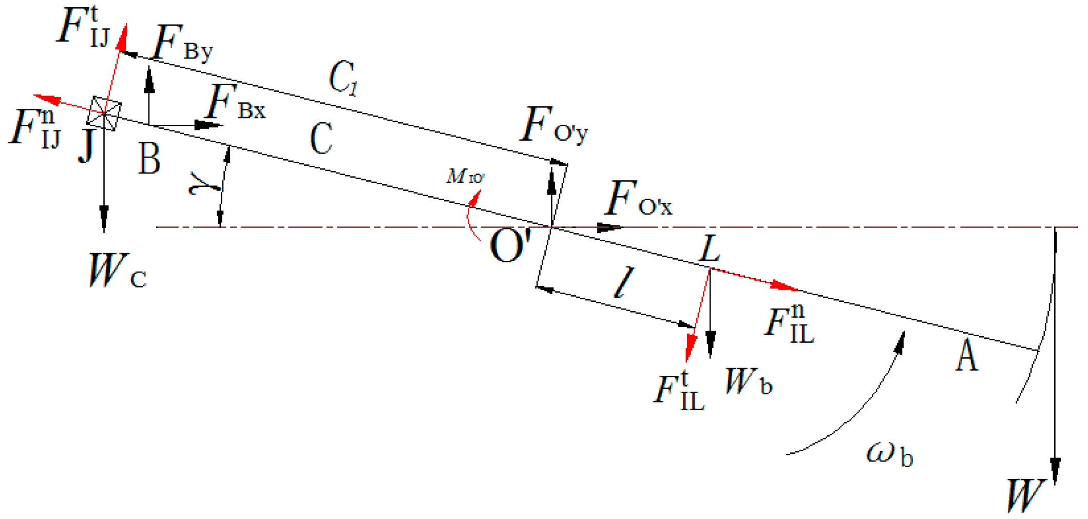
4.2. Force Analysis of the Beam

The force analysis diagram of the beam is shown in Figure 8; based on D’Alembert’s principle for mass systems, the system of force balance equations is listed below:

Figure 8. Force analysis of the beam.

Figure 8. Force analysis of the beam.

$$\left\{\begin{array}{l}\sum F_x=0:F_{\mathrm{O}\prime x}+F_{\mathrm{B}x}+F_{\mathrm{IJ}}^{\mathrm{t}}\sin \gamma +F_{\mathrm{IL}}^{\mathrm{n}}\cos \gamma -F_{\mathrm{IJ}}^{\mathrm{n}}\cos \gamma -F_{\mathrm{IL}}^{\mathrm{t}}\sin \gamma =0\\ \sum F_y=0:F_{\mathrm{O}\prime y}+F_{\mathrm{B}y}+F_{\mathrm{IJ}}^{\mathrm{t}}\cos \gamma +F_{\mathrm{IJ}}^{\mathrm{n}}\sin \gamma +F_{\mathrm{IL}}^{\mathrm{n}}\sin \gamma -F_{\mathrm{IL}}^{\mathrm{t}}\cos \gamma -W_{\mathrm{c}}-W_{\mathrm{b}}-W=0\\ \sum M_{\mathrm{O}\prime }=0:W_{\mathrm{c}}{C}_1\cos \gamma -WA-W_{\mathrm{b}}l\cos \gamma -F_{\mathrm{B}x}C\sin \gamma -F_{\mathrm{B}y}C\cos \gamma -F_{\mathrm{IJ}}^{\mathrm{t}}{C}_1\\ -F_{\mathrm{IL}}^{\mathrm{t}}l-M_{\mathrm{I}\mathrm{O}\prime }=0\end{array}\right.$$

(32)

where $\gamma =\chi -\rho -(\frac{\pi }{2}-\phi )=\chi +\phi -\rho -\frac{\pi }{2}$, $F_{\mathrm{IL}}^{\mathrm{t}}=\frac{W_{\mathrm{b}}}{g}{\epsilon }_{\mathrm{b}}l$, $F_{\mathrm{IL}}^{\mathrm{n}}=\frac{W_{\mathrm{b}}}{g}{\omega }_{\mathrm{b}}^{2}l$, $F_{\mathrm{IJ}}^{\mathrm{t}}=\frac{W_{\mathrm{c}}}{g}{\epsilon }_{\mathrm{b}}{C}_1$, $F_{\mathrm{IJ}}^{\mathrm{n}}=\frac{W_{\mathrm{c}}}{g}{\omega }_{\mathrm{b}}^2{C}_1$, $M_{\mathrm{I}\mathrm{O}\prime }=J_{\mathrm{b}}{\epsilon }_{\mathrm{b}}=(\frac{W_{\mathrm{b}}}{g}{l}^2+\frac{W_{\mathrm{c}}}{g}{C}_1{}^2){\epsilon }_b$.

The four unknowns are $F_{\mathrm{O}\prime x}$, $F_{\mathrm{O}\prime y}$, $F_{\mathrm{B}x}$, $F_{\mathrm{B}y}$.

4.3. Force Analysis of the Linkage-Speed Increase Gearbox

Because the linkage and the speed increase gearbox are welded together, they can be analyzed as a single unit in the force analysis; the force diagram is shown in Figure 9. It can be drawn from the geometric relationship on Figure 9:

$$\eta =\angle EFJ=\pi -\angle DFE-\angle JFB=\pi -\angle DFE-(\frac{\pi }{2}-\beta -\gamma )=\beta +\chi +\phi -\rho -\angle DFE$$

(33)

$$\zeta =\pi -\angle DFE-\eta =\pi -(\beta +\chi +\phi -\rho -\angle DFE)-\angle DFE=\pi +\rho -\beta -\chi -\phi$$

(34)

Based on D’Alembert’s principle, the system of force balance equations is listed as follows:

$$\{\begin{array}{l}\sum F_x=0:F_{\mathrm{D}x}-F_{\mathrm{B}x}{}^{\prime }-F_{\mathrm{F}x}{}^{\prime }-F_{\mathrm{IF}}^{\mathrm{t}}\cos \eta -F_{\mathrm{IF}}^{\mathrm{n}}\sin \eta =0\\ \sum F_y=0:F_{\mathrm{D}y}+F_{\mathrm{IF}}^{\mathrm{t}}\sin \eta -F_{\mathrm{IF}}^{\mathrm{n}}\cos \eta -F_{\mathrm{B}y}{}^{\prime }-F_{\mathrm{F}y}{}^{\prime }-W_{\mathrm{f}}=0\\ \sum M_{\mathrm{D}}=0:F_{\mathrm{B}x}{}^{\prime }P\cos \zeta +F_{\mathrm{B}y}{}^{\prime }P\sin \zeta +F_{\mathrm{F}x}{}^{\prime }(r_1+r_2)\cos \zeta +(F_{\mathrm{F}y}{}^{\prime }+W_{\mathrm{f}}\left)\right(r_1+r_2)\sin \zeta \\ +F_{\mathrm{IF}}^{\mathrm{t}}(r_1+r_2\left)\cos \right(\eta +\zeta )+F_{\mathrm{IF}}^{\mathrm{n}}(r_1+r_2\left)\sin \right(\eta +\zeta )-M_{\mathrm{IF}}=0\\ \sum M_{\mathrm{F}}=0:F_{\mathrm{B}x}{}^{\prime }(P-r_1-r_2)\cos \zeta +F_{\mathrm{B}y}{}^{\prime }(P-r_1-r_2)\sin \zeta +F_{\mathrm{D}x}(r_1+r_2)\cos \zeta \\ +F_{\mathrm{D}y}(r_1+r_2)\sin \zeta -M_{\mathrm{IF}}=0\\ \sum M_{\mathrm{B}}=0:F_{\mathrm{D}x}P\cos \zeta +F_{\mathrm{D}y}P\sin \zeta -F_{\mathrm{F}x}{}^{\prime }(P-r_1-r_2)\cos \zeta -(F_{\mathrm{F}y}{}^{\prime }+W_{\mathrm{f}}\left)\right(P-r_1-r_2)\sin \zeta \\ -F_{\mathrm{IF}}^{\mathrm{t}}(P-r_1-r_2\left)\cos \right(\eta +\zeta )-F_{\mathrm{IF}}^{\mathrm{n}}(P-r_1-r_2\left)\sin \right(\eta +\zeta )-M_{\mathrm{IF}}=0\end{array}$$

(35)

where $F_{\mathrm{IF}}^{\mathrm{t}}=\frac{W_{\mathrm{f}}}{g}{\alpha }_1\cdot EF$, $F_{\mathrm{IF}}^{\mathrm{n}}=\frac{W_{\mathrm{f}}}{g}{\omega }_1^2\cdot EF$, $M_{\mathrm{IF}}=J_{\mathrm{f}}{\alpha }_1$.

The five unknowns are $F_{\mathrm{B}x}{}^{\prime }$, $F_{\mathrm{B}y}{}^{\prime }$, $F_{\mathrm{D}x}$, $F_{\mathrm{D}y}$ and $M_{\mathrm{D}}$.

Figure 9. Force diagram of the linkage-speed increase gearbox: (a) complete analysis diagram of linkage-speed increase gearbox; (b) partial enlarged analysis diagram of linkage-speed increase gearbox.

Figure 9. Force diagram of the linkage-speed increase gearbox: (a) complete analysis diagram of linkage-speed increase gearbox; (b) partial enlarged analysis diagram of linkage-speed increase gearbox.

4.4. Force Analysis of the Large Crank

The force analysis of the large crank is shown in Figure 10. Based D’Alembert’s principle, the system of force balance equations is listed as follows:

$$\left\{\begin{array}{l}\sum F_x=0:F_{\mathrm{O}x}+F_{\mathrm{IM}}^{\mathrm{t}}\sin (\theta -\tau )-F_{\mathrm{D}x}{}^{\prime }=0\\ \sum F_y=0:F_{\mathrm{O}y}+F_{\mathrm{IM}}^{\mathrm{t}}\cos (\theta -\tau )-F_{\mathrm{D}y}{}^{\prime }-W_{\mathrm{d}}=0\\ \sum M_{\mathrm{O}}=0:M-M_{\mathrm{D}}{}^{\prime }+F_{\mathrm{D}x}{}^{\prime }R\cos \theta -F_{\mathrm{D}y}{}^{\prime }R\sin \theta -W_{\mathrm{d}}a\sin (\theta -\tau )=0\end{array}\right.$$

(36)

where $F_{\mathrm{IM}}^{\mathrm{t}}=\frac{W_{\mathrm{d}}}{g}{\omega }^{2}b$.

The five unknowns are $F_{\mathrm{O}x}$, $F_{\mathrm{O}y}$, $F_{\mathrm{D}x}$, $F_{\mathrm{D}y}$ and $M_D{}^{\prime }$.

Figure 10. Force analysis of the large crank balance weight.

Figure 10. Force analysis of the large crank balance weight.

4.5. Solving the Force Equations

The system of force analysis Equation (32) of the beam is organized to obtain

$$\left\{\begin{array}{l}{F}_{\mathrm{O}\prime x}+F_{\mathrm{B}x}=-F_{\mathrm{IJ}}^{\mathrm{t}}\sin \gamma -F_{\mathrm{IL}}^{\mathrm{n}}\cos \gamma +F_{\mathrm{IJ}}^{\mathrm{n}}\cos \gamma +F_{\mathrm{IL}}^{\mathrm{t}}\sin \gamma \\ F_{\mathrm{O}\prime y}+F_{\mathrm{B}y}=-F_{\mathrm{IJ}}^{\mathrm{t}}\cos \gamma -F_{\mathrm{IJ}}^{\mathrm{n}}\sin \gamma -F_{\mathrm{IL}}^{\mathrm{n}}\sin \gamma +F_{\mathrm{IL}}^{\mathrm{t}}\cos \gamma +W_{\mathrm{c}}+W_{\mathrm{b}}+W\\ F_{\mathrm{B}x}C\sin \gamma +F_{\mathrm{B}y}C\cos \gamma =W_{\mathrm{c}}{C}_1\cos \gamma -WA-W_{\mathrm{b}}l\cos \gamma -F_{\mathrm{IJ}}^{\mathrm{t}}{C}_1-F_{\mathrm{IL}}^{\mathrm{t}}l-M_{\mathrm{I}\mathrm{O}\prime }\end{array}\right.$$

(37)

Due to $F_{\mathrm{D}x}{}^{\prime }=F_{\mathrm{D}x}$, $F_{\mathrm{B}y}{}^{\prime }=F_{\mathrm{B}y}$, $F_{\mathrm{F}x}{}^{\prime }=F_{\mathrm{F}x}$, $F_{\mathrm{F}y}{}^{\prime }=F_{\mathrm{F}y}$, $M_F{}^{\prime }=M_F$, the system of force analysis Equation (35) for the linkage-speed increase gearbox is sorted to obtain

$$\{\begin{array}{l}{F}_{\mathrm{D}x}-F_{\mathrm{B}x}=F_{\mathrm{IF}}^{\mathrm{t}}\cos \eta +F_{\mathrm{IF}}^{\mathrm{n}}\sin \eta +F_{\mathrm{F}x}\\ F_{\mathrm{D}y}-F_{\mathrm{B}y}=-F_{\mathrm{IF}}^{\mathrm{t}}\sin \eta +F_{\mathrm{IF}}^{\mathrm{n}}\cos \eta +F_{\mathrm{F}y}+W_{\mathrm{f}}\\ F_{\mathrm{B}x}P\cos \zeta +F_{\mathrm{B}y}P\sin \zeta =-F_{\mathrm{F}x}(r_1+r_2)\cos \zeta -(F_{\mathrm{F}y}+W_{\mathrm{f}}\left)\right(r_1+r_2)\sin \zeta \\ -F_{\mathrm{IF}}^{\mathrm{t}}(r_1+r_2\left)\cos \right(\eta +\zeta )-F_{\mathrm{IF}}^{\mathrm{n}}(r_1+r_2\left)\sin \right(\eta +\zeta )+M_{\mathrm{IF}}\\ F_{\mathrm{B}x}(P-r_1-r_2)\cos \zeta +F_{\mathrm{B}y}(P-r_1-r_2)\sin \zeta +F_{\mathrm{D}x}(r_1+r_2)\cos \zeta +F_{\mathrm{D}y}(r_1+r_2)\sin \zeta =M_{\mathrm{IF}}\\ F_{\mathrm{D}x}P\cos \zeta +F_{\mathrm{D}y}P\sin \zeta =F_{\mathrm{F}x}(P-r_1-r_2)\cos \zeta +(F_{\mathrm{F}y}{}^{\prime }+W_{\mathrm{f}}\left)\right(P-r_1-r_2)\sin \zeta \\ +F_{\mathrm{IF}}^{\mathrm{t}}(P-r_1-r_2\left)\cos \right(\eta +\zeta )+F_{\mathrm{IF}}^{\mathrm{n}}(P-r_1-r_2\left)\sin \right(\eta +\zeta )+M_{\mathrm{IF}}\end{array}$$

(38)

Due to $F_{\mathrm{D}x}{}^{\prime }=F_{\mathrm{D}x}$, $F_{\mathrm{D}y}{}^{\prime }=F_{\mathrm{D}y}$, $M_{\mathrm{D}}{}^{\prime }=M_{\mathrm{D}}=2M_{\mathrm{F}}$, the equation system of the large crank balance force analysis (36) is organized to obtain

$$\left\{\begin{array}{l}{F}_{\mathrm{O}x}-F_{\mathrm{D}x}=-F_{\mathrm{IM}}^{\mathrm{t}}\sin (\theta -\tau )\\ F_{\mathrm{O}y}-F_{\mathrm{D}y}=W_{\mathrm{d}}-F_{\mathrm{IM}}^{\mathrm{t}}\cos (\theta -\tau )\\ M+F_{\mathrm{D}x}R\cos \theta -F_{\mathrm{D}y}R\sin \theta =W_{\mathrm{d}}a\sin (\theta -\tau )+2M_{\mathrm{F}}\end{array}\right.$$

(39)

The following parameters then need to be solved: $F_{\mathrm{B}x}$, $F_{\mathrm{B}y}$, $F_{\mathrm{O}x}$, $F_{\mathrm{O}y}$, $F_{\mathrm{O}\prime x}$, $F_{\mathrm{O}\prime y}$, $F_{\mathrm{D}x}$, $F_{\mathrm{D}y}$, $M_{\mathrm{D}}$, M.

Solving the joint system of Equations (37)–(39), respectively,

$$F_{\mathrm{B}x}=\frac{1}{PC\cos (\gamma +\zeta )}\left. [\begin{array}{l}(-F_{\mathrm{F}x}(r_1+r_2)\cos \zeta -(F_{\mathrm{F}y}+W_{\mathrm{f}}\left)\right(r_1+r_2)\sin \zeta \\ -F_{\mathrm{IF}}^{\mathrm{t}}(r_1+r_2\left)\cos \right(\eta +\zeta )-F_{\mathrm{IF}}^{\mathrm{n}}(r_1+r_2\left)\sin \right(\eta +\zeta )\\ +M_{\mathrm{IF}})C\cos \gamma -(W_{\mathrm{c}}{C}_1\cos \gamma -WA-W_{\mathrm{b}}l\cos \gamma \\ -F_{\mathrm{IJ}}^{\mathrm{t}}{C}_1-F_{\mathrm{IL}}^{\mathrm{t}}l-M_{\mathrm{I}\mathrm{O}\prime })P\sin \zeta \end{array}\right]$$

(40)

$$F_{\mathrm{B}y}=\frac{1}{PC\cos (\gamma +\zeta )}\left. [\begin{array}{l}(W_{\mathrm{c}}{C}_1\cos \gamma -WA-W_{\mathrm{b}}l\cos \gamma -F_{\mathrm{IJ}}^{\mathrm{t}}{C}_1-F_{\mathrm{IL}}^{\mathrm{t}}l\\ -M_{\mathrm{I}\mathrm{O}\prime })P\cos \zeta +(F_{\mathrm{F}x}(r_1+r_2)\cos \zeta \\ +(F_{\mathrm{F}y}+W_{\mathrm{f}}\left)\right(r_1+r_2)\sin \zeta +F_{\mathrm{IF}}^{\mathrm{t}}(r_1+r_2\left)\cos \right(\eta +\zeta )\\ +F_{\mathrm{IF}}^{\mathrm{n}}(r_1+r_2\left)\sin \right(\eta +\zeta )-M_{\mathrm{IF}})C\sin \gamma \end{array}\right]$$

(41)

$$\begin{array}{l}{F}_{\mathrm{D}x}=F_{\mathrm{B}x}+F_{\mathrm{IF}}^{\mathrm{t}}\cos \eta +F_{\mathrm{IF}}^{\mathrm{n}}\sin \eta +F_{\mathrm{F}x}\\ =\frac{1}{PC\cos (\gamma +\zeta )}\left. [\begin{array}{l}(-F_{\mathrm{F}x}(r_1+r_2)\cos \zeta -(F_{\mathrm{F}y}+W_{\mathrm{f}}\left)\right(r_1+r_2)\sin \zeta \\ -F_{\mathrm{IF}}^{\mathrm{t}}(r_1+r_2\left)\cos \right(\eta +\zeta )-F_{\mathrm{IF}}^{\mathrm{n}}(r_1+r_2\left)\sin \right(\eta +\zeta )\\ +M_{\mathrm{IF}})C\cos \gamma -(W_{\mathrm{c}}{C}_1\cos \gamma -WA-W_{\mathrm{b}}l\cos \gamma \\ -F_{\mathrm{IJ}}^{\mathrm{t}}{C}_1-F_{\mathrm{IL}}^{\mathrm{t}}l-M_{\mathrm{I}\mathrm{O}\prime })P\sin \zeta \end{array}\right]+F_{\mathrm{IF}}^{\mathrm{t}}\cos \eta +F_{\mathrm{IF}}^{\mathrm{n}}\sin \eta +F_{\mathrm{F}x}\end{array}$$

(42)

$$\begin{array}{l}{F}_{\mathrm{D}y}=F_{\mathrm{B}y}-F_{\mathrm{IF}}^{\mathrm{t}}\sin \eta +F_{\mathrm{IF}}^{\mathrm{n}}\cos \eta +F_{\mathrm{F}y}+W_{\mathrm{f}}\\ =\frac{1}{PC\cos (\gamma +\zeta )}\left. [\begin{array}{l}(W_{\mathrm{c}}{C}_1\cos \gamma -WA-W_{\mathrm{b}}l\cos \gamma -F_{\mathrm{IJ}}^{\mathrm{t}}{C}_1-F_{\mathrm{IL}}^{\mathrm{t}}l\\ -M_{\mathrm{I}\mathrm{O}\prime })P\cos \zeta +(F_{\mathrm{F}x}(r_1+r_2)\cos \zeta \\ +(F_{\mathrm{F}y}+W_{\mathrm{f}}\left)\right(r_1+r_2)\sin \zeta +F_{\mathrm{IF}}^{\mathrm{t}}(r_1+r_2\left)\cos \right(\eta +\zeta )\\ +F_{\mathrm{IF}}^{\mathrm{n}}(r_1+r_2\left)\sin \right(\eta +\zeta )-M_{\mathrm{IF}})C\sin \gamma \end{array}\right]\\ -F_{\mathrm{IF}}^{\mathrm{t}}\sin \eta +F_{\mathrm{IF}}^{\mathrm{n}}\cos \eta +F_{\mathrm{F}y}+W_{\mathrm{f}}\end{array}$$

(43)

Due to $F_{\mathrm{D}x}{}^{\prime }=F_{\mathrm{D}x}$, $F_{\mathrm{B}y}{}^{\prime }=F_{\mathrm{B}y}$, $F_{\mathrm{F}x}{}^{\prime }=F_{\mathrm{F}x}$, $F_{\mathrm{F}y}{}^{\prime }=F_{\mathrm{F}y}$, $M_F{}^{\prime }=M_F$, the system of force analysis Equation (35) for the linkage-speed increase gearbox is sorted to obtain

$$F_{\mathrm{O}x}=F_{\mathrm{D}x}-F_{\mathrm{IM}}^{\mathrm{t}}\sin (\theta -\tau )$$

(44)

$$F_{\mathrm{O}y}=F_{\mathrm{D}y}+W_{\mathrm{d}}-F_{\mathrm{IM}}^{\mathrm{t}}\cos (\theta -\tau )$$

(45)

$$F_{\mathrm{O}\prime x}=-F_{\mathrm{B}x}-F_{\mathrm{IJ}}^{\mathrm{t}}\sin \phi -F_{\mathrm{IL}}^{\mathrm{n}}\cos \phi +F_{\mathrm{IJ}}^{\mathrm{n}}\cos \gamma +F_{\mathrm{IL}}^{\mathrm{t}}\sin \gamma$$

(46)

$$F_{\mathrm{O}\prime y}=-F_{\mathrm{B}y}-F_{\mathrm{IJ}}^{\mathrm{t}}\cos \gamma -F_{\mathrm{IJ}}^{\mathrm{n}}\sin \gamma -F_{\mathrm{IL}}^{\mathrm{n}}\sin \gamma +F_{\mathrm{IL}}^{\mathrm{t}}\cos \gamma +W_{\mathrm{c}}+W_{\mathrm{b}}+W$$

(47)

$$M=F_{\mathrm{D}y}R\sin \theta -F_{\mathrm{D}x}R\cos \theta +W_{\mathrm{d}}a\sin (\theta -\tau )+2M_{\mathrm{F}}$$

(48)

Substituting $F_{\mathrm{D}x}$, $F_{\mathrm{D}y}$ into the expression for M, respectively,

$$\begin{array}{l}M=\frac{R\sin \mathsf{\theta }}{PC\cos (\gamma +\zeta )}\left[\begin{array}{l}(W_{\mathrm{c}}{C}_1\cos \gamma -WA-W_{\mathrm{b}}l\cos \gamma -F_{\mathrm{IJ}}^{\mathrm{t}}{C}_1-F_{\mathrm{IL}}^{\mathrm{t}}l\\ -M_{\mathrm{I}\mathrm{O}\prime })P\cos \zeta +(F_{\mathrm{F}x}(r_1+r_2)\cos \zeta \\ +(F_{\mathrm{F}y}+W_{\mathrm{f}}\left)\right(r_1+r_2)\sin \zeta +F_{\mathrm{IF}}^{\mathrm{t}}(r_1+r_2\left)\cos \right(\eta +\zeta )\\ +F_{\mathrm{IF}}^{\mathrm{n}}(r_1+r_2\left)\sin \right(\eta +\zeta )-M_{\mathrm{IF}})C\sin \phi \end{array}\right]\\ -\frac{R\cos \mathsf{\theta }}{PC\cos (\gamma +\zeta )}\left[\begin{array}{l}(-F_{\mathrm{F}x}(r_1+r_2)\cos \zeta -(F_{\mathrm{F}y}+W_{\mathrm{f}}\left)\right(r_1+r_2)\sin \zeta \\ -F_{\mathrm{IF}}^{\mathrm{t}}(r_1+r_2\left)\cos \right(\eta +\zeta )-F_{\mathrm{IF}}^{\mathrm{n}}(r_1+r_2\left)\sin \right(\eta +\zeta )\\ +M_{\mathrm{IF}})C\cos \gamma -(W_{\mathrm{c}}{C}_1\cos \gamma -WA-W_{\mathrm{b}}l\cos \gamma \\ -F_{\mathrm{IJ}}^{\mathrm{t}}{C}_1-F_{\mathrm{IL}}^{\mathrm{t}}l-M_{\mathrm{I} \mathrm{O} \prime })P\sin \zeta \end{array}\right]\\ +(-F_{\mathrm{IF}}^{\mathrm{t}}\sin \eta +F_{\mathrm{IF}}^{\mathrm{n}}\cos \eta +F_{\mathrm{F}y}+W_{\mathrm{f}})R\sin \mathsf{\theta }-(F_{\mathrm{IF}}^{\mathrm{t}}\cos \eta +F_{\mathrm{IF}}^{\mathrm{n}}\sin \eta +F_{\mathrm{F}x})R\cos \mathsf{\theta }\\ +W_{\mathrm{d}}b\sin (\theta -\tau )+2M_{\mathrm{F}}\end{array}$$

(49)

5. Example Calculation

Take the model CYJ10-4.2-53HF pumping unit as an example; it is known that the stroke is S = 3.6 m, speed n = 6 min⁻¹, depth of the pump L = 1300 m, casing pressure 0 MPa, hydraulic pressure 0 MPa, submergence depth 200 m, plunger pump diameter d₁ = 70 mm, and the cross-sectional area of the plunger pump F = 24.63 cm². Using a sucker rod with diameter d₂ = 25 mm and linear density 4.17 kg/m from 0 to 500 m, d₃ = 22 mm with linear density q = 3.07 kg/m from 500 to 1000 m, elasticity modulus E₂ = 1.6 GPa, and liquid weight = 10,000 N/m³ and an oil pipe diameter of 73 mm (not anchored) and elasticity modulus E₁ = 2.1 GPa, solve the law of the suspension point motion and the torque variation law of the gearbox.

From the displacement, velocity, and acceleration of the suspension point motion shown in Figure 11, the suspension point displacement and velocity is not zero at 0°; due to the large crank 12 o’clock as the starting point of timekeeping rather than the lower dead center position, the maximum displacement of the suspension point is 4.2 m, the maximum velocity is 0.83 m/s, the minimum velocity is −0.9 m/s, the maximum acceleration is 0.55 m/s², and the minimum acceleration is −0.46 m/s².

As shown in Figure 12, the angular velocity of the small crank is always negative, which means that the direction of rotation of the small crank is counterclockwise, which is opposite to that of the large crank. The small crank is rotating at a non-uniform angular speed during the motion, and the average angular velocity of the small crank is approximately twice the angular velocity of the large crank, which ensures the repeatable superposition of the motion cycles.

Figure 13 shows the torque superposition curve on the output shaft of the gearbox. It can be seen that the net torque curve after primary balance has negative values around 0°and 360°; the secondary balance torque curve and the torque curve after primary balance are perfectly superimposed such that the maximum value of net torque decreases, the minimum value becomes larger, the negative value becomes positive. The net torque on the output shaft of the gearbox after secondary balance achieves a full-cycle positive value, which proves the feasibility of the principle and basic structure of this transformation scheme.

6. Field Tests

Beam Positive-Torque Pumping Unit Installed on Site

A field test was conducted at the B2-D2-56 well in the third Oil Production Plant of Daqing Oilfield, as shown in Figure 14.

The motor torque curve and the motor active power curve before and after the transformation of CYJ10-4.2-53HF pumping unit in B2-D2-56 well are shown in Figure 15a,b, respectively, and the working condition comparison table is shown in

Table 1. Comparison of working conditions of B2-D2-56 pumping well before and after transformation.

Parameters	Before Transformation	After Transformation
Motor power/kW	37	37
Maximum upstream current/A	67.72	27.21
Maximum downstream current/A	32.62	29.33
Maximum torque/kN·m	38.92	23.20
Minimum torque/kN·m	−1.89	2.05
root mean square torque/kN·m	14.92	14.21
root mean square power/kW	11.57	11.17
Daily power consumption/kWh	259.71	195.5
Liquid production volume/t·d−1	110.2	108.3
Power consumption per ton liquid/kWh	2.36	1.80
System efficiency/%	20.6	35.1

. The well conditions before and after the transformation are essentially the same. Following transformation, the maximum value of torque is obviously reduced, the minimum value becomes larger, the fluctuation is gentler, the torque is all positive, and the purpose of positive torque transformation is achieved. After the transformation, daily power consumption was reduced from 259.71 kWh to 195.5 kWh and power consumption per ton of liquid was reduced from 2.36 kWh to 1.80 kWh, with a power saving rate of 23.73%; the system efficiency was increased from 20.6% to 35.1%, with an improvement of 14.5%. After two years of on-site use, no abnormalities were found.

7. Conclusions

(1) A basic scheme for positive torque modulation of a conventional beam unit based on the linkage following the secondary balance was proposed. The kinematic expressions for the suspension point as well as the secondary speed increase structure were derived. The force analysis of the key components of the pumping unit was carried out, and the expression for the output shaft torque of the gearbox was obtained. The example calculation shows that the modified pumping unit can achieve full-cycle positive torque operation.

(2) The positive torque beam pumping unit was tested in field, which proved that the positive torque beam pumping unit can fully realize full-cycle positive torque operation under field well conditions, verifying the principle and scheme of positive torque modulation. The power saving rate in field trials reached 23.73%, and the system efficiency increased by 14.5%.

(3) This study can effectively solve the problem of low efficiency and high energy consumption caused by the existence of negative torque on the reducer output shaft torque of conventional beam units and provide a feasible technical solution to improve the ground efficiency of conventional beam pumping systems in oilfields.

References

1. Ye, Z.W.; Liu, Z.Y.; Cheng, C.; Tan, L.; Feng, K. Efficient evaluation model of beam pumping unit based on principal component regression analysis. Sci. Prog. 2020, 103, 003685041989576. [Google Scholar] [CrossRef] [PubMed]
2. Tan, C.D.; Feng, Z.M.; Liu, X.L.; Fan, J.C.; Cui, W.; Sun, R.; Ma, Q.Y. Review of variable speed drive technology in beam pumping units for energy-saving. Energy Rep. 2020, 6, 2676–2688. [Google Scholar] [CrossRef]
3. Feng, Z.M.; Guo, C.H.; Zhang, D.S.; Cui, W.; Tan, C.D.; Xu, X.F.; Zhang, Y. Variable speed drive optimization model and analysis of comprehensive performance of beam pumping unit. J. Petrol. Sci. Eng. 2020, 191, 107155. [Google Scholar] [CrossRef]
4. Lv, H.Q.; Liu, J.; Han, J.Q.; Jiang, A. An Energy Saving System for a Beam Pumping Unit. Sensors 2016, 16, 685. [Google Scholar] [CrossRef] [PubMed] [Green Version]
5. Badoiu, D.; Toma, G. Research Concerning the Predictive Evaluation of the Motor Moment at the Crankshaft of the Conventional Sucker Rod Pumping Units. Rev. Chim. 2019, 70, 378–381. [Google Scholar] [CrossRef]
6. Feng, Z.M.; Tan, J.J.; Liu, X.L.; Fang, X. Selection method modelling and matching rule for rated power of prime motor used by Beam Pumping Units. J. Petrol. Sci. Eng. 2017, 153, 197–202. [Google Scholar] [CrossRef]
7. Cui, J.G.; Xiao, W.S.; Wang, L.H.; Feng, H.; Zhao, J.B.; Wang, H.Y. Optimization design of low-speed surface-mounted PMSM for pumping unit. Int. J. Appl. Electromagn. 2014, 46, 217–228. [Google Scholar] [CrossRef]
8. Yang, H.K.; Wang, J.P.; Liu, H. Energy-saving mechanism research on beam-pumping unit driven by hydraulics. PLoS ONE 2021, 16, e0249044. [Google Scholar] [CrossRef]
9. Rowlan, O.L.; McCoy, J.N.; Podio, A.L. Best method to balance torque loadings on a pumping unit gearbox. J. Can. Petrol. Technol. 2005, 44, 27–33. [Google Scholar] [CrossRef]
10. Kuzmin, S.A.; Melnikov, D.I. Pumping unit for supplying with oil products. Neft. Khoz. 2003, 2, 56–65. [Google Scholar]
11. Kazak, A.S. New Type Oil-Field Deep-Well Pumping Units. Neft. Khoz. 1989, 2, 62–63. [Google Scholar]
12. Gibbs, S.G. Computing Gearbox Torque and Motor Loading for Beam Pumping Units with Consideration of Inertia Effects. J. Petrol. Technol. 1975, 27, 1153–1159. [Google Scholar] [CrossRef]
13. Aliev, T.A.; Rzayev, A.H.; Guluyev, G.A.; Alizada, T.A.; Rzayeva, N.E. Robust technology and system for management of sucker rod pumping units in oil wells. Mech. Syst. Signal Process. 2018, 99, 47–56. [Google Scholar] [CrossRef]
14. Zhang, C.Y.; Wang, L.; Li, H.; Wang, L.H. Experimental Research on Parameters of a Late-Model Hydraulic-Electromotor Hybrid Pumping Unit. Math. Probl. Eng. 2020, 2020, 2923154. [Google Scholar] [CrossRef]
15. Zhang, C.Y.; Wang, L.; Li, H. Experiments and Simulation on a Late-Model Wind-Motor Hybrid Pumping Unit. Energies 2020, 13, 994. [Google Scholar] [CrossRef] [Green Version]
16. Yu, Y.Q.; Chang, Z.Y.; Qi, Y.G.; Xue, X.; Zhao, J.N. Study of a new hydraulic pumping unit based on the offshore platform. Energy Sci. Eng. 2016, 4, 352–360. [Google Scholar] [CrossRef] [Green Version]
17. Liang, Y.J.; Wang, T.J.; Wang, X.; Liang, W.Q.; Liu, X.H. Simulation research on hydraulic hybrid assistant beam pumping unit. Proc. Inst. Mech. Eng. Part C J. Mech. Eng. Sci. 2016, 230, 1795–1804. [Google Scholar] [CrossRef]
18. Li, Z.H.; Song, J.C.; Huang, Y.J.; Li, Y.G.; Chen, J.W. Design and analysis for a new energy-saving hydraulic pumping unit. Proc. Inst. Mech. Eng. Part C J. Mech. Eng. Sci. 2018, 232, 2119–2131. [Google Scholar] [CrossRef]
19. Xing, M.M.; Dong, S.M. A New Simulation Model for a Beam-Pumping System Applied in Energy Saving and Resource-Consumption Reduction. SPE Prod. Oper. 2015, 30, 130–140. [Google Scholar] [CrossRef]
20. Bhagavatula, R.; Fashesan, O.A.; Heinze, L.R.; Lea, J.F. A computational method for planar kinematic analysis of beam pumping units. ASME J. Energy Resour. Technol. 2007, 129, 300–306. [Google Scholar] [CrossRef]
21. Badoiu, D. Research Concerning the Movement Equation of the Mechanism of the Conventional Sucker Rod Pumping Units. Rev. Chim. 2019, 70, 2477–2480. [Google Scholar] [CrossRef]
22. Feng, Z.M.; Ma, Q.Y.; Liu, X.L.; Cui, W.; Tan, C.D.; Liu, Y. Dynamic coupling modelling and application case analysis of high-slip motors and pumping units. PLoS ONE 2020, 15, e0227827. [Google Scholar] [CrossRef] [PubMed] [Green Version]
23. Byrd, J.P. Mathematical-Model Enhances Pumping-Unit Design. Oil Gas J. 1990, 88, 87–93. [Google Scholar]
Figure 1. Structure diagram of positive torque beam pumping unit. 1—substructure; 2—manual brake; 3—motor; 4—belt; 5—pulley; 6—reducer substructure; 7—reducer; 8—Primary counterbalance; 9—speed increase gearbox; 10—Secondary balance weight; 11—linkage frame; 12—beam balance weight; 13—beam; 14—support; 15—horsehead; 16—wirerope; 17—polished rod eye.
Energies 15 03141 g001
Figure 2. Structure diagram of speed increase box. 1—box; 2—secondary balance crank; 3—input shaft; 4—large gear; 5—output shaft; 6—small gear; 7—big crank; 8—connecting rod frame.
Energies 15 03141 g002
Figure 11. The displacement, velocity, and acceleration of suspension.
Energies 15 03141 g011
Figure 12. The displacement, velocity and acceleration of suspension.
Energies 15 03141 g012
Figure 13. The torque superposition curve on the output shaft of gear box.
Energies 15 03141 g013
Figure 14. Field test photo of beam positive torque unit.
Energies 15 03141 g014
Figure 15. Force diagram of the linkage-speed increase gearbox. (a) Complete analysis diagram of linkage-speed increase gearbox; (b) Partial enlarged analysis diagram of linkage-speed increase gearbox.
Energies 15 03141 g015