Two-Phase Smoothed Particle Hydrodynamics Modelling of Hydrodynamic-Aerodynamic and Wave-Structure Interaction

Abstract

A two-phase (air and water) smoothed particle hydrodynamics (SPH) method is employed to study the hydrodynamic-aerodynamic and wave interaction with fixed and floating structures in a wave basin. The method is first verified for a classical two-phase dam-breaking. A mirror-open boundary is implemented at the top and left sides of a two-phase wave basin with a piston to generate a second-order regular wave. It is observed that, compared to the single-phase simulation, the two-phase one obtains a smoother water surface and prevents the non-physical water splash when interacting with the sloped dissipative beach. This wave basin is also used to investigate wave-structure problems such as wave interaction with a rigid cantilever beam fixed to the basin bottom and downstream of the wave-maker mechanism and the dynamics of a single floating box and two floating boxes in the waves. A typical wave-structure interaction period is captured and described using pressure contours and velocity vectors at three selected instants for the wave-rigid cantilever beam case. With the increase of the structure’s height, the wave height after the structure decreases, but no evident variation is found when changing its thickness. Besides the hydrodynamics interaction, a periodical collision is observed between the two floating boxes on the wave surface.

1. Introduction

Typical wave-structure interaction (WSI) problems involving one or multiple solid structures interacting with surface waves and fluid flow are one of the most significant problems in oceanographic engineering with implications for the design of moored and freely floating bodies on the surfaces of open seas. For example, breakwaters and seawalls are two widely used coastal structures for enabling the safe navigation of marine vessels into harbors and maintaining calm sea-keeping conditions for portside marine operations and shore protection, respectively, as outlined in [1]. WSI also has implications for the safety and stability of floating structures such as ships or offshore platforms in the presence of unsteady wind and wave loads, as outlined in [2]. Time-varying-ocean wave loads determine the durability and resistance to fatigue; one of the key concepts in material selection, design, and manufacturing of very large floating structures (VLFS) as alternative spaces for coastal cities, as outlined in [3]. WSI is essentially a multi-physics non-linear fluid-structure interaction (FSI) problem, for which analytical solutions to the governing equations are non-existent for most practical problems, and laboratory experiments are often limited in scope. Hence, computational modeling is often a method for facilitating solutions to this problem, such as those outlined in [4,5].

Linear and weakly non-linear WSI problems can be computed accurately and economically by using the potential flow equation for inviscid irrotational flows, which has its limitations in handling highly non-linear waves and situations involving wave-breaking phenomena. Second-order wave interactions with fixed and floating structures have been investigated successfully in [6, 7, 8, 9]. High Fidelity Computational Fluid Dynamics (CFD) based on the Eulerian Lagrangian form of Navier–Stokes equations, using mesh-based and meshless approaches, offer alternative routes for handling these highly non-linear problems. The mesh-based approaches use the finite difference (FD) or the finite volume method (FV) or the finite element (FE) spatial discretization of the flow equations for numerical solutions and are often coupled with interface-capturing/tracking techniques such as level set methods or Volume of Fluid (VOF) to capture the wave interfaces. Adaptive and moving meshes or the immersed boundary methods are also used to track the interface between the fluid and the structure. For example, Hadžić et al. [10] predicted the motion of a two-dimensional free-floating rectangular box in shallow-water waves using the FVM approach using mesh motion, mesh deformation, and sliding mesh interface approaches. Hu and Kashiwagi [11] used a constrained interpolation profile (CIP)-based Cartesian grid method to predict the strong non-linear interaction between the regular waves and a floating structure with its shape being represented by virtual particles. Chen et al. [12] used the open-source flow software OpenFOAM to compute regular wave interactions with a vertical surface piercing cylinder. Hu et al. [13] computed the extreme wave interactions with a fixed/floating truncated cylinder, and Li et al. [14] modeled the wave interactions with the marine structures.

Meshless approaches such as smoothed particle hydrodynamics (SPH) developed originally for astrophysical applications by Lucy [15] and Gingold et al. [16] have been extended to model hydrodynamic wave generation and various WSI problems. Ni and Feng [17] have used the open-source SPH-based DualSPHysics to model a two-dimensional numerical wave tank based on a source generation and absorption technology with an analytical relaxation approach using a generation zone instead of moving boundaries to model the wave based on the Stokes theory and hence limiting their model to regular waves only. Wen et al. [18] implemented an absorbing wavemaker in DualSPHysics whereby the wave generation was based on linear wave theory, thereby restricting their model to handle only regular waves. Recently, Altomare et al. [19] implemented a long-crested wave generation and absorption model in DualSPHysics to investigate second-order long-crested monochromatic and random waves by using moving boundaries to mimic the action of a piston-type wavemaker. The estimates of water surface elevation, wave orbital velocities, wave forces, and the capacity for damping the re-reflection in the flow domain have been validated against theoretical solutions and experimental results. Meringolo et al. [20] simulated wave loads using a two-dimensional diffusive weakly compressible SPH model to estimate the hydraulic characteristics of perforated breakwaters from the interaction between regular waves with fully and partially perforated breakwaters. Recently, Huang et al. [21] developed a coupled finite particle method (FPM) to combine the advantages of SPH, the δ-SPH model, and particle shifting technology (PST) to compute the unsteady hydrodynamics of both two-dimensional and three-dimensional oscillating wave surge converters.

The present work is concerned with developing and applying of a two-phase weakly compressible SPH method for various wave hydrodynamics and WSI problems. The two-phase SPH is applied to the classical dam-breaking test problem to validate the approach. This is followed by modeling a second-order wave generated in a wave basin. The wave basin is then employed to investigate several WSI problems, including the wave interaction with a rigid cantilever beam fixed to the basin bottom and downstream of the wave-maker mechanism, and the dynamics of a single floating box and two floating boxes in the waves. In the framework of this two-phase SPH, our work expects to capture and understand the physics of these hydrodynamic wave-structural and dynamical interaction problems.

This paper aims to explore the difference between two-phase and single-phase flow on the fluid-structure interaction by using a smoothed particle hydrodynamics method. Our target is to study the hydrodynamic interaction between waves and fixed structures and floating boxes in the case of two-phase (air and water) flow, to and reveal the corresponding mechanism.

2. Brief Outline of the Computational Model

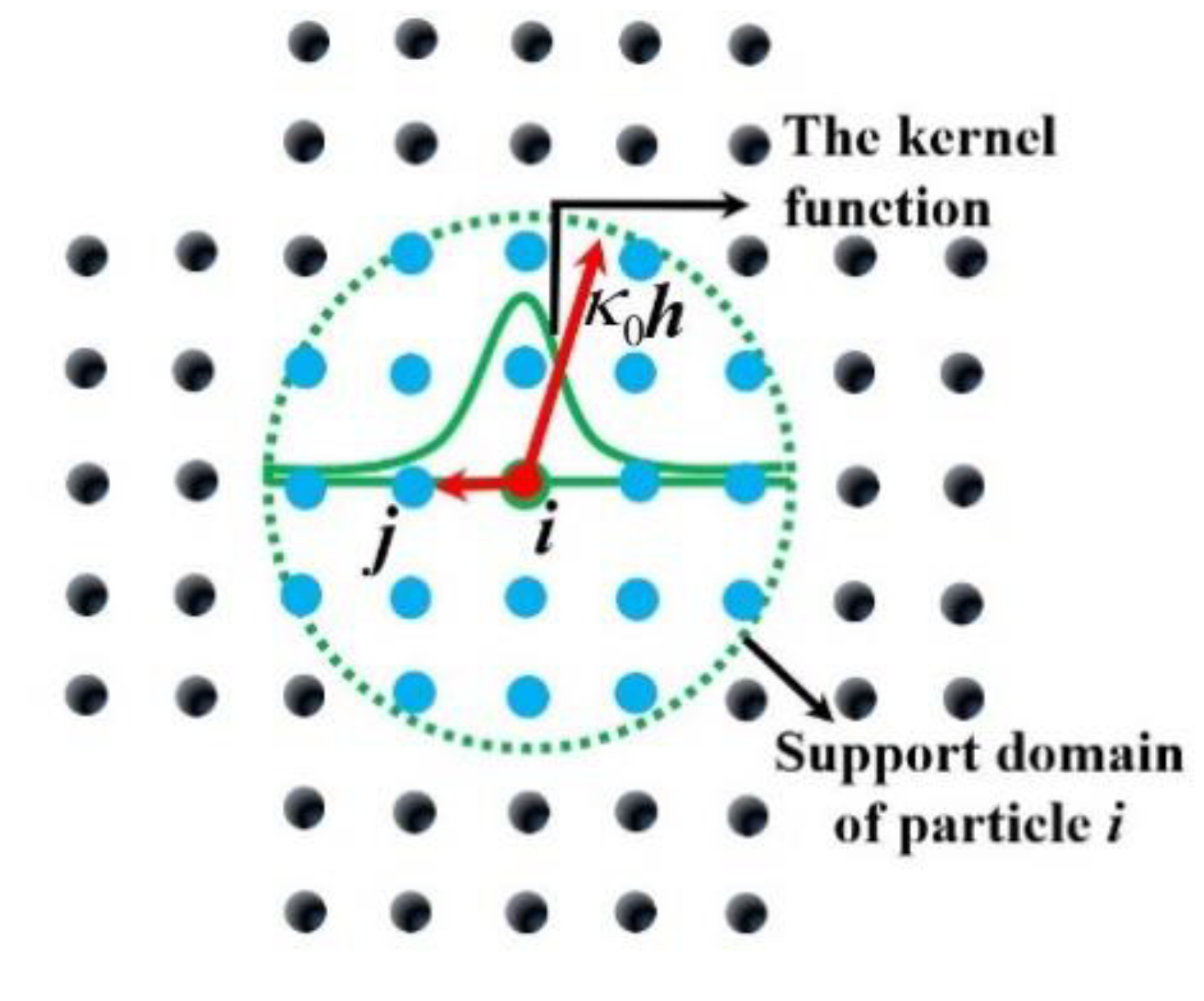
2.1. Smoothed Particle Hydrodynamics

The Lagrangian form of the conservation laws for the continuity and momentum describing the flow of a weakly compressible flow can be written as

$$\frac{D\rho }{Dt}=-\rho \nabla \cdot u,$$

(1a)

$$\frac{Du}{Dt}=\frac{1}{\rho }\nabla \cdot \sigma +f,$$

(1b)

where u and ρ are the total velocity and the density field of the fluid, respectively, f is an acceleration resulting from an external force, σ is the stress tensor consisting of pressure gradient and viscous terms. In the framework of SPH, the discretized form of the continuity equation, i.e., Equation (1a) is written as

$${\left\{\frac{D\rho }{Dt}\right\}}_i={\rho }_i{\displaystyle \sum _j\frac{m_j}{{\rho }_j}}{u}_{ij}\cdot {\nabla }_i{W}_{ij}+{\delta }_i,$$

(2a)

where W is the smoothing kernel function, for which the cubic spline kernel outlined in Monaghan and Lattanzio [22] is used in this study. Figure 1 shows a schematic of an SPH particle in its support domain wherein the physical quantities of particle i are obtained by interpolating the quantities of the particles in its support domain using the kernel function. The kernel function has a compact support domain Ω which is a circle of radius κ₀h, where κ₀ is a parameter varying with the chosen kernel function shown in Figure 1, and it is equal to two for cubic spline kernel. The smoothing length h = δ_sR is related to the support area over which approximations are estimated, R is the resolution, i.e., initial interparticle gap, and δ_s is the smoothing factor, the value of which is typically in the range of 1.25~2 depending on the specific flow being considered. For WSI problems, convergent results are usually obtained by choosing the smoothing factor as 1.5, which has been used for most of the problems reported in this study, unless specified otherwise. The additional term δ_i is introduced to improve the stability of the SPH numerical calculation [23] and to remove spurious pressure oscillations that can exist in weakly compressible SPH. The vector u_ij denotes the difference between u_i and u_j at locations i and j, as indicated in Figure 1.

The discretized form of the momentum conservation equation, i.e., Equation (1b), for the single- and two-phase flows considered in this study takes the following form as shown in [24]

$${\left\{\frac{Du}{Dt}\right\}}_i=-\frac{1}{m_i}{\displaystyle \sum _j\left(P_i{(\frac{m_i}{{\rho }_i})}^2+P_j{(\frac{m_j}{{\rho }_j})}^2+{\mathrm{\Pi }}_{ij}\right)}\cdot {\nabla }_i{W}_{ij}+{\displaystyle \sum _j{m}_j}\left(\frac{2\mu r_{ij}\cdot {\nabla }_i{W}_{ij}}{{\rho }_i{\rho }_j{\left|r\right|}_{ij}}{u}_{ij}\right)+g$$

(2b)

where P_i and P_j are the pressures at particle i and particle j, respectively, r_ij is the displacement vector from particle i to particle j, g is the gravitational acceleration and μ is the dynamic viscosity of the fluid which is assumed to be constant in this study. The term Π_ij denotes the artificial viscosity introduced to alleviate pressure oscillations caused by a non-physical concentration of particles and is modeled as in [25]

$${\prod }_{ij}^{}=\frac{-\alpha \overline{c_{ij}}{\varphi }_{ij}}{\overline{{\rho }_{ij}}} \mathrm{if} u_{ij}{r}_{ij}<0 \mathrm{and} {\prod }_{ij}^{}=0 \mathrm{if} u_{ij}{r}_{ij}\ge 0,$$

(2c)

where ${\varphi }_{ij}^{}=\frac{h{u}_{ij}{r}_{ij}}{{\left|r_{ij}\right|}^2+{\eta }^2}$, $\overline{{\rho }_{ij}}$ and $\overline{c_{ij}}$ are respectively the average values of the density and the sound speed of particle i and j. η = 0.1 h is chosen to prevent the numerical divergence when particles are close to each other, α is a parameter which is set according to the flow problem with the guidance that a proper value of α should not be too large as it may lead to a large error, and should not be too small to avoid being ineffective in alleviating the oscillations in dynamic problems. For all the WSI problems considered in this study, the value of α is in the range 0.01~0.05. For the weakly compressible flow, an equation of state which is commonly used in SPH to relate the pressure to small variations of fluid density is applied

$$P=B\left({\left(\frac{\rho }{{\rho }_0}\right)}^{{\gamma }_0}-1\right),$$

(3)

where B is the reference pressure defined as $B=\frac{{\rho }_0{c}^2}{{\gamma }_0},$ ${\rho }_0$ is the fluid reference density (for the water and air, they are, respectively, 1000 kg/m³ and 1.29 kg/m³), c is the speed of sound in the fluid, ${\gamma }_0$ is a constant, and a value ${\gamma }_0=7$ is used for the problems in this study. A proper value of B is chosen to ensure that the compressibility effects are negligible [26], and for this, the speed of sound should satisfy c ≥ 10 max(||u_max||). The general form of Equations (2a) and (2b) can be written as

$${\left\{\frac{DU}{Dt}\right\}}_i=S_i$$

(4)

$$\mathrm{where} U={\left[\begin{array}{c}\rho \\ u\end{array}\right]}_i\mathrm{and} S_i=\left[\begin{array}{c}{\rho }_i{\displaystyle \sum _j\frac{m_j}{{\rho }_j}}{u}_{ij}\cdot {\nabla }_i{W}_{ij}+{\delta }_i\\ -\frac{1}{m_i}{\displaystyle \sum _j\left(P_i{(\frac{m_i}{{\rho }_i})}^2+P_j{(\frac{m_j}{{\rho }_j})}^2+{\mathrm{\Pi }}_{ij}\right)}\cdot {\nabla }_i{W}_{ij}+{\displaystyle \sum _j{m}_j}\left(\frac{2\mu r_{ij}\cdot {\nabla }_i{W}_{ij}}{{\rho }_i{\rho }_j{\left|r\right|}_{ij}}{u}_{ij}\right)+g\end{array}\right] .$$

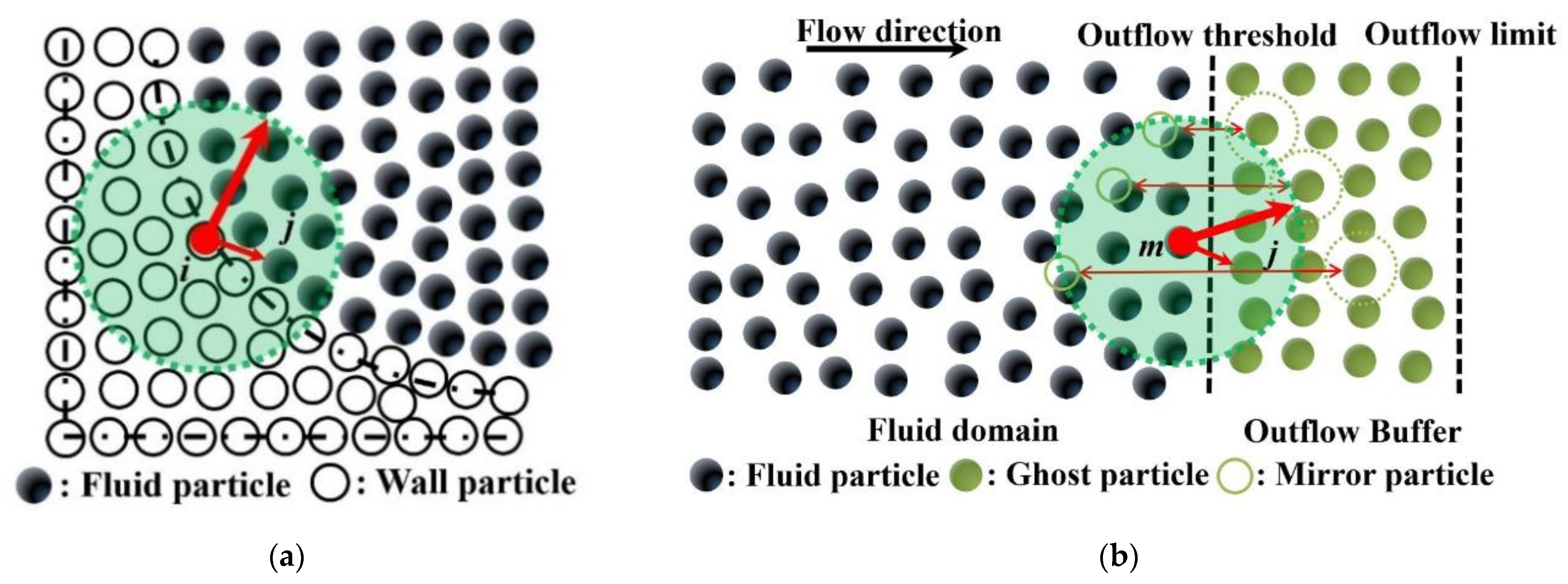
2.2. Boundary Conditions

For the problems of interest, both wall boundary and open boundary conditions are considered. The no-slip boundary conditions are imposed at solid walls as specified in [27]. As shown in Figure 2a, the pressure on the solid particle i is extrapolated from the neighboring fluid particle j,

$$P_i=\frac{{\displaystyle \sum _j\left(P_j+\left(g_j\cdot r_{ij}\right){\rho }_j\right)W_{ij}}}{{\displaystyle \sum _j{W}_{ij}}}.$$

(5)

The corresponding densities are then estimated using Equation (3).

Open boundary conditions are usually implemented at the inflow or the outflow boundaries of the flow domain of interest by imposing zero velocity or zero pressure gradients. Recently, a versatile open boundary condition for SPH simulation outlined in [28] incorporates a buffer layer consisting of ghost particles, the width of which usually corresponds to the support domain radius. Figure 2b shows a schematic of the implementation of open boundary conditions at the outflow boundary, indicating the mirror particles mirrored from ghost particles relative to the outflow threshold for facilitating density and velocity interpolations. The new incoming particles will be added layer by layer with a uniform interval (initial interparticle gap), and the outgoing particles will be deleted. At the inflow boundaries, the velocity of the ghost particles is prescribed based on the flow problem, and the density is interpolated from the fluid or ghost particles. Both the ghost particles’ velocity and density are interpolated from the fluid or ghost particles at the outflow boundaries.

The physical quantities of the mirrored particles are then projected back to the corresponding ghost particles using the first-order Taylor series expansion. The interpolation schemes used for estimating the approximate values of the physical quantities R_m and their first-order derivatives R_m,β ensures the consistency of the kernel function as pointed out in [29], and takes the form

$$R_m=\frac{\left|\begin{array}{l}{\displaystyle \sum _j{R}_j{V}_j{W}_{mj} {\displaystyle \sum _j\left(x_j^{\beta }-x_m^{\beta }\right)V_j{W}_{mj}}}\\ {\displaystyle \sum _j{R}_j{V}_j{W}_{mj,\gamma } {\displaystyle \sum _j\left(x_j^{\beta }-x_m^{\beta }\right)V_j{W}_{mj,\gamma }}}\end{array}\right|}{\left|\begin{array}{l}{\displaystyle \sum _j{V}_j{W}_{mj} {\displaystyle \sum _j\left(x_j^{\beta }-x_m^{\beta }\right)V_j{W}_{mj}}}\\ {\displaystyle \sum _j{V}_j{W}_{mj,\gamma } {\displaystyle \sum _j\left(x_j^{\beta }-x_m^{\beta }\right)V_j{W}_{mj,\gamma }}}\end{array}\right|} ,R_{m,\beta }=\frac{\left|\begin{array}{l}{\displaystyle \sum _j{V}_j{W}_{mj} {\displaystyle \sum _j{R}_j{V}_j{W}_{mj}}}\\ {\displaystyle \sum _j{V}_j{W}_{mj,\gamma } {\displaystyle \sum _j{R}_j{V}_j{W}_{mj,\gamma }}}\end{array}\right|}{\left|\begin{array}{l}{\displaystyle \sum _j{V}_j{W}_{mj} {\displaystyle \sum _j\left(x_j^{\beta }-x_m^{\beta }\right)V_j{W}_{mj}}}\\ {\displaystyle \sum _j{V}_j{W}_{mj,\gamma } {\displaystyle \sum _j\left(x_j^{\beta }-x_m^{\beta }\right)V_j{W}_{mj,\gamma }}}\end{array}\right|,}$$

(6)

where the index m denotes the mirror particles, and j represents the fluid or ghost particle inside the support domain of particle m, β and γ are the indices of dimensions repeated from one to two or three, and W_mj,γ = ∂W_mj/∂x^γ (∂x^γ means ∂x, ∂y or ∂z) are the spatial derivatives of the kernel function for which a first-order Taylor series expansion around the location of particle m can be written as

$$R_{n_0}=R_m+\left(x_{n_0}^{\beta }-x_m^{\beta }\right)R_{m,\beta },$$

(7)

where n₀ denotes the ghost particle corresponding to the mirror particle m.

2.3. Time Integration Schemes

A velocity-Verlet [30] scheme, a special form of the Newark-beta method for integrating differential equations as outlined in [31] was used for the time integration. Note that for the two-phase flows, the continuity and momentum equations of the air phase and water phase are calculated simultaneously (Equations (1a) and (1b)), hence the “fluid” is used to denote both the air and water in the time integration process. The velocity and displacement of the fluid particles are updated at the end of the first half of each time step

$$u^{n+\frac{1}{2}}=u^n+\frac{D{u}^n}{Dt}\frac{\Delta t}{2},$$

(8a)

$$r^{n+\frac{1}{2}}=r^n+u^{n+\frac{1}{2}}\frac{\Delta t}{2}.$$

(8b)

where the superscript n denotes the time step. Then the continuity Equation (2a) is integrated using the updated velocity Equation (8a) to update the density and the displacement Equation (8b) of the fluid particles over the next half of the time step so that at the end of each time step

$${\rho }^{n+1}={\rho }^n+\frac{D{\rho }^{n+\frac{1}{2}}}{Dt}\Delta \mathrm{t},$$

(8c)

$$r^{n+1}=r^{n+\frac{1}{2}}+u^{n+\frac{1}{2}}\frac{\Delta t}{2}.$$

(8d)

For a floating structure governed by the rigid body motion equations, its velocity and displacement are updated after the total force F and total moment T acting on the solid body are obtained

$$\frac{D{U}^{n+\frac{1}{2}}}{Dt}=F\left(P\left({\rho }^{n+1}\right),\Pi \left(u^{n+\frac{1}{2}}\right),g\right),$$

(8e)

$$\frac{D{\Omega }^{n+\frac{1}{2}}}{Dt}=T\left(P\left({\rho }^{n+1}\right),\Pi \left(u^{n+\frac{1}{2}}\right),X_0\right),$$

(8f)

$$U^{n+1}=U^n+\frac{D{U}^{n+\frac{1}{2}}}{Dt}\Delta \mathrm{t},$$

(8g)

$${\Omega }^{n+1}={\Omega }^n+\frac{D{T}^{n+\frac{1}{2}}}{Dt}\Delta \mathrm{t},$$

(8h)

$$r_s{}^{n+1}=r_s{}^n+\left(U^{n+1}+{\Omega }^{n+1}\times \left(r_s^n-X_0\right)\right)\Delta \mathrm{t},$$

(8i)

where X₀, U, Ω, and r_s are, respectively, the mass center location, the translation velocity, the rotation velocity, and the solid particle location of the structure. In Equations (8e) and (8f), the functions are used for the convenience of expressing the suffered total force and moment of a floating structure. The forces on the boundary particle i of the floating structure exerted by the neighboring fluid particle j are based on Equation (2b)

$$f_i^{\mathrm{s}}=m_i\left[-\frac{1}{m_i}{\displaystyle \sum _j\left(P_i{(\frac{m_i}{{\rho }_i})}^2+P_j{(\frac{m_j}{{\rho }_j})}^2+{\Pi }_{ij}\right)}\cdot {\nabla }_i{W}_{ij}+{\displaystyle \sum _j{m}_j}\left(\frac{2\mu r_{ij}\cdot {\nabla }_i{W}_{ij}}{{\rho }_i{\rho }_j{\left|r\right|}_{ij}}{u}_{ij}\right)+g\right].$$

(8j)

Hence the details of Equations (8e) and (8f) are expressed as

$$M\frac{DU}{Dt}={\displaystyle \sum _i{f}_{\mathrm{i}}^{\mathrm{s}}}+Mg,$$

(8k)

$$I\frac{D{\Omega }^{n+\frac{1}{2}}}{Dt}={\displaystyle \sum _i\left(r_{\mathrm{s}}-X_0\right)}\times f_{\mathrm{i}}^{\mathrm{s}},$$

(8l)

where M and I are, respectively, the mass and the moment of inertia of the floating structure. Note that for the case of two freely floating boxes with collision, an elastic collision force which will be addressed later in this section, should be added in Equations (8k) and (8l), respectively. Subsequently, the velocity of the fluid particles is updated at each half time step,

$$u^{n+1}=u^{n+\frac{1}{2}}+\frac{D{u}^{n+1}}{Dt}\frac{\Delta t}{2}.$$

(8m)

Using the velocity computed at the end of the half-time step, the force is computed only once per time step to obtain the particle acceleration after the density is updated to Equation (8c). To obtain a proper time step, several criteria outlined in [25] must be satisfied for the stability reasons of the numerical scheme. Namely, the CFL-condition related to the smoothing length h, the maximum sound speed c_max (c_max must be estimated according to the specific flow problems before calculating, and the actual value may be smaller for obtaining better numerical results), the maximum flow speed u_max, the viscosity v as well as the body force g, are adopted to estimate the global time step. It requires,

$$\Delta \mathrm{t}\le 0.25\frac{h}{c_{\max }+‖u_{\max }‖},$$

(9a)

$$\Delta \mathrm{t}\le 1.25\frac{h^2}{v},$$

(9b)

$$\Delta \mathrm{t}\le 0.25{\left(\frac{h}{‖g‖}\right)}^{\frac{1}{2}}.$$

(9c)

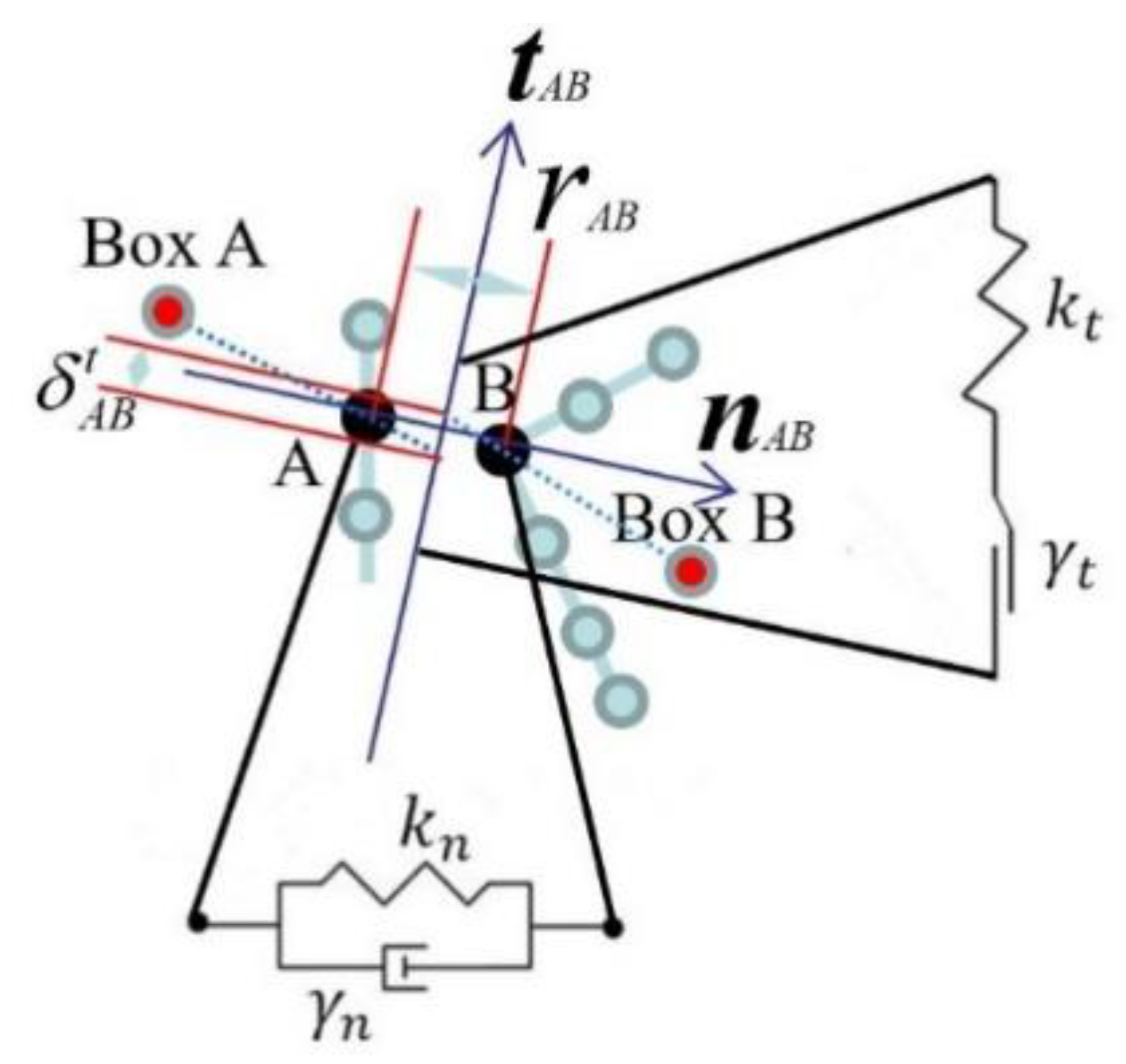
2.4. Collision Force Model

When the two boxes are very close to each other, a collision occurs and this is modeled based on the discrete element method (DEM) [32]. As indicated in Figure 3, the contact force F_c acting on box A resulting from a collision with Box B can be decomposed into the normal and tangential components F_n and F_t, respectively. Both the forces can be further decomposed into a repulsion force F^r and a damping force F^d, which are respectively caused by the deformation of the material and the dissipation of energy during the deformation. The normal forces can be expressed as [33]

$$F_{n,AB}=F_n^r+F_n^d=k_{n,AB}{\delta }_{AB}^{3/2}{e}_{AB}-{\gamma }_{n,AB}{\delta }_{AB}^{1/4}{\dot{\delta }}_{AB}{e}_{AB},$$

(10a)

where k_n,AB is the stiffness constant of the boxes; δ_AB = R-r_AB is the box overlap (see Figure 3, R is the initial interparticle gap or the resolution); e_AB is the unit vector between particles of the two boxes with the minimum distance (see Figure 3, the distance between point A and point B); ${\dot{\delta }}_{AB}=v_{AB}\cdot e_{AB}$ is the rate of normal deformation (see Figure 3, v_AB is the velocity difference between point A and point B); ${\gamma }_{n,AB}$ is the damping constant. The stillness and damping constants are, $k_{n,AB}$=$\frac{4}{3}{E}^{*}\sqrt{R^{*}}$ and ${\gamma }_{n,AB}$=$C_n\sqrt{6M^{*}{E}^{*}\sqrt{R^{*}}}$, respectively, where C_n is in order of 10⁻⁵ [34]; E* = $\frac{E_b}{1-{\nu }_b^2}$ (E_b is the Young modulus, v_b is the Poisson ratio); R* and M* are, respectively, half of the height and mass of the boxes. The tangential forces are given similarly to [35]

$$F_{t,AB}=\min ({\mu }_{f,AB}{F}_{n,AB}^{}\tanh (8{\dot{\delta }}_{AB}^t)e_{AB}^t;\hspace{0.33em}{F}_t^r+F_t^d),$$

(10b)

where $F_t^r+F_t^d=k_{t,AB}{\delta }_{AB}^t{e}_{AB}^t-{\gamma }_{n,AB}{\dot{\delta }}_{AB}^t{e}_{AB}^t$ with $k_{t,AB}=\frac{2}{7}{k}_{n,AB}$ and ${\gamma }_{t,AB}=\frac{2}{7}{\gamma }_{n,AB}$; the superscript or subscript t denotes the tangential direction; μ_f,AB is the kinetic friction coefficient. In the present study, the boxes are assumed to be made of hardwood, corresponding to Young modulus E_b = 2 × 10⁸ N/m², Poisson ratio v_b = 0.2, and the kinetic friction coefficient μ_f,AB = 0.7.

3. Numerical Results and Discussion

In this section, the SPH simulations of several two-phase WSI examples are discussed. First, a classical two-phase dam-breaking problem is addressed to show the convergence issues of the SPH method. Next, a two-phase SPH simulation of a second-order wave generated by a piston in a wave basin is validated to capture the wavy air-water interface. This is followed by the two-phase SPH simulation of the interaction between the wave generated in the wave basin and a rigid cantilever beam fixed to the bottom of the wave basin and downstream of the wavemaker mechanism. Subsequently, the two-phase SPH simulation of the interaction between the wave and a floating box to capture the wave-induced motion of the box is conducted. The two-phase SPH simulation of the interaction between the wave and two identical floating boxes with the possibility of elastic collision between them is considered finally.

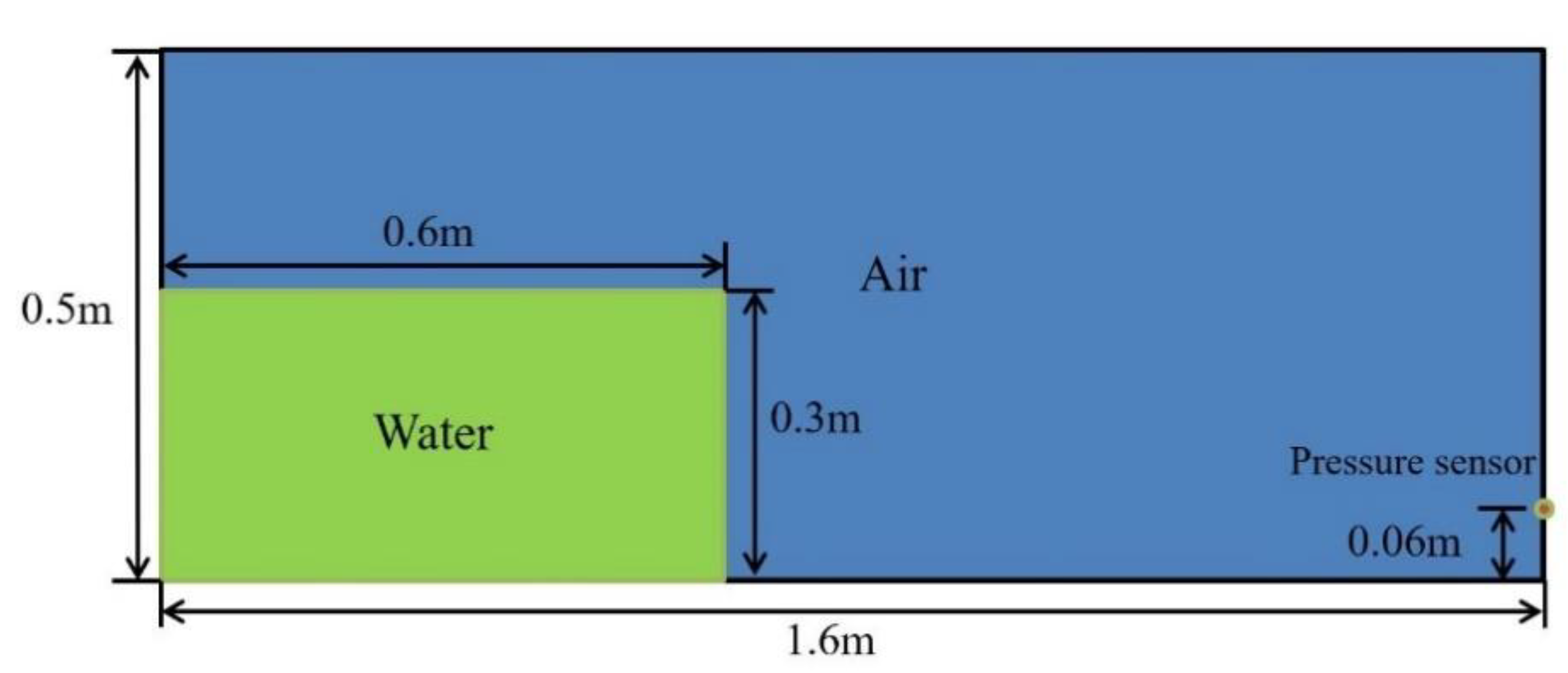
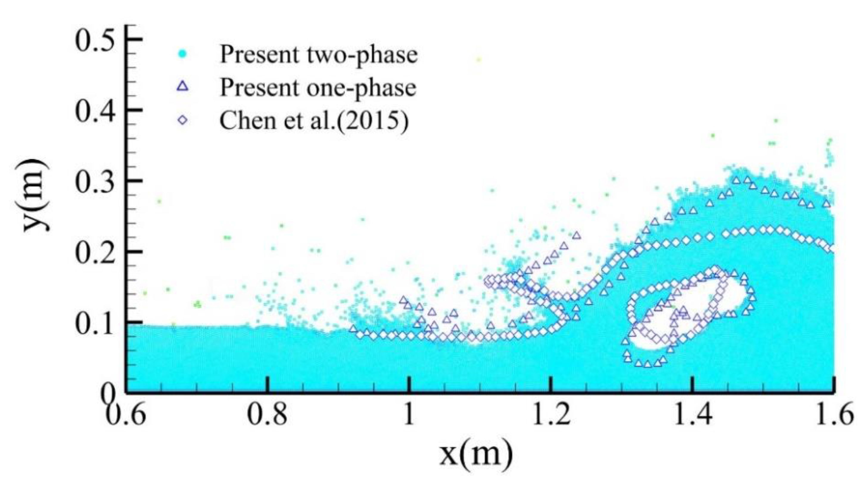
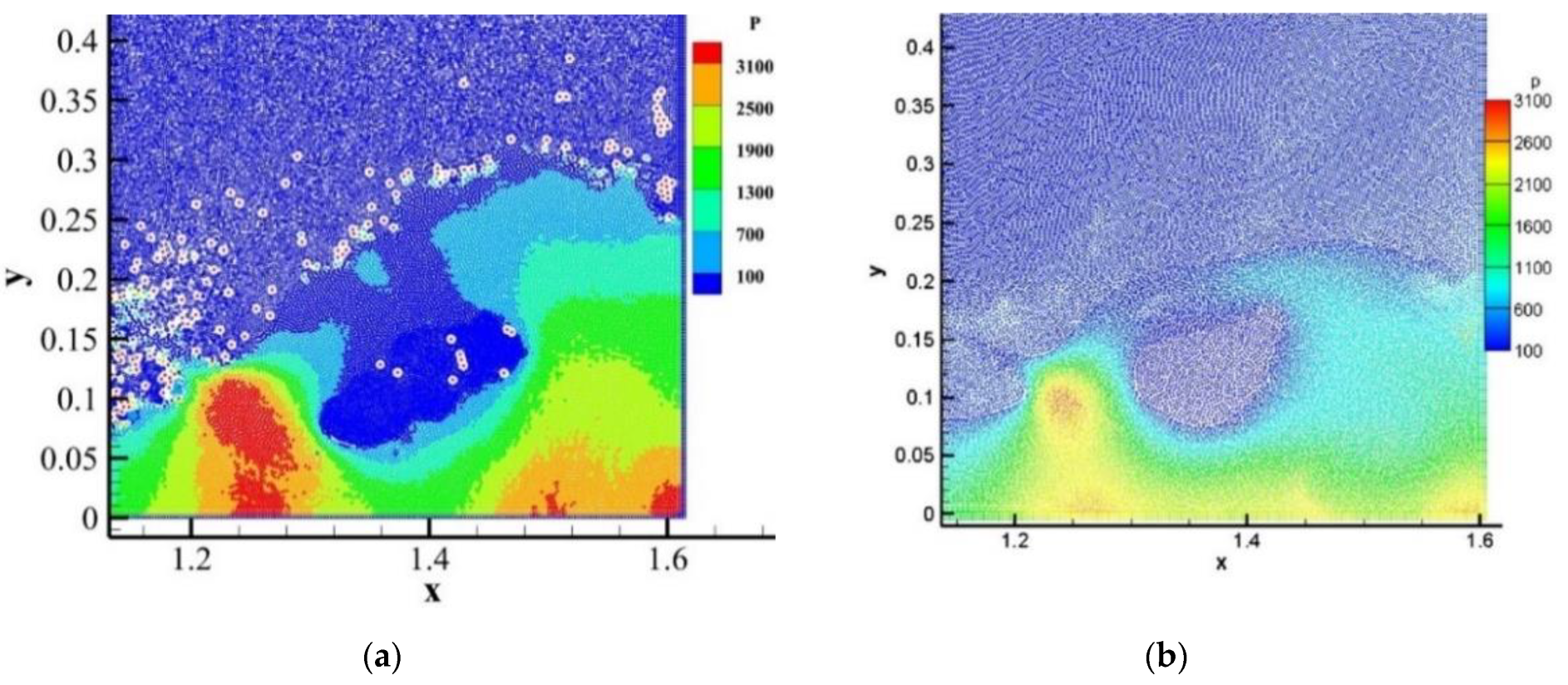
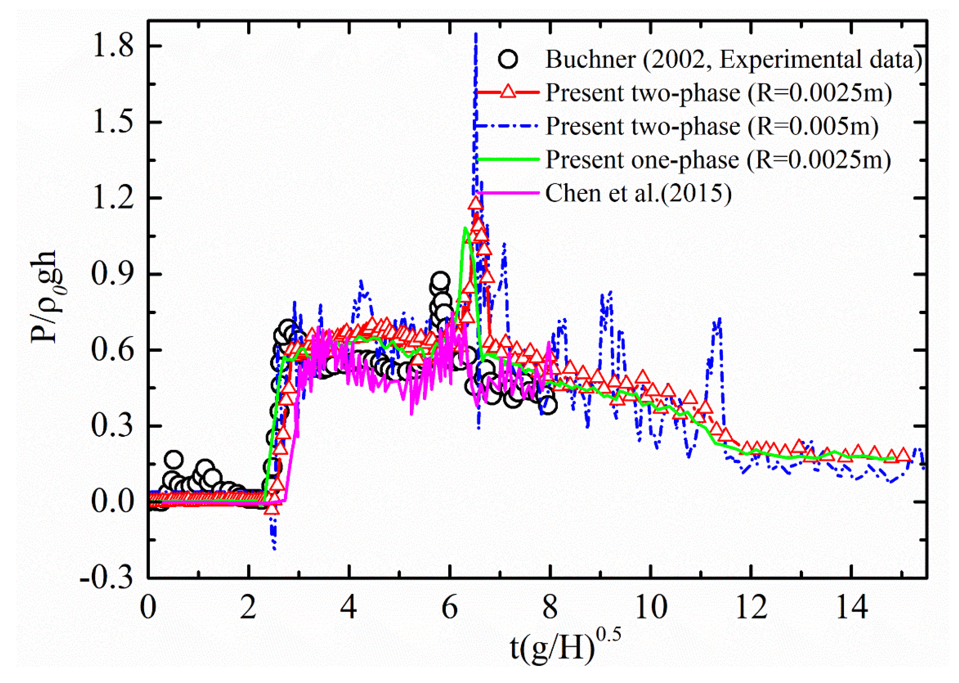
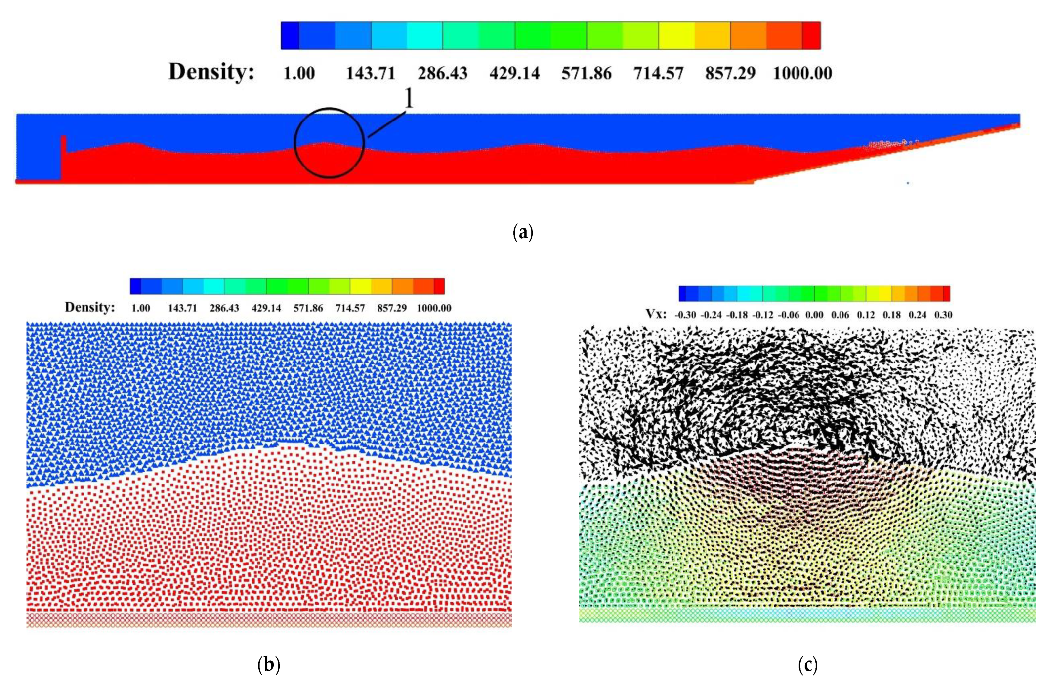
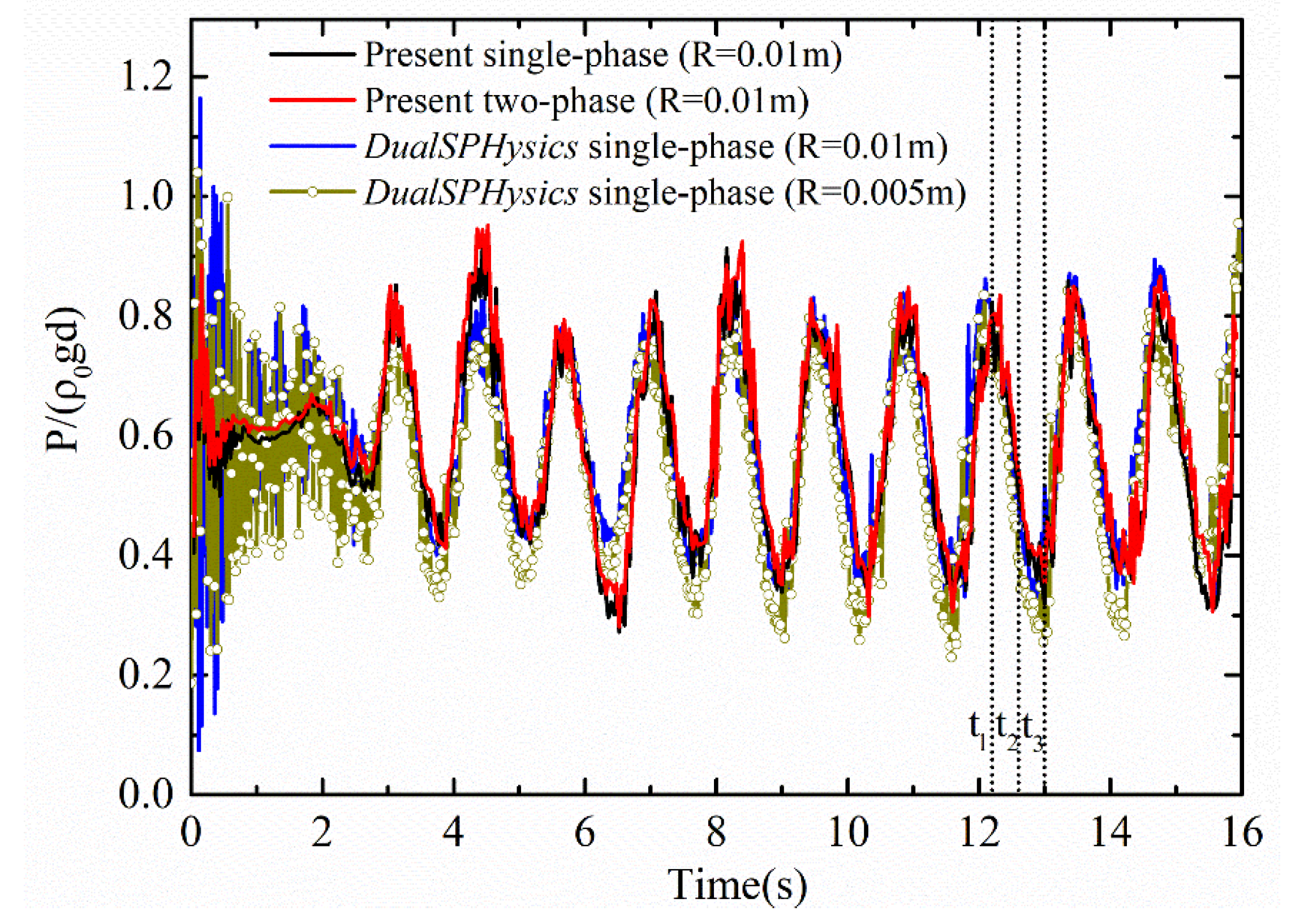
3.1. SPH Simulation of Dam-Breaking

The two-phase dam-breaking problem is a standard benchmark test case that has several hydrodynamic phenomena such as a surface break-up, water jet, and impact pressure. This test was chosen for validating the accuracy and stability of the present two-phase SPH code given the large difference in the densities of the two phases, namely air and water. The computational domain is shown in Figure 4, the height and length of the computational domain are, respectively, 0.5 m and 1.6 m. The water is initially contained in a rectangular domain (dam) with a length L of 0.6 m and a height H of 0.3 m (shaded in light green) implying a volume of water per unit width of 0.18 m³. The remaining area of the computational domain (shaded in light blue) is assumed to be filled with air. Both air and water are assumed to be at rest initially and t = 0 is defined as the instant at which the water dam is allowed to break free and fall. The no-slip condition is imposed on the solid walls. The total number of particles N used for this computation is 158916 (5316 for solid walls, 34560 for water, and 119040 for air). A smoothing length h = 1.5 R with a resolution R = 0.0025 m is used. Following the work of Gong et al. [36], the laminar viscosity is ignored. The artificial viscosity term α of 0.05 and a fixed computational time step of 5 × 10⁻⁵ s have been used for this problem. The evolution of the solution in the computational domain is then tracked in terms of a non-dimensional time step $\overline{t}$ defined as t(g/H)^0.5. Note that the theory of the two- and single-phase simulation is integrated into Equation (4), hence we only need to remove the air particles when considering the single-phase flow problem.

Figure 5 compares the contours of the computed water heights in the computational domain at $\overline{t}$ = 0.64 after the dam-breaking. The computed water heights from both single- and two-phase SPH simulations are compared with the two-phase result of Chen et al. [37] at the same instant. It can be seen that after impacting the vertical wall w the pressure sensor is located (see Figure 4), the water height reaches a relatively higher level than that predicted by a single-phase SPH and also with that predicted in [37]. An area of air entrapment can also be seen here. Apart from the area of the air bubble entrapped by the backward plunging breaker, it can be seen that the outline of the water height from the single-phase flow is comparable with that from the two-phase flow. It is observed that the two-phase SPH simulation forms a smoother interface of entrapped air due to the weak compressibility of the air phase there.

Figure 6 compares the computed spatial pressure contours from the present two-phase SPH model with that from reference [37] at the same instant, and while there are differences in the contour levels, the spatial distribution is similar. This is due to the different wall boundary conditions, in which a comparatively higher pressure is obtained in our simulations (see Figure 7). Note that the air and the water are presented in Figure 6. The splashed water particles (see Figure 6a) with uneven distribution may be affected by the higher pressure (compared to that of the reference [37]). Note that the pressure below the cavity is comparatively larger than that acting on the cavity top. This pressure difference leads to the collapse of the cavity for the single-phase flow without the air (see Figure 5 and Figure 6a).

Figure 7 compares the temporal variation of the pressure recorded at the pressure sensor placed on the wall at a height of 0.06 m from the base, as shown in Figure 4, corresponding to single- and two-phase SPH simulations from the present study and also with that from Chen et al. [37] and Buchner [38]. For the two-phase SPH simulations, two resolutions have been considered, i.e., R = 0.005 m and 0.0025 m, to gauge the convergence of the pressure temporal variation. It can be seen that the choice of the resolution of 0.0025 results in a smoothening of the pressure variation and improves the predicted temporal pressure evolution agreement with that of Chen et al. [37]. Compared to Buchner’s experimental data [38], it appears that the present SPH models give a reliable prediction of the pressure evolution. The pressure of the two-phase simulation lags a little from the single-phase result in time scale, which is due to the compression of the surrounding air. The simulation results also lag from the experimental data, which may be due to the present SPH’s weakly compressibility. The pressure peak of the sensor in our simulation appears at $\overline{t}$ = 6.4 when the backward plunging breaker entraps the air and creates the cavity (see Figure 5 and Figure 6). Subsequently, it gradually reaches the expected hydrostatic pressure.

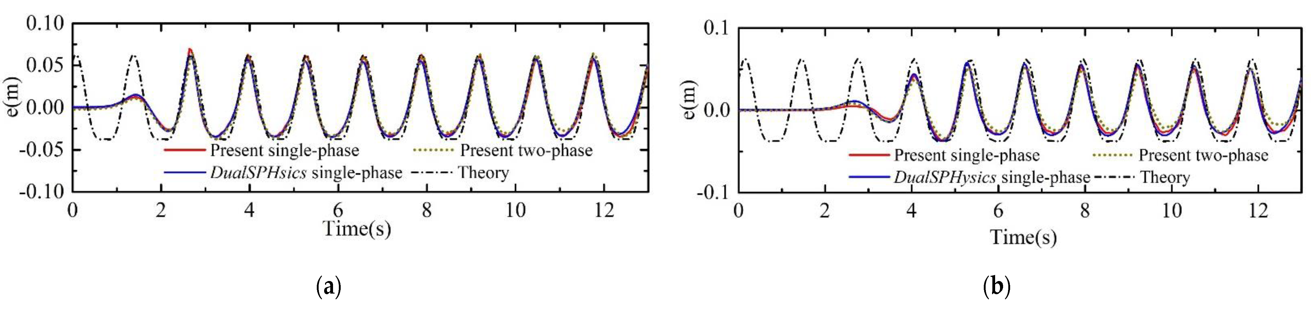
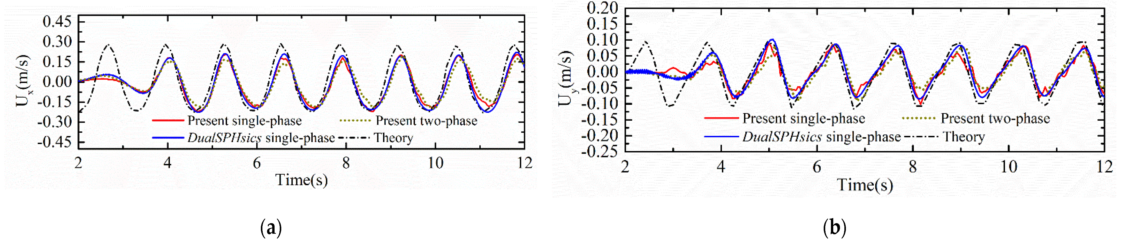
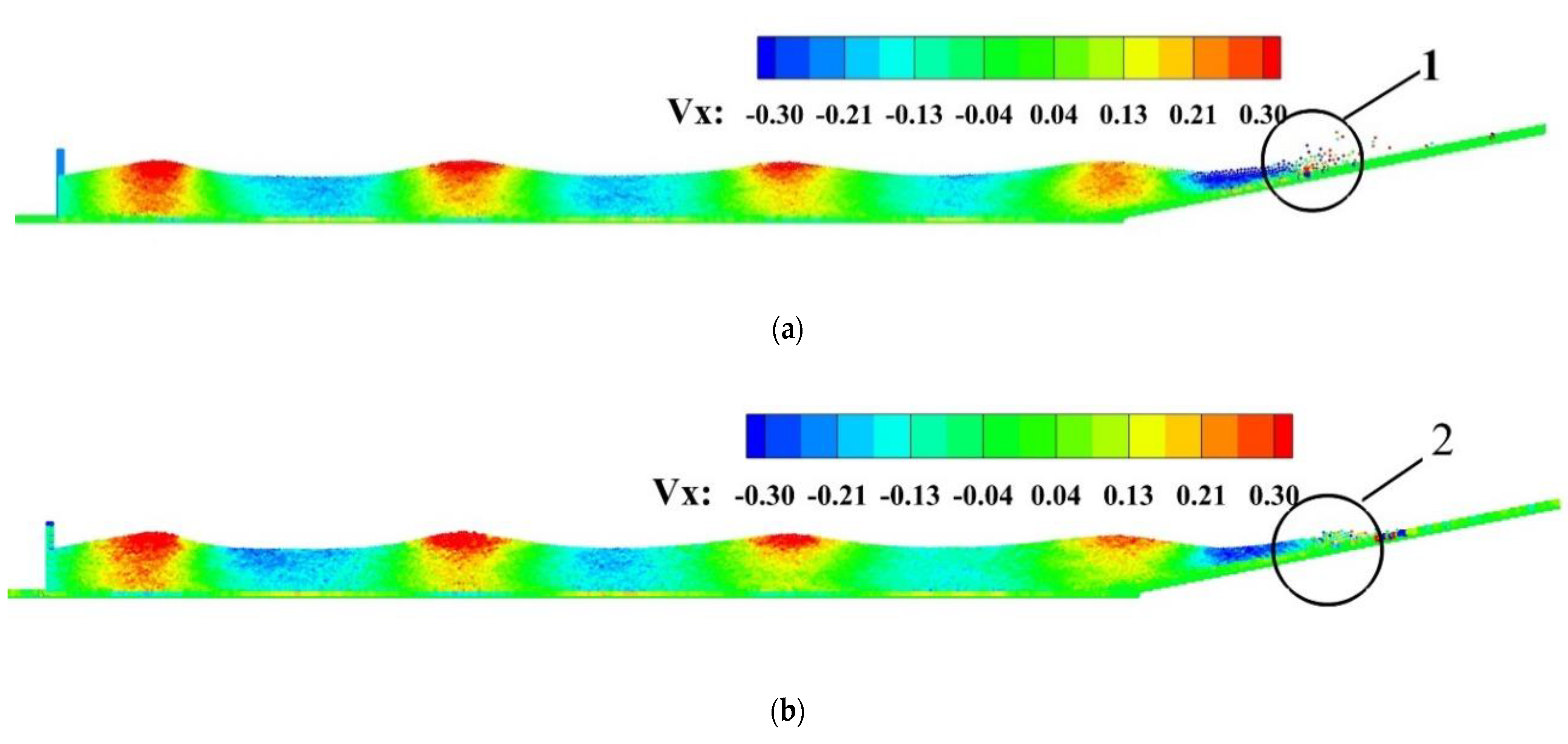
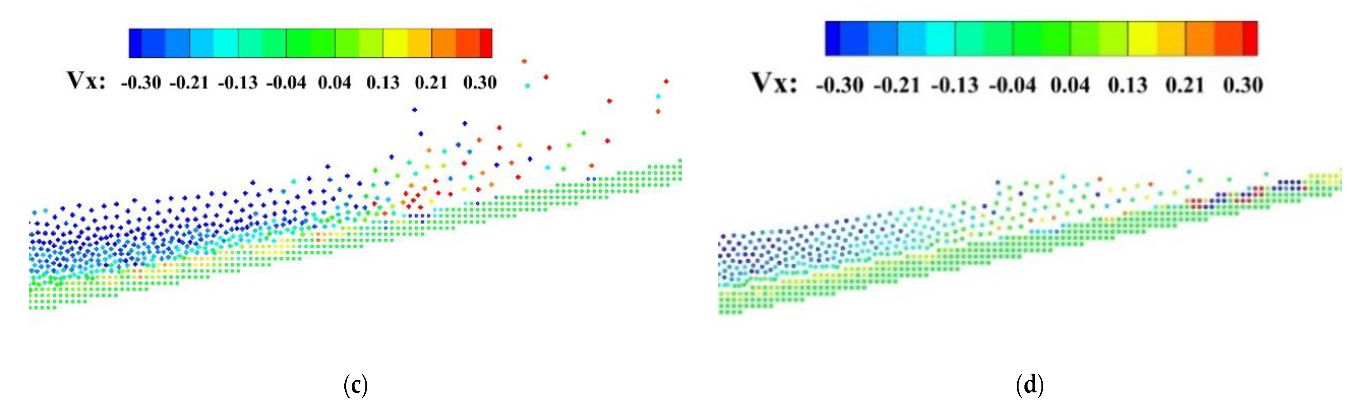
3.2. Two-Phase Wave Generation in a Wave Basin

This section is concerned with the generation of waves in a two-phase flow in a wave basin. Based on the assumptions of irrotational and incompressible fluid and constant pressure at the free surface, the Biesel transfer function outlined in [39] and also in [40] can be used to describe the relation between wave amplitude and wavemaker displacement. The far-field solution for the free-surface elevation is expressed as

$${\eta }_0\left(x,t\right)=\frac{H_0}{2}\cos \left(\omega t-kx+{\delta }_0\right),$$

(11)

where H₀ is the wave height, ω = 2π/T is the angular frequency, k = 2π/𝜆 is the wavenumber, T is the wave period, 𝜆 is the wavelength and the initial phase δ₀ is given by a random number between 0 and 2π. For a piston-type wavemaker, the Biesel transfer function under the hypothesis of monochromatic sinusoidal waves is expressed as

$$\frac{H_0}{S_0}=\frac{2{\sinh }^2\left(kd\right)}{\sinh \left(kd\right)\cosh \left(kd\right)+kd},$$

(12)

where S₀ is the piston stroke and d is the water depth. The time series of the piston motion is then given by

$$e\left(t\right)=\frac{S_0}{2}\sin \left(\omega t+{\delta }_0\right).$$

(13)

Madsen [41] has developed a simple second-order wavemaker theory to generate relatively long second-order Stokes waves that preserve shape as they propagate. To generate second-order regular waves, an additional term is added to Equation (13) to account for the piston displacement so that

$$e\left(t\right)=\frac{S_0}{2}\sin \left(\omega t+{\delta }_0\right)+\left[\left(\frac{H_0{}^2}{32d}\right)\left(\frac{3\cosh \left(kd\right)}{{\sinh }^3\left(kd\right)}-\frac{2S_0}{H_0}\right)\right]\sin \left(2\omega t+2{\delta }_0\right).$$

(14)

In the present study, the second-order Stokes waves are generated using a piston-type wavemaker as shown in Figure 8, which shows the wave basin configuration and the computational domain for the two-dimensional two-phase wave basin. In the following content, based on the above wave making theory, we first generate the second-order Stokes wave using the SPH method, and then validate our results against the theoretical solution. The selection of the wave parameters is based on the existing literature research and the specific problems we face in our project. This step is to lay the foundation for the later study of the interaction between the waves and fixed structures, and between the waves and the freely floating boxes.

The open boundary conditions are implemented at Buffer 1 and Buffer 2 (indicated in green patches) with the initial density set to the air density, and the dimensions of the air phase space are set to a height of d_a = 0.35 m from Buffer 2 and a width S_a of 0.4 m. Note that Buffer 1 and Buffer 2 only refer to the air phase. Hence, the open boundary condition aforementioned for a single-phase problem in Section 2.2 is effective to handle this case. Regular water waves are propagated along the 6-m-long basin with the distance parameter a indicated in Figure 8 defined as 1 m. The basin has a 1:5-sloped beach at the end to absorb the waves. The no-slip boundary conditions are implemented at the bottom wall and the dissipative beach. Wave gauges WG1, WG2, and WG3, are the locations where the sensors are set to monitor the wave velocity and the height from the basin bottom. The initial water depth d, wave height H₀, period T, and wavelength λ are assigned values of 0.27 m, 0.1 m, 1.3 s, and 1.89 m, respectively. For this computation, a smoothing length h of 1.5 R and a resolution of R = 0.01 m correspond to 3216 particles for the wall, 21900 particles for single-phase SPH, and 53161 particles (31261 particles for the air and 28584 particles for the water) for the two-phase SPH simulations. The artificial viscosity parameter α in Equation (2b) and the computational time step are set to 0.01 and 1 × 10⁻⁴ s, respectively. Note that in this case, the cantilever beam does not exist.

Figure 9 compares the computed temporal variation of the free surface wave elevations recorded at the wave gauges WG1 and WG3 placed at x = 2 m and 4 m, respectively. It is observed that the results from the present single-phase and two-phase SPH and DualSPHysics match the theoretical solution to a good extent, although the wave troughs are slightly overestimated (less than 3%) by SPH, indicating that the waves are properly generated, and the effect of the air on the wave elevations appears to be negligible. Note that the results of DualSPHysics are obtained by us, rather than from the literature. Figure 10 compares the computed velocity components from theory and DualSPHysics corresponding to the same case shown in Figure 9. The horizontal and vertical velocity components are monitored at a height d₂ of 0.12 m above the basin in the WG3 profile. Apart from the horizontal velocity, which is slightly underestimated at the peak, the results could provide a satisfactory accuracy.

Figure 11a,b shows the contours of the horizontal velocity contours for single-phase and two-phase wave generation at the instant t = 16 s, respectively. In Figure 11b, the air particles are not shown deliberately to understand the physics predicted by the single- and two-phase SPH. It can be observed that the same velocity patterns and free-surface profiles are predicted by the two approaches from a global viewpoint. However, if one focuses on the circled regions in the vicinity of the sloped dissipative beach area labeled and shown in Figure 11c,d, respectively, it is observed that the water particles of the single-phase simulation splash more severely than those of the two-phase simulation. This indicates that air in the vicinity could smoothen the air-water interface by complementing the particles for the calculation in the vicinity of the water surface area where the particle supporting domain is truncated for the single-phase problem.

Figure 12a shows the contours of the density predicted using the two-phase SPH for the same case at the instant t = 16 s. Both air and water phases can be distinguished because of the large density difference between the two phases. In the vicinity of the wave crest, as indicated in Figure 12c, the entraining of air into the water creates a circulatory flow, indicating the continuity of velocity at the air-water interface.

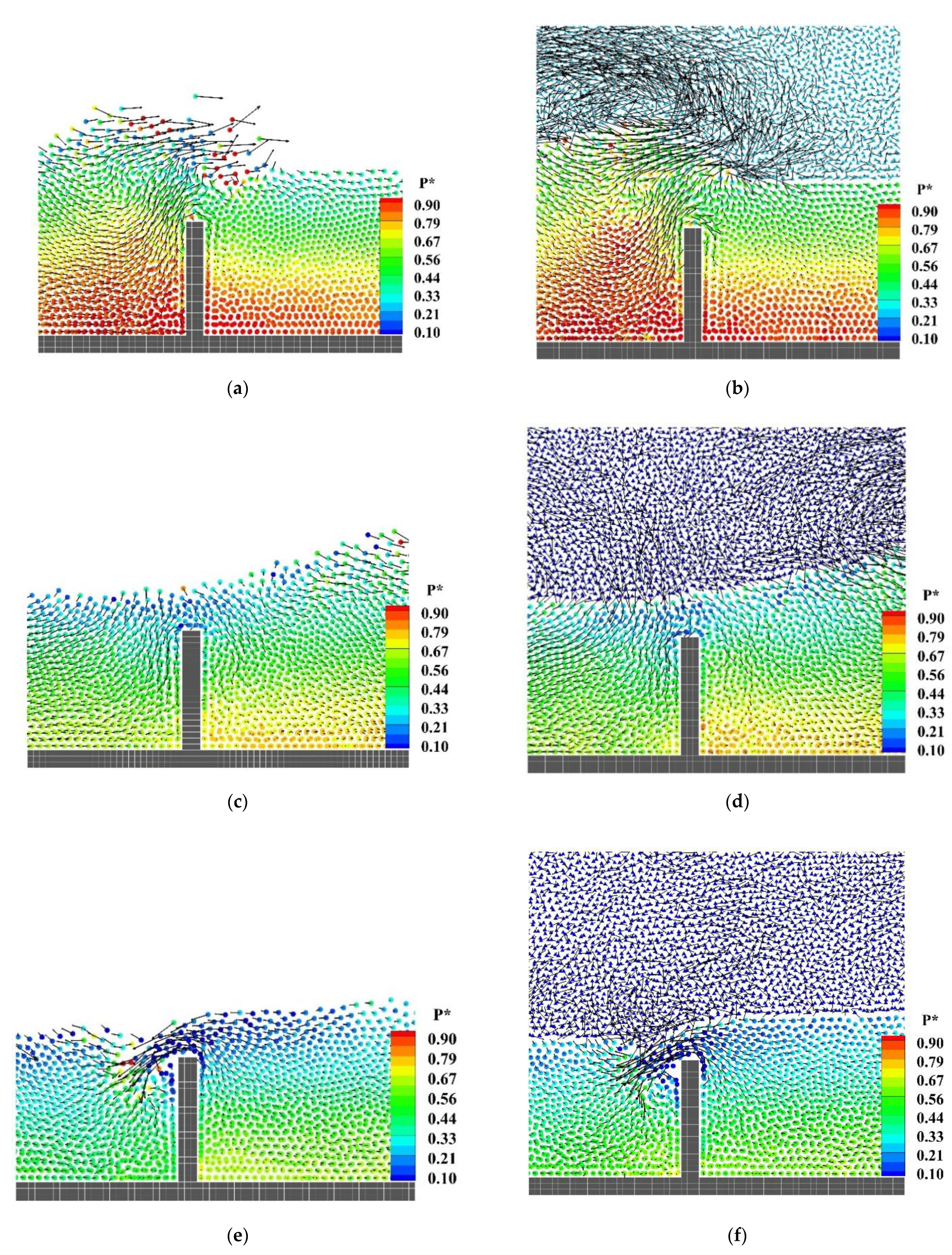
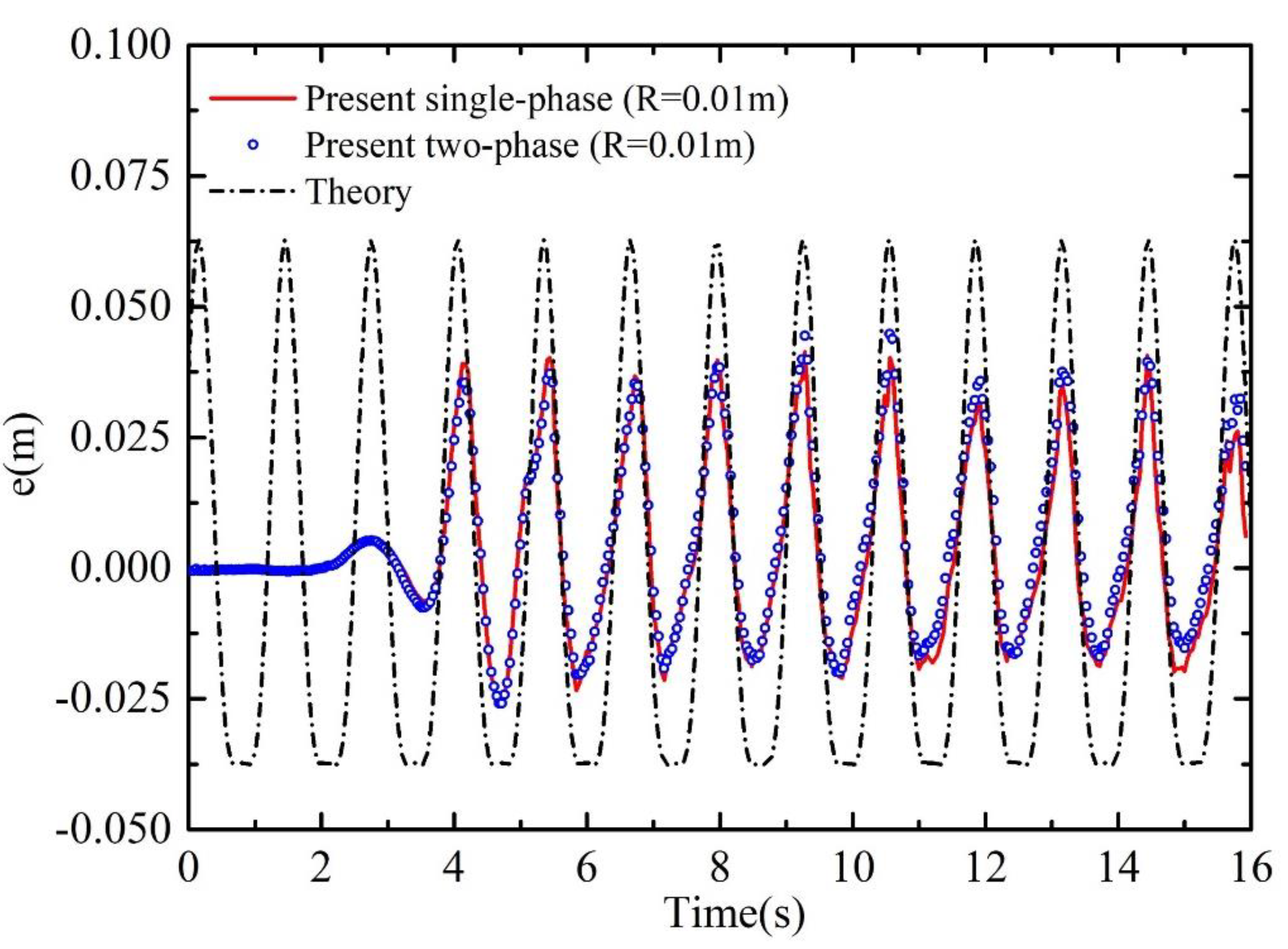
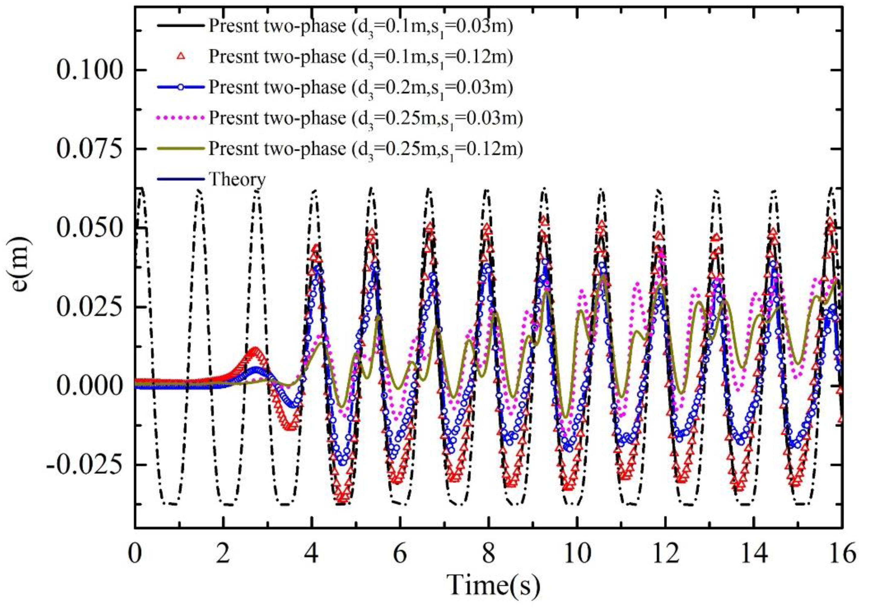
3.3. Two-Phase SPH Simulation of the Wave-Rigid Beam Interaction

The interaction of the waves created in the wave basin with a rigid cantilever beam fixed perpendicularly to the base of the wave basin and downstream of the wavemaker is addressed in this section. As shown in Figure 8, a rigid structure is set in the water, which is activated here to consider the WSI problem. The rigid cantilever beam of 0.2 m height and 0.03 m thickness is located at 2.8 m from the initial position of the piston wavemaker. The height of the beam can be changed to allow it to be submerged below the wavy interface or to protrude the wavy interface. A pressure sensor is placed at the height of 0.1 m (i.e., at half of the beam height). A second-order regular wave is generated using the same parameters and SPH settings and number of particles as outlined in Section 3.2. Figure 13 compares the temporal variation of the non-dimensional pressure P* = (P/(ρ₀ gd)) recorded by this pressure sensor computed using the single-phase and two-phase SPH simulations using the resolution R = 0.01 m developed in this study and also with that predicted using the single-phase mode in DualSPHysics using resolutions R = 0.01 m and 0.005 m.

During the initial stages of the wave generation, the pressure recorded at the sensor appears erratic. After 3 s when the waves are fully developed, there appears to be some temporal quasi-periodicity of the non-dimensional pressure and with a period of about 1.3 s. There appears to be no significant differences between the pressure variations computed using the present single-phase and two-phase SPH simulations, indicating that the effect of the air phase on the submerged structure may be negligible.

Three representative time instants t₁, t_2, and t₃ of 12.2 s, 12.6 s, and 13 s, respectively, (as shown in Figure 13) were selected to plot and compare the instantaneous contours of the non-dimensional pressure in the vicinity of the rigid beam structure computed using the single- and two-phase SPH codes from the present study which are shown in Figure 14. A pressure peak is achieved at t₁ = 12.2 s when the wave crest passes over the structure’s top, as shown in Figure 14a,b. After this, it can be seen that the pressure drops gradually as the wave crest passes over the structure at t₂ = 12.6 s, and this can be seen in Figure 14c,d. Subsequently, as shown in Figure 14e,f, a temporary backflow can be seen to occur at t₃ = 13 s, thereby resulting in a decay of the non-dimensional pressure to the trough. Since the wave elevation after passing the structure is significant for assessing the equivalence of the effectiveness of a barrier for say coastal protection, the temporal evolution of the free wavy surface at wave gauge WG3 computed using the single- and two-phase SPH from the present study are compared with the theoretical result (without the rigid beam structure) in Figure 15 with the same resolution.

Figure 16 shows the impact of structural shape parameters such as thickness and height on the wave profile. After passing the structure, the wave appears to have a period of 1.3 s, consistent with that of the wave generated without the structure in the basin. The variation in the choice of structural parameters such as the height (d₃) and thickness (S₁) (different structural sizes) can be considered to assess the effectiveness of the structure for coastal protection. As shown in Figure 16, the wave height appears to decrease as the structure height (d₃) is increased. Increasing the thickness, i.e., S₁ = 0.12 m appears to have no impact on the temporal variation of the wave heights, probably because the beam is assumed rigid for this study, which may not be the case if the beam is assumed to be elastic.

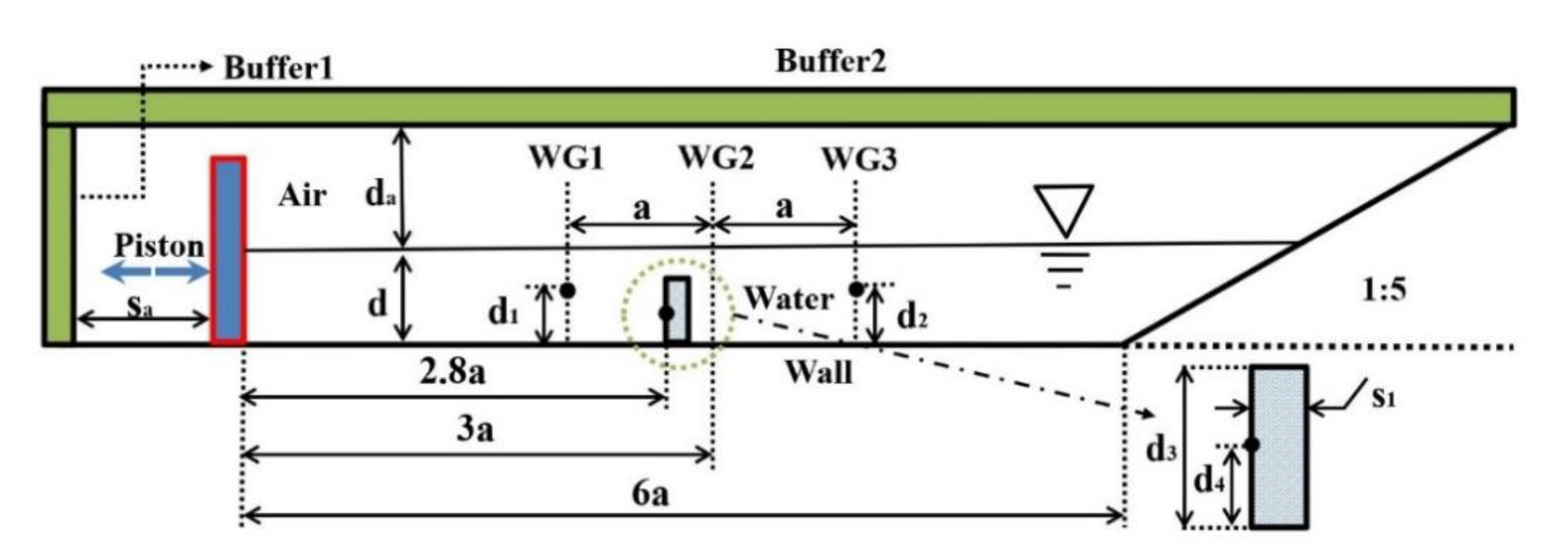
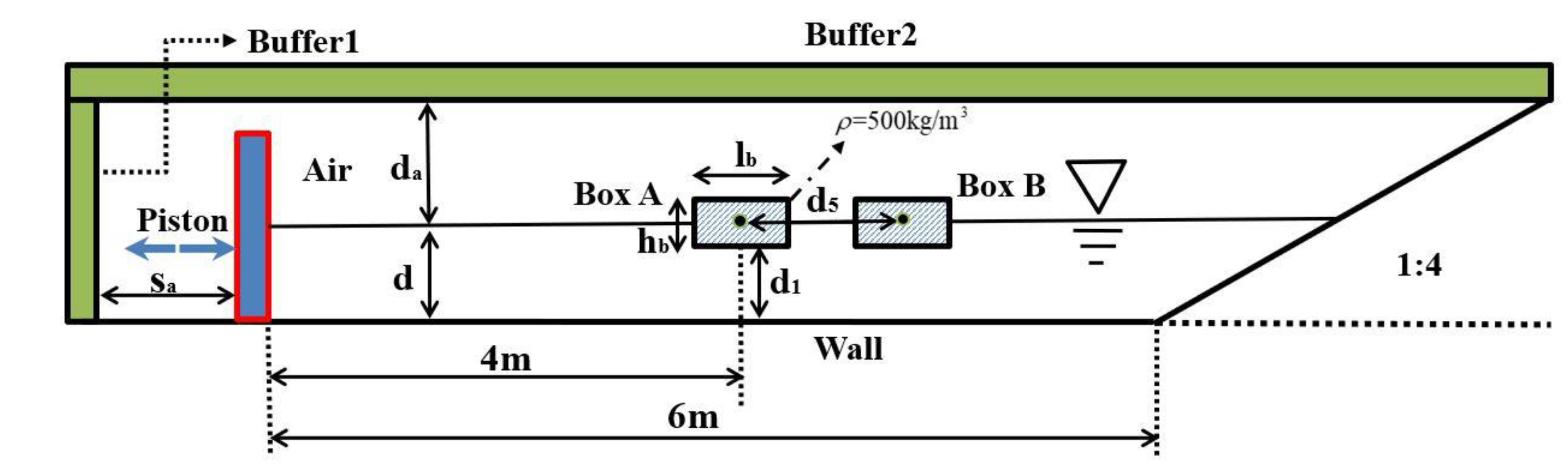
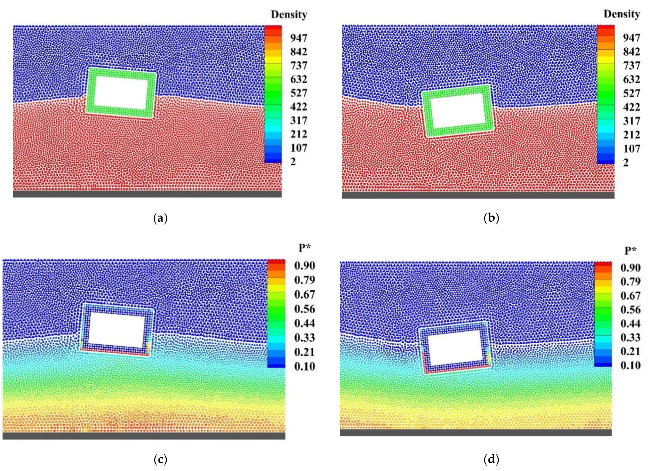
3.4. Two-Phase SPH Simulation of Wave Interaction with a Freely Floating Box in a Wave Basin

This section considers the hydrodynamic wave interaction with a freely floating rectangular box in the context of the present single- and two-phase SPH. This problem has already been experimented and simulated using single-phase SPH by Ren et al. [42] and Domínguez et al. [43] using DualSPHysics.

Figure 17 shows a schematic of the test problem showing a freely floating box (Box A) with a length l_b of 0.3 m, a height h_b of 0.2 m, and unit width in the spanwise direction in the wave basin (Box B will be activated in the next section). The box with a density of 500 kg/m³ is initially half-submerged in the water and then activated by a wave generated from the wavemaker with a period T of 1.2 s and a wave height H₀ of 0.1 m. The effect of this will be to cause the freely floating box to move in the direction (surge) and perpendicular to the direction (heave) of wave propagation and the rotation (pitch) concerning the mass center (counter-clockwise is positive). The wavemaker generates a second-order Stokes wave in the basin, and the waves are absorbed in the 1:4-sloped dissipative beach at the end of the basin. No-slip boundary conditions are implemented on the bottom wall and the dissipative beach. Buffers 1 and 2 denote the open boundaries treated as discussed in Section 3.2 and Section 3.3. Other numerical parameters remain the same as those mentioned in Section 3.3 if these are not specified. The total number of particles used for single-phase SPH is 70023 and for the two-phase SPH is 32770. A resolution of 0.01 m suggested in [42] is used in the present study. The computed temporal variation of heave, surge, and pitch for the floating box using single- and two-phase SPH from the present study are shown in Figure 18, respectively, and are compared with the experimental data for the same problems from [42]. Comparing the results between single-phase and two-phase simulations, the observed slight differences indicate that the single-phase model is better than the two-phase model to reflect the two-phase wave-floating structure interaction problem when the air is still in the infinite field. Still, we find that the single-phase model induces a slightly greater fluctuation of the box than the two-phase one. Figure 19a,d shows the computed contours of the density and the non-dimensional pressure $\overline{P}$ = P/(ρ₀ gd)) using the two-phase SPH of the present study at two selected times instants of t₁ and t₂ of 6.1 s and 6.8, respectively, as indicated in Figure 18a. It can be seen that the air-water interface in the vicinity of the box is captured clearly, and the box bobs up as shown in Figure 19c with higher pressure at the bottom of the wave basin than when it bobs down as shown in Figure 19d.

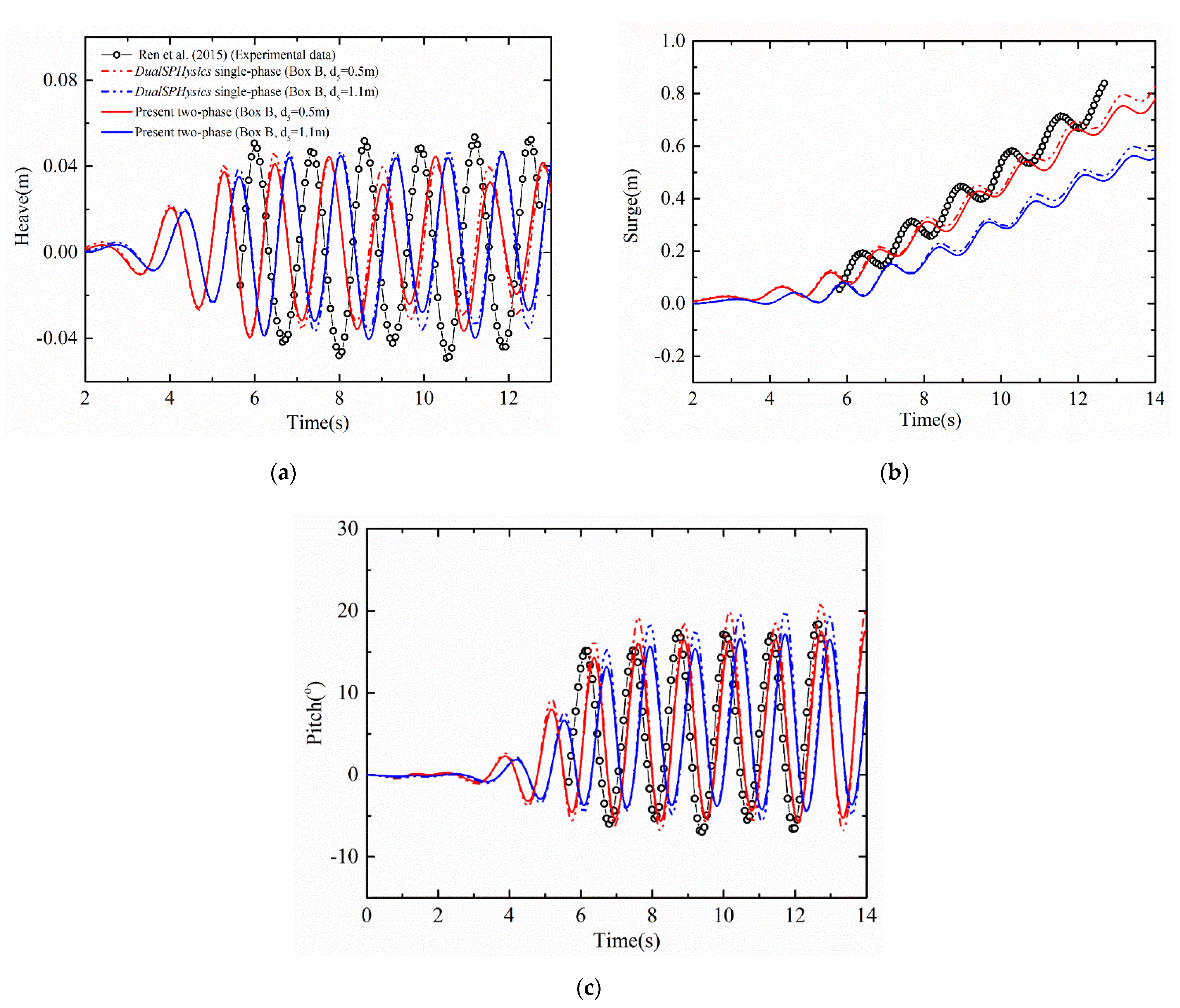
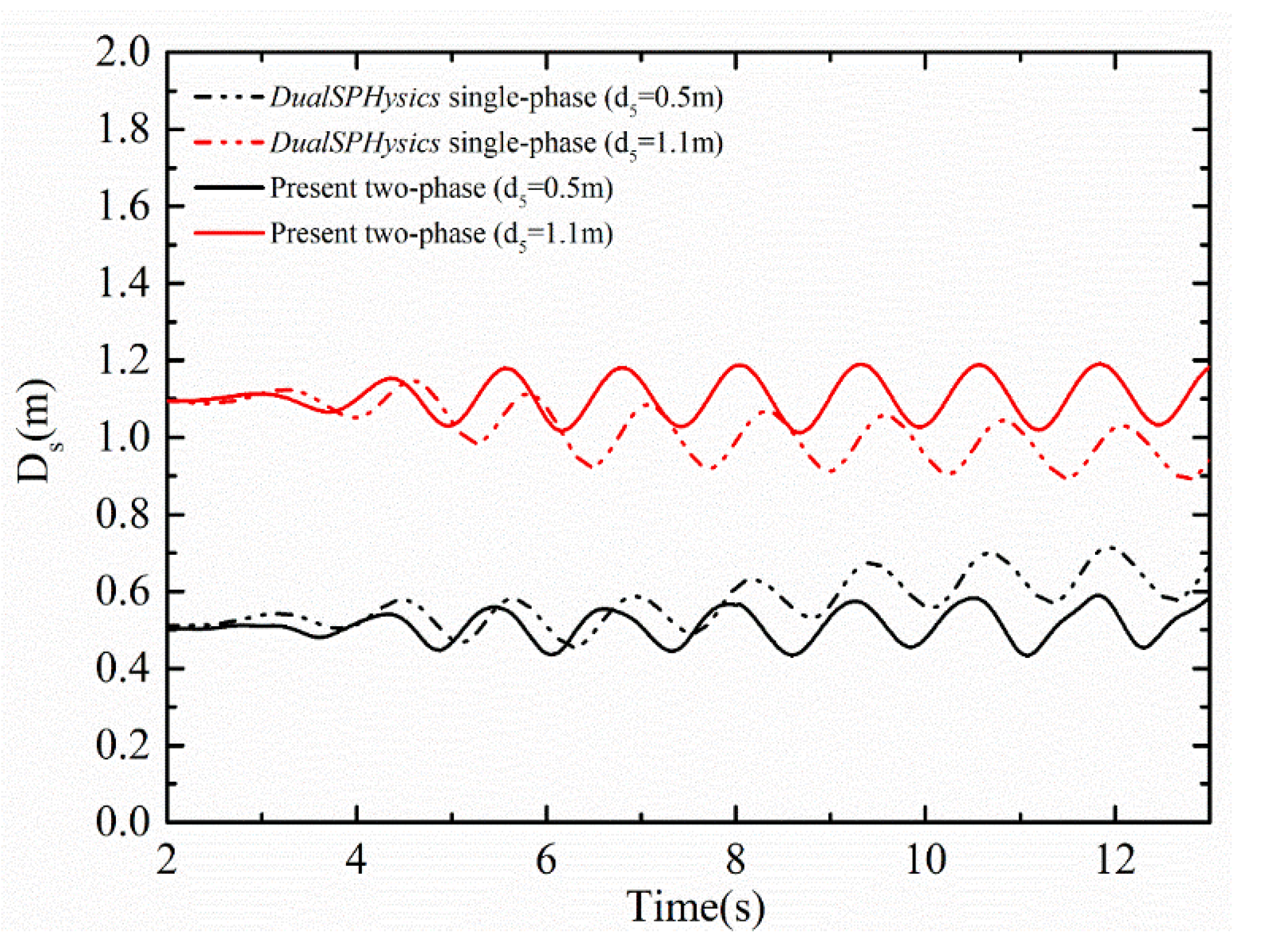
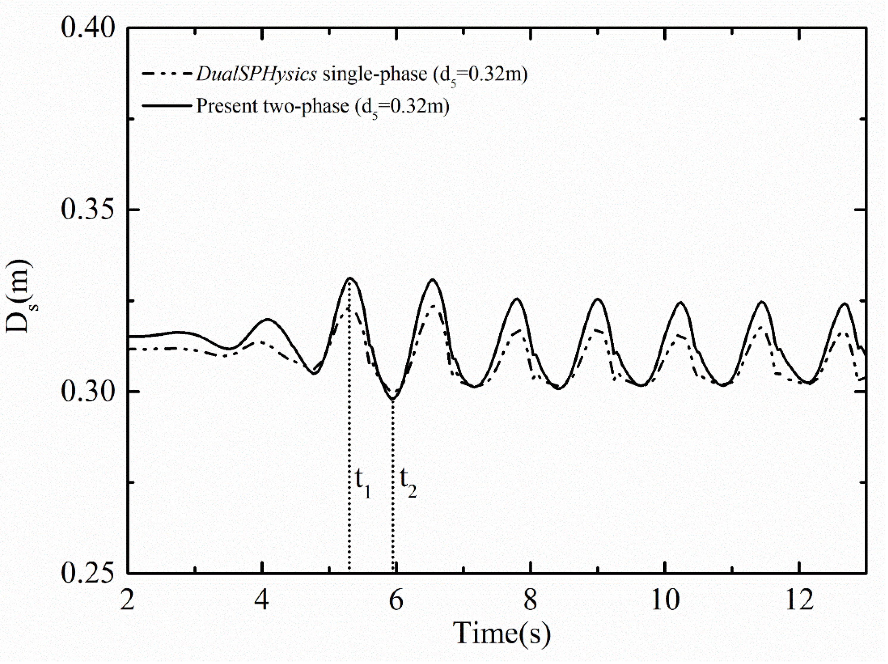
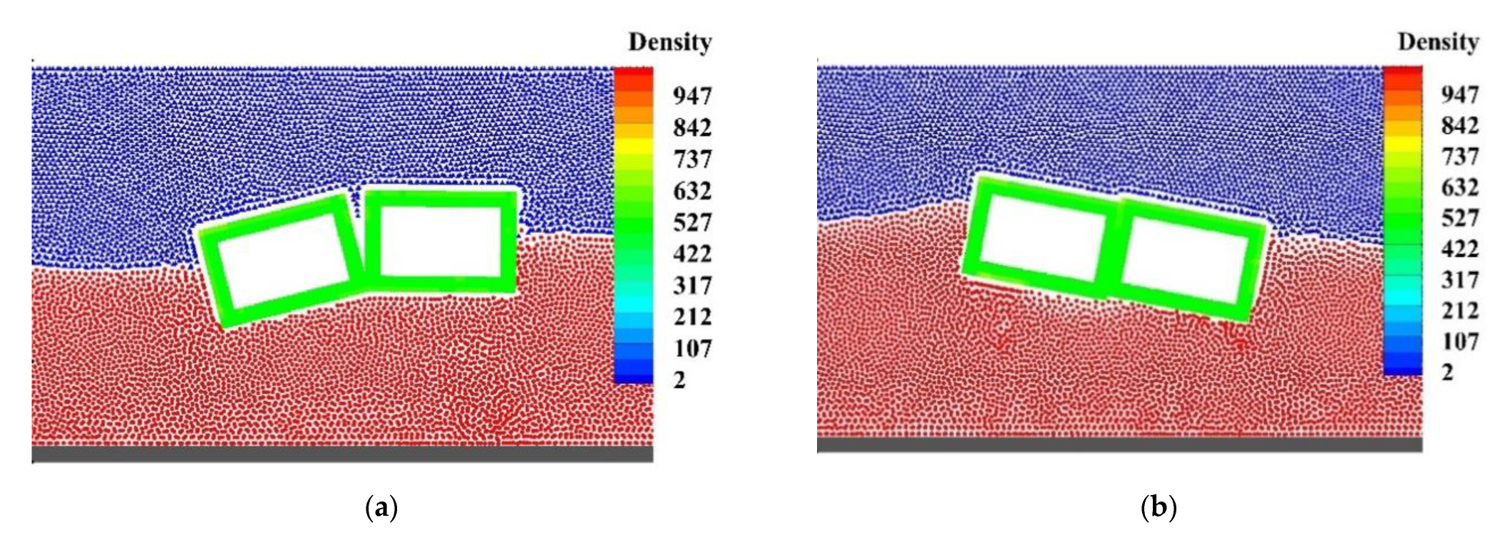
3.5. Wave Interaction with Two Freely Floating Boxes in a Basin

In this section, two freely floating boxes in the wave basin are investigated. This problem has not been fully resolved numerically due to the complexity of combining two-phase flow, WSI, and the collisions between the two boxes. Here, we release a box (Box A) as in Section 3.4 and add an extra box (Box B) behind it (initially half-submerged in the water, see Figure 17), with an initial distance of d₅ from the mass center of Box B to that of Box A. The two boxes maintain the length of 0.3 m, the height of 0.2 m, and the density of 500 kg/m³. The resolution of 0.01 m is adopted for our two-phase simulations. The other simulation setup remains the same, as indicated in Figure 17. By varying the location of Box B, two relative distances, i.e., d₅ = 0.5 m and 1.1 m, are initially given, corresponding to the motion of the two boxes as plotted in Figure 20 and Figure 21. Note that the experimental data of a single box (Box A) in the reference [42], and single-phase simulation (two boxes) results obtained using DulSPHysics with a resolution of 0.007 m are plotted here for a better comparison. For Box A with a greater initial distance (1.1 m) to Box B, the effect of Box B on the motion of Box B can be neglected (compare to single box simulation results). On a smaller initial distance (0.5 m), Box A is hindered by the hydrodynamic interaction with Box B in the direction (surge) of wave propagation (see Figure 20 b). Regarding Box B, it is observed that the heaving amplitude is somewhat smaller than that of a single box (compare to the experiment data), as shown in Figure 21a, indicating that some wave energy is dissipated by Box A. It is observed that Box B with a smaller initial distance (0.5 m) to Box A presents a more significant surging displacement than that of the case with a greater one. This can be explained as the smaller initial distance contributes to a more vital hydrodynamic interaction in pushing Box B (Figure 21b) and hindering Box A (see Figure 20b) in the surging direction. Figure 22 presents the time evolution for the relative distances between the two boxes with different initial locations in which the final distances tend to remain stable periods. The differences between our two-phase simulation results and those single-phase results obtained using DualSPHysics may result from the existence of the air phase.

Since the initial distances aforementioned are too large to collide, a significantly smaller initial distance, i.e., d₅ = 0.32 m, is adopted for considering the collision between the two boxes. The collision force model adopted here has been addressed as outlined in Section 2.4. After the collision for the first time, the two boxes remain attached, corresponding to the coincidence of peaks in the surge direction as shown in Figure 23b. The variation of the relative distance and the motion for the two boxes reflects a typical interaction process in which the two boxes collide with each other, periodically taking the contact points as the fulcrum. This process is clearly described through the two snapshots at t₁ = 5.3 s and t₂ = 5.95 s (see Figure 24), as shown in Figure 25.

4. Conclusions

In this paper, an SPH method was used to simulate several two-phase WSI examples. We validate a two-phase dam-breaking and a second-order wave generated by a piston in a wave basin to capture the wavy air-water interface, and the interaction between the wave and a floating box. Subsequently, we first studied the interaction between the wave and a rigid cantilever beam, and the interaction between the wave and two identical floating boxes with the possibility of elastic collision between them.

For the dam-breaking case, a smoother cavity interface was observed due to the weak compressibility of the local air phase for the two-phase simulation. Without the air phase, the cavity collapses due to the pressure difference between its top and bottom. The pressure evolution of a sensor on the right wall using single- and two-phase SPH simulations shows agreement with the experimental data and the available numerical results, indicating that our numerical model can provide a reliable solution to this problem. Based on the Biesel transfer function theory, the two-phase and second-order regular wave is generated by moving a piston in a wave basin and implementing the open boundary condition at the top and left of the domain of the air phase. The obtained wave elevation evolution and the velocity components using the single- and two-phase SPH at the wave gauges match the theoretical solution and those obtained by the single-phase DualSPHysics to a reasonable extent. Even though the same velocity patterns and free-surface profiles were observed for the one- and two-phase simulation in a global sight, the air phase can smooth the water-air interface by complementing the particles for the calculation in the vicinity of the water surface area where the particle supporting domain is truncated for the single-phase problem. The effect of different structural sizes on the wave elevation was investigated, and it was found that the increase of structure height decreases the wave elevation. On the motion of a floating box in the presence of the wave, our results show an agreement with the available experimental data, and only slight differences have been observed between the single- and two-phase simulations. On the motion of two floating boxes in the wave, it is observed that Box B with a smaller initial distance (0.5 m) to Box A presents a more significant surging displacement than that of the case with a greater one, which can be explained as the smaller initial distance contributes to a stronger hydrodynamic interaction in pushing Box B and hindering Box A in the surging direction. For the case of collision between the two boxes, we find that the two boxes collide periodically with taking the contact points as the fulcrum.

References

1. Huang, Z.; Li, Y.; Liu, Y. Hydraulic performance and wave loadings of perforated/slotted coastal structures: A review. Ocean. Eng. 2011, 38, 1031–1053. [Google Scholar] [CrossRef]
2. Lamas-Pardo, M.; Iglesias, G.; Carral, L. A review of very large floating structures (VLFS) for coastal and offshore uses. Ocean. Eng. 2015, 109, 677–690. [Google Scholar] [CrossRef]
3. Wang, C.; Tay, Z. Very large floating structures: Applications, research and development. Procedia Eng. 2011, 14, 62–72. [Google Scholar] [CrossRef] [Green Version]
4. Chakrabarti, S.K. (Ed.) Numerical Models in Fluid Structure Interaction, Advances in Fluid Mechanics; WIT Press: Southampton, UK, 2005; Volume 42. [Google Scholar]
5. Weymouth, G.; Dommermuth, D.G.; Hendrickson, K.; Yue, D.K.P. Advances in Cartesian-grid Methods for Computational Ship Hydrodynamics. In Proceedings of the 26th Symposium on Naval Hydrodynamics, Rome, Italy, 17–22 September 2006. [Google Scholar]
6. Chau, F.P.; Taylor, R.E. Second-order wave diffraction by a vertical cylinder. J. Fluid Mech. 1992, 240, 571. [Google Scholar] [CrossRef]
7. Stansberg, C.T.; Kristiansen, T. Non-linear scattering of steep surface waves around vertical columns. Appl. Ocean. Res. 2005, 27, 65–80. [Google Scholar] [CrossRef]
8. Walker, D.; Eatock Taylor, R.; Taylor, P.; Zang, J. Wave diffraction and near-trapping by a multi-column gravity-based structure. Ocean. Eng. 2008, 35, 201–229. [Google Scholar] [CrossRef]
9. Zang, J.; Gibson, R.; Taylor, P.H.; Eatock Taylor, R.; Swan, C. Second order wave diffraction around a fixed ship-shaped body in unidirectional steep waves. J. Offshore Mech. Arct. Eng. 2006, 128, 89–99. [Google Scholar] [CrossRef]
10. Hadžić, I.; Hennig, J.; Perić, M.; Xing-Kaeding, Y. Computation of flow-induced motion of floating bodies. Appl. Math. Model. 2005, 29, 1196–1210. [Google Scholar] [CrossRef]
11. Hu, C.; Kashiwagi, M. Two-dimensional numerical simulation and experiment on strongly non-linear wave–body interactions. J. Mar. Sci. Technol. 2008, 14, 200–213. [Google Scholar] [CrossRef]
12. Chen, L.; Zang, J.; Hillis, A.; Morgan, G.; Plummer, A. Numerical investigation of wave–structure interaction using OpenFOAM. Ocean. Eng. 2014, 88, 91–109. [Google Scholar] [CrossRef] [Green Version]
13. Hu, Z.Z.; Greaves, D.; Raby, A. Numerical wave tank study of extreme waves and wave-structure interaction using OpenFoam®. Ocean. Eng. 2016, 126, 329–342. [Google Scholar] [CrossRef] [Green Version]
14. Li, Y.; Ong, M.C.; Tang, T. A numerical toolbox for wave-induced seabed response analysis around marine structures in the OpenFOAM® framework. Ocean. Eng. 2020, 195, 106678. [Google Scholar] [CrossRef]
15. Lucy, L.B. A numerical approach to the testing of the fission hypothesis. Astron. J. 1977, 82, 1013. [Google Scholar] [CrossRef]
16. Gingold, R.A.; Monaghan, J.J. Smoothed particle hydrodynamics: Theory and application to non-spherical stars. Mon. Not. R. Astron. Soc. 1977, 181, 375–389. [Google Scholar] [CrossRef]
17. Ni, X.Y.; Feng, W.B. Numerical simulation of wave overtopping based on DualSPHysics. Appl. Mech. Mater. 2013, 405, 1463–1471. [Google Scholar] [CrossRef]
18. Wen, H.; Ren, B.; Dong, P.; Wang, Y. A SPH numerical wave basin for modeling wave-structure interactions. Appl. Ocean. Res. 2016, 59, 366–377. [Google Scholar] [CrossRef] [Green Version]
19. Altomare, C.; Domínguez, J.; Crespo, A.; González-Cao, J.; Suzuki, T.; Gómez-Gesteira, M.; Troch, P. Long-crested wave generation and absorption for SPH-based DualSPHysics model. Coast. Eng. 2017, 127, 37–54. [Google Scholar] [CrossRef]
20. Meringolo, D.D.; Aristodemo, F.; Veltri, P. SPH numerical modeling of wave–perforated breakwater interaction. Coast. Eng. 2015, 101, 48–68. [Google Scholar] [CrossRef]
21. Huang, C.; Zhang, D.; Si, Y.; Shi, Y.; Lin, Y. Coupled finite particle method for simulations of wave and structure interaction. Coast. Eng. 2018, 140, 147–160. [Google Scholar] [CrossRef]
22. Monaghan, J.J.; Lattanzio, J.C. A refined particle method for astrophysical problems. Astron. Astrophys. 1985, 149, 135–143. [Google Scholar]
23. Antuono, M.; Colagrossi, A.; Marrone, S. Numerical diffusive terms in weakly-compressible SPH schemes. Comput. Phys. Commun. 2012, 183, 2570–2580. [Google Scholar] [CrossRef]
24. Hu, X.; Adams, N. An incompressible multi-phase SPH method. J. Comput. Phys. 2007, 227, 264–278. [Google Scholar] [CrossRef]
25. Monaghan, J.J. Smoothed particle hydrodynamics. Annu. Rev. Astron. Astrophys. 1992, 30, 543–574. [Google Scholar] [CrossRef]
26. Morris, J.P.; Fox, P.J.; Zhu, Y. Modeling low Reynolds number incompressible flows using SPH. J. Comput. Phys. 1997, 136, 214–226. [Google Scholar] [CrossRef]
27. Aami, S.; Hu, X.; Adams, N. A generalized wall boundary condition for smoothed particle hydrodynamics. J. Comput. Phys. 2012, 231, 7057–7075. [Google Scholar] [CrossRef]
28. Tafuni, A.; Domínguez, J.; Vacondio, R.; Crespo, A. A versatile algorithm for the treatment of open boundary conditions in smoothed particle hydrodynamics GPU models. Comput. Methods Appl. Mech. Eng. 2018, 342, 604–624. [Google Scholar] [CrossRef]
29. Liu, M.; Liu, G. Restoring particle consistency in smoothed particle hydrodynamics. Appl. Numer. Math. 2006, 56, 19–36. [Google Scholar] [CrossRef]
30. Verlet, L. Computer “Experiments” on classical fluids. I. Thermodynamical properties of Lennard-Jones molecules. Phys. Rev. 1967, 159, 98–103. [Google Scholar] [CrossRef]
31. Newmark, N. A Method of Computation for Structural Dynamics. J. Eng. Mech. Div. 1959, 85, 67–94. [Google Scholar] [CrossRef]
32. Canelas, R.B.; Crespo, A.J.; Domínguez, J.M.; Ferreira, R.M.; Gómez-Gesteira, M. SPH–DCDEM model for arbitrary geometries in free surface solid–fluid flows. Comput. Phys. Commun. 2016, 202, 131–140. [Google Scholar] [CrossRef]
33. Kuwabara, G.; Kono, K. Restitution coefficient in a collision between two spheres. Jpn. J. Appl. Phys. 1987, 26, 1230–1233. [Google Scholar] [CrossRef]
34. Lemieux, M.; Léonard, G.; Doucet, J.; Leclaire, L.; Viens, F.; Chaouki, J.; Bertrand, F. Large-scale numerical investigation of solids mixing in a V-blender using the discrete element method. Powder Technol. 2008, 181, 205–216. [Google Scholar] [CrossRef]
35. Vetsch, F.D. Numerical Simulation of Sediment Transport with Meshfree Methods. Doctoral Dissertation, ETH Zurich, Zurich, Switzerland, 2012. [Google Scholar]
36. Gong, K.; Shao, S.; Liu, H.; Wang, B.; Tan, S. Two-phase SPH simulation of fluid–structure interactions. J. Fluids Struct. 2016, 65, 155–179. [Google Scholar] [CrossRef] [Green Version]
37. Chen, Z.; Zong, Z.; Liu, M.; Zou, L.; Li, H.; Shu, C. An SPH model for multiphase flows with complex interfaces and large density differences. J. Comput. Phys. 2015, 283, 169–188. [Google Scholar] [CrossRef]
38. Buchner, B. Green Water on Ship-Type Offshore Structures. Ph.D. Thesis, Delft University of Technology, Delft, The Netherlands, 2002. [Google Scholar]
39. Biesel, F.; Suquet, F. Etude theorique d’un type d’appareil a la houle. Houille Blanche 1951, 6, 152–165. [Google Scholar]
40. Frigaard, P.; Andersen, T. Technical Background Material for the Wave Generation Software AwaSys 5; Aalborg University: Aalborg, Denmark, 2010; Available online: https://core.ac.uk/display/60460686 (accessed on 6 February 2021).
41. Madsen, O.S. On the generation of long waves. J. Geophys. Res. 1971, 76, 8672–8683. [Google Scholar] [CrossRef]
42. Ren, B.; He, M.; Dong, P.; Wen, H. Non-linear simulations of wave-induced motions of a freely floating body using WCSPH method. Appl. Ocean. Res. 2015, 50, 1–12. [Google Scholar] [CrossRef]
43. Domínguez, J.M.; Crespo, A.J.; Hall, M.; Altomare, C.; Wu, M.; Stratigaki, V.; Troch, P.; Cappietti, L.; Gómez-Gesteira, M. SPH simulation of floating structures with moorings. Coast. Eng. 2019, 153, 103560. [Google Scholar] [CrossRef]
Figure 1. Schematic of an SPH particle in its support domain.
Energies 15 03251 g001
Figure 2. Schematic of the open boundary condition for the outflow. The translucent areas denote the supporting domains. The mirror particles are mirrored by the ghost particles concerning the outflow threshold. (a) wall boundary, the pressure on the solid particle i is extrapolated from the neighboring fluid particle j; (b) open boundary, the physical information (pressure, density, or velocity) at a ghost particle is calculated (Equation (7)) using that of the mirror particles; the information of a mirror particle is interpolated (Equation (6)) from that of the fluid particles in its supporting domain.
Energies 15 03251 g002
Figure 3. Schematic of DEM collision. The red dots denote the mass centers of the two boxes; the black dots denote the collision points of the two boxes.
Energies 15 03251 g003
Figure 4. Schematic of a multiphase dam-breaking.
Energies 15 03251 g004
Figure 5. Comparison of single- and two-phase SPH results with that of Chen et al. [37] for dam-breaking flow at dimensionless time t(g/H)0.5 = 6.4. The hollow “triangles” and “diamonds” denote the surfaces of the water obtained from the present single-phase simulation and reference [37], respectively. The blue solid “dots” denote the water particles, in which the air phase has been hidden for a distinct water-air interface.
Energies 15 03251 g005
Figure 6. Comparison of pressure for two-phase SPH simulation of dam-breaking flow at dimensionless time t(g/H)0.5 = 6.4. (a) present study; (b) study of Chen et al. [37]. The measurement unit is m in the x- and y-axis.
Energies 15 03251 g006
Figure 7. Comparison of the time variations of dimensionless pressure. The experimental data and the available numerical results are respectively from Buchner [38] and Chen et al. [37].
Energies 15 03251 g007
Figure 8. Schematic of the computational domain for the 2D wave basin.
Energies 15 03251 g008
Figure 9. Comparison of theoretical and numerical free surface elevations at different wave gauges for the wave generation study. (a) x = 2 m; (b) x = 4 m.
Energies 15 03251 g009
Figure 10. Comparison of theoretical and numerical orbital velocities at the velocity gauge (x = 4 m, d2 = 0.12 m) for the wave generation study. (a) Ux; (b) Uy.
Energies 15 03251 g010
Figure 11. Snapshot of the horizontal velocity component for one-phase and two-phase wave generation studies at t = 16 s. (a) single-phase; (b) two-phase. Here (c,d) correspond to the enlarged (a,b) at mark 1 and mark 2, respectively.
Energies 15 03251 g011aEnergies 15 03251 g011b
Figure 12. Snapshot of the density for two-phase wave generation study at t = 16 s. Here (b,c) correspond to the enlarged image of (a) and the horizontal velocity and the vectors at mark 1, respectively. The magnitude of the vectors indicates the strength of the flows.
Energies 15 03251 g012
Figure 13. Time evolution of the dimensionless pressure on the sensor of the structure for single-phase and two-phase wave generation studies.
Energies 15 03251 g013
Figure 14. Snapshot of the dimensionless pressure in the vicinity of the structure for single-phase and two-phase wave generation studies. (a) single-phase flow (t1 = 12.2 s); (b) two-phase flow (t1 = 12.2 s); (c) single-phase flow (t2 = 12.6 s); (d) two-phase flow (t2 = 12.6 s); (e) single-phase flow (t3 = 13 s); (f) two-phase flow (t3 = 13 s). The magnitude of the vectors indicates the strength of the flows.
Energies 15 03251 g014
Figure 15. Single- and two-phase SPH computed temporal evolution of the free surface at WG3 immediately after the wave has passed the structure.
Energies 15 03251 g015
Figure 16. Comparison of the present single- and two-phase SPH computed temporal evolution of the free surface at WG3 immediately after the wave has passed the structure with different geometrical sizes computed using SPH code and theory without the structure in the basin.
Energies 15 03251 g016
Figure 17. Schematic of initial location for a freely floating box in the 2D two-phase wave basin. Box B will be activated in the next section.
Energies 15 03251 g017
Figure 18. Comparison with the experimental data [42] for the motion of the freely floating box under the action of regular waves. (a) heave; (b) surge; (c) pitch.
Energies 15 03251 g018
Figure 19. Different time instants for the freely floating box under the action of regular waves. (a) density (t1 = 6.1 s); (b) density (t2 = 6.8 s); (c) pressure (t1 = 6.1 s); (d) pressure (t2 = 6.8 s).
Energies 15 03251 g019
Figure 20. Comparisons of time evolution with different initial distance d5 for the heave (a), surge (b), and pitch (c) of Box A under the action of regular waves. The available experimental results are from Ren et al. [42].
Energies 15 03251 g020
Figure 21. Comparisons of time evolution with different initial distance d5 for the heave (a), surge (b), and pitch (c) of Box B under the action of regular waves. The available experimental results are from Ren et al. [42].
Energies 15 03251 g021
Figure 22. Comparisons of time evolution with different initial distance d5 for the relative distance between the two boxes under the action of regular waves.
Energies 15 03251 g022
Figure 23. Motion for the two boxes with collision under the action of regular waves. (a) heave; (b) surge; and (c) pitch.
Energies 15 03251 g023
Figure 24. Relative distance for the two boxes with collision under the action of regular waves.
Energies 15 03251 g024
Figure 25. Different time instants for the collision of the two boxes under the action of regular waves. (a) t1 = 5.3 s; (b) t2 = 5.95 s.
Energies 15 03251 g025
Publisher’s Note: MDPI stays neutral with regard to jurisdictional claims in published maps and institutional affiliations.