
Low and Ultra-Low Temperature District Heating Equipped by Heat Pumps—An Analysis of the Best Operative Conditions for a Swiss Case Study


Abstract
:1. Introduction
1.1. Low-Temperature DHS
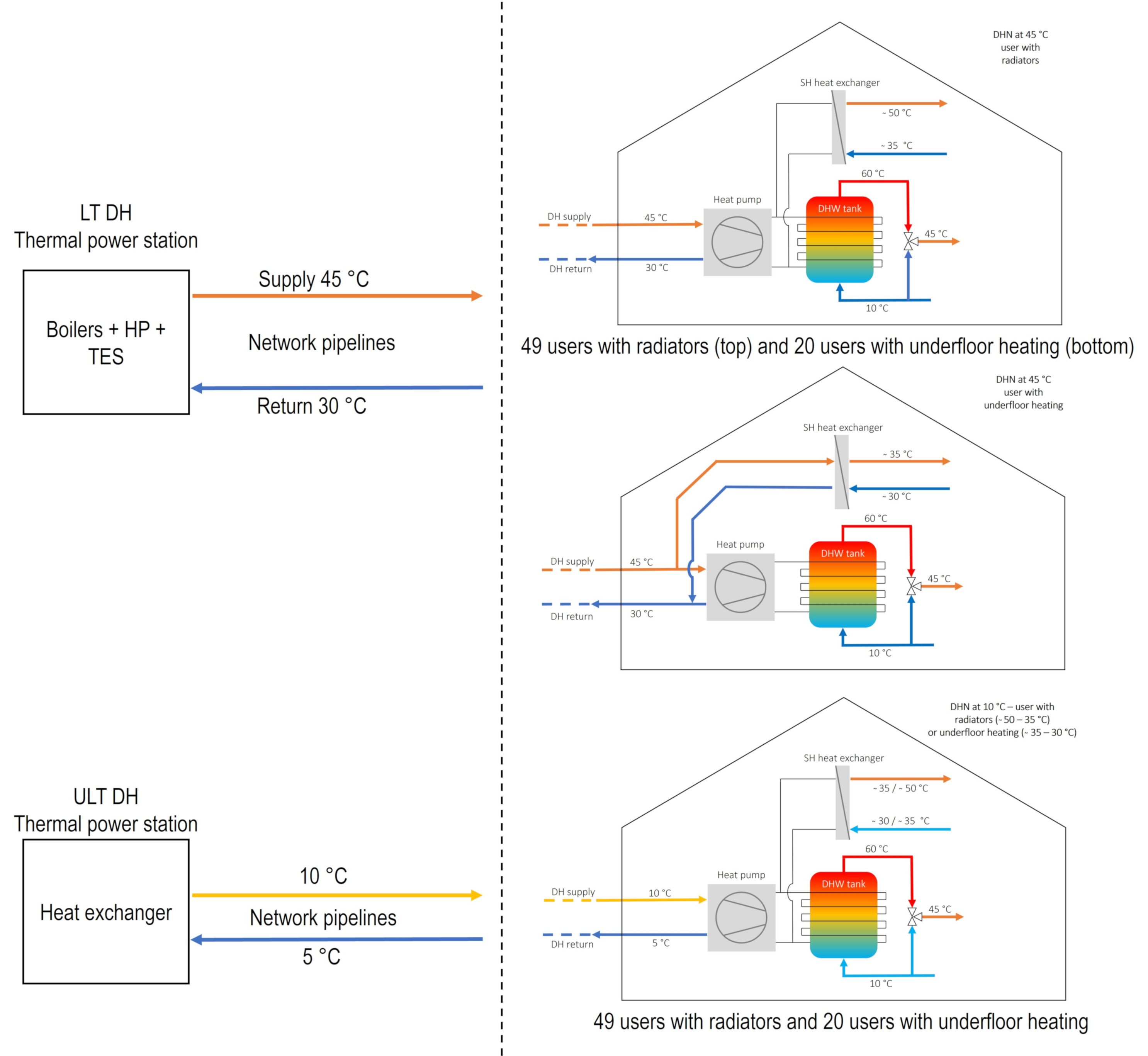
- Heat exchangers users’ side in case of radiant panels as an emitting system in the buildings and local HP devoted only to DHW;
- HP devoted to space heating and DHW users’ side in case of radiators as an emitting system in the buildings.
1.2. Ultra-Low Temperature DHS
2. Materials and Methods
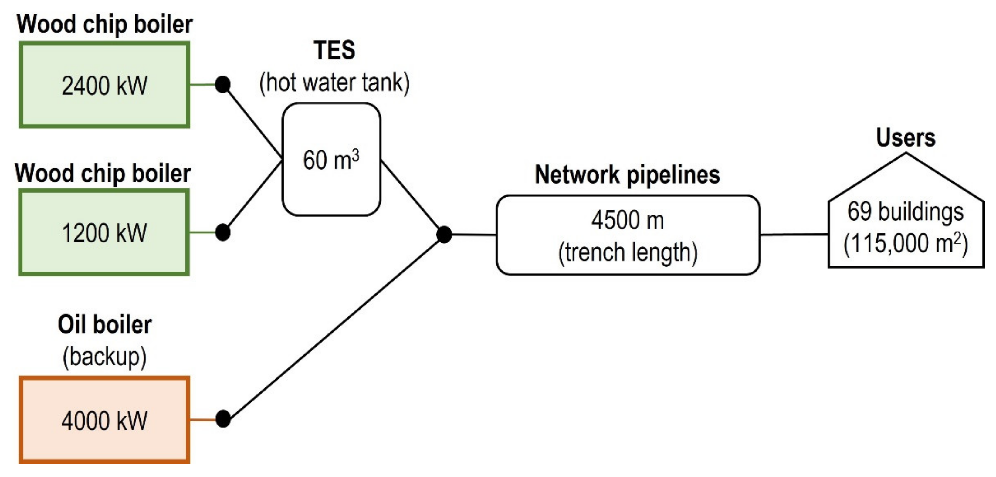
- An in-depth characterisation of the thermal power station and its storage system (water tank), with a focus on the performance of the HP, especially its electricity consumption at full and partial load at different operating conditions;
- A detailed simulation of DHN focusing on the thermal inertia of the network and the propagation delay of the temperature, based on a pseudo-dynamic model;
- A resistive—capacitive (R-C) model of the buildings connected to the DHN, allowing the dynamic simulation of the thermal demand according to the external climate data (Typical Meteorological Year—TMY file) and to the indoor comfort conditions;
- A completely-mixed model of the DHW tank to include the inertia offered by this storage system.
2.1. Description of Model
- Thermal power station: Heat Exchanger (HE) for ULT DHS; Heat Pump (HP) for LT DHS;
- Thermal energy storage (TES);
- Distribution network, equipped with a double pipeline, with different diameters of pipes;
- Thermal substations to the users: Heat Exchangers (HE); Heat Pumps (HP) for heating and for DHW purposes; Thermal storage for DHW purposes;
- Management and control system.
2.1.1. Model of the Heat Pumps
2.1.2. Model of the Distribution Networks
- As topology a tree network is considered;
- The carrier is water, considered an incompressible fluid with physical characteristics that are constant in time and uniform in space;
- The fluid flow is considered one-dimensional;
- The properties of the materials of the pipe, insulation, and soil are constant in time, uniform in space, and independent of temperature.
2.1.3. Model of the District Thermal Needs
- Thermal resistance of the envelope;
- Thermal capacity;
- SH peak power;
- DHW need in litres per day;
- Thermal resistance and capacity of the DHW storage;
- DHW peak power for the storage recharge.

| Thermal Power Station | References |
|---|---|
| Heat pump | [21,24,25] |
| Central pump | [22,23,32] |
| Central hot water tank | [14,15] |
| Network | |
| Network pipelines | [33,34] |
| Hydraulic and thermal resolution | [12,32,35,36,37] |
| Substations | |
| Building model | [25,26,27] |
| DHW tank model | [19,20,31] |
| Emitting system | [38,39] |
| Heat exchanger | [22,23,24,25,26,27,28,29,30,31,32,33,34,38] |
| Heat pump | [24,25,26,27] |
2.2. Definition of the Main Parameters Determining the DHS Features and Management
- The dynamics of the energy demand for SH and DHW for all the buildings connected to the thermal network, based on the local climatic conditions, the thermo-physic features of the buildings, and the needs for DHW;
- The different TES available, whether they are at the thermal power station or distributed to the users.
- Thermal power requested by the users;
- Thermal power requested from the thermal power station;
- Electric power requested by the HP decentralised to the buildings (users);
- Electric power requested by the HP in the thermal power station;
- Electric power requested by pumps and auxiliaries;
- Set point temperature to the users;
- Temperature levels of the thermal storage for the DHW supply.
2.3. Definition of Optimised Control Strategies for the Operation of the DHS
- Temperature levels of the DHN;
- TES volume at the thermal power station;
- Thermal resistance (R) and capacity (C) of the buildings’ envelope. Compatibly with the features of the existing building stock, in the beginning, different R and C were set in the simulations in order to observe the effects on the electric demand for the operation of the DHS. However, these parameters were not considered in the final results because the definition of scenarios with their improvement implies a general and uniform retrofit of the building stock that is not feasible in a short time;
- Set point temperature inside the buildings and its throttling range. Different set point temperatures and throttling ranges are set in the simulations in order to observe the effects on the electric demand for the operation of the DHS;
- Thermal R and C of the DHW storage, considering that the DHW needs to represent about the 20% of the total thermal needs, on a yearly basis;
- Operation conditions and performance of the HP users’ side, with particular regard to the operation in partial loads and to the shutdown.
2.3.1. Definition of the Scenarios
- Base case: the LT and ULT DHS are simulated according to the assumptions previously described considering a night set back: inside the buildings, a set point temperature of 19 °C instead of 21 °C is applied to all the users of the DHS, from 10 pm to 6 am. The Base case keeps the operative modality of the existing DHS and is useful to understand the effects of the substitution of the existing biomass systems by the two related to the LT and ULT configuration based on HP;
- Case 1: this case operates on the set point temperature inside the buildings. Case 1 is the same as Base case, but without night set back; in this case, the set point temperature is 21 °C all over the day;
- Case 2: this case operates on the shutdown of the HP and on the set point temperature inside the buildings. Case 2 is the same as Case 1, but with HP switched off for the most impacting consumers when the electric grid is under stress. Indeed seven users of the DHS account for the 41% of the thermal installed power (chosen as the users above the 90th percentile of the installed thermal power), while the electric grid is considered under stress when the power load is greater or equal to the 90th percentile of the electric peak observed in the base case;
- Case 3: this case operates on the set point temperature inside the buildings. Case 3 is the same as Case 1, but with set point temperature inside the buildings at 19 °C instead of 21 °C for the most impacting consumers when the electric grid is under stress.
3. Results
- Moving from the current HT DHS based on biomass and oil boiler as back up to the LT DHS based on HP, keeping the oil boiler as back up; the existing biomass boilers are substituted by two HP;
- Moving from the current HT DHS based on biomass and the oil boiler as backup to the ULT DHS based only on the possibility to circulate cool water and to supply SH and DHW by local HP; the existing biomass and oil boilers are substituted by the HE.
Results Achieved for the LT and ULT DHS
- For the LT DHN, the heat losses along the network are in the range of 3–7% of the heat supplied and the energy requested for pumping is around 1–2% of the heat supplied;
- For the ULT DHN network, where temperatures are also adapted to the direct cooling of the building by means of a heat exchanger, heat losses along the network are negligible and energy requested for pumping is around 2–3% of the heat supplied.
4. Discussion
5. Conclusions
- The definition of control logics at the component level, more customised to the performance of the singular building and system (e.g., the shutdown of the HP based on the thermal inertia of each building);
- The implementation of real-time feedback on the impact of the HP on the electric network and with relative instantaneous modification of the management rules;
- An in-depth study of the charge and discharge cycles of the TES with the optimisation of the control system;
- A more in-depth characterisation of the thermal models of buildings;
- The introduction of the space cooling and the study of its impact that, due to the consequences of climate change, will become increasingly relevant even at these latitudes (both to increase users’ comfort and to reduce the load on the electric grid due to increasing use of inefficient refrigeration machines);
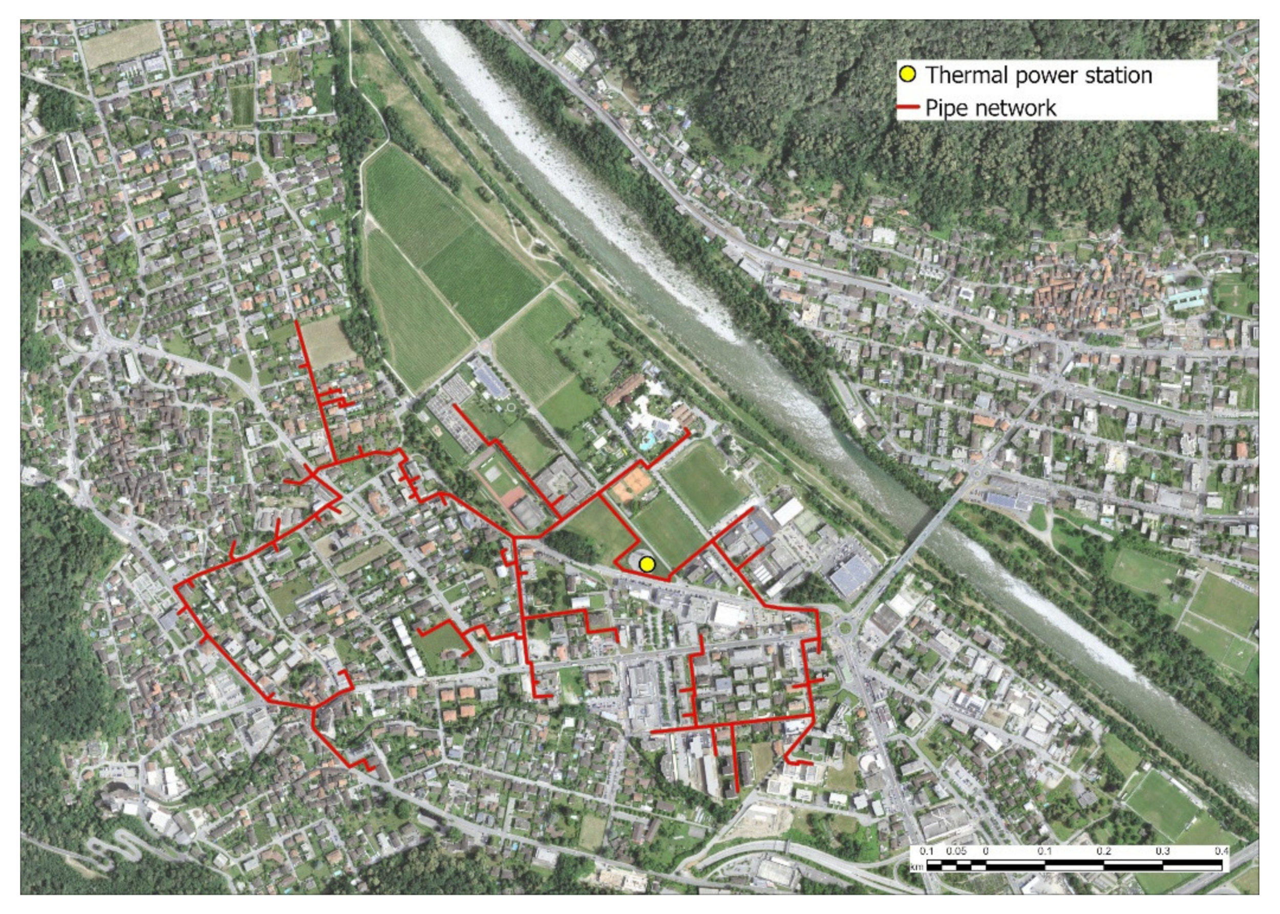
- A draft techno-economic evaluation of the feasibility of pertinent scenarios in the real case of Losone.
Author Contributions
Funding
Institutional Review Board Statement
Informed Consent Statement
Data Availability Statement
Acknowledgments
Conflicts of Interest
References
- Caputo, P.; Ferla, G.; Belliardi, M.; Cereghetti, N. District thermal systems: State of the art and promising evolutive scenarios. A focus on Italy and Switzerland. Sustain. Cities Soc. 2021, 65, 102579. [Google Scholar] [CrossRef]
- Lund, H.; Østergaard, P.A.; Nielsen, T.B.; Werner, S.; Thorsen, J.E.; Gudmundsson, O.; Arabkoohsar, A.; Mathiesen, B.V. Perspectives on fourth and fifth generation district heating. Energy 2021, 227, 120520. [Google Scholar] [CrossRef]
- FLEXYNETS: Fifth Generation, Low Temperature, High Exergy Heating and Cooling Network. Available online: http://www.flexynets.eu (accessed on 20 March 2022).
- Buffa, S.; Cozzini, M.; D’Antoni, M.; Baratieri, M.; Fedrizzi, R. 5th generation district heating and cooling systems: A review of existing cases in Europe. Renew. Sustain. Energy Rev. 2019, 104, 504–522. [Google Scholar] [CrossRef]
- Buffa, S.; Soppelsa, A.; Pipiciello, M.; Henze, G.; Fedrizzi, R. Fifth-generation district heating and cooling substations: Demand response with artificial neural network-based model predictive control. Energies 2020, 13, 4339. [Google Scholar] [CrossRef]
- Sulzer, M.; Werner, S.; Mennel, S.; Wetter, M. Vocabulary for the fourth generation of district heating and cooling. Smart Energy 2021, 1, 100003. [Google Scholar] [CrossRef]
- David, A.; Mathiesen, B.V.; Averfalk, H.; Werner, S.; Lund, H. Heat Roadmap Europe: Large-Scale Electric Heat Pumps in District Heating Systems. Energies 2017, 10, 578. [Google Scholar] [CrossRef] [Green Version]
- Sayegh, M.A.; Jadwiszczak; Axcell, B.P.; Niemierka, E.; Bryś, K.; Jouhara, H. Heat pump placement, connection and operational modes in European district heating. Energy Build. 2018, 166, 122–144. [Google Scholar] [CrossRef]
- Østergaard, P.A.; Andersen, A.N. Booster heat pumps and central heat pumps in district heating. Appl. Energy 2016, 184, 1374–1388. [Google Scholar] [CrossRef]
- Vivian, J.; Emmi, G.; Zarrella, A.; Jobard, X.; Pietruschka, D.; De Carli, M. Evaluating the cost of heat for end users in ultra low temperature district heating networks with booster heat pumps. Energy 2018, 153, 788–800. [Google Scholar] [CrossRef]
- Hangartner, D.; Ködel, J.; Mennel, S.; Sulzer, M. Grundlagen und Erläuterungen zu Thermischen Netzen; Swiss Federal Office of Energy (SFOE): Bern, Switzerland, 2018. (In German) [Google Scholar]
- Nussbaumer, T.; Thalmann, S.; Jenni, A.; Ködel, J. Handbook on Planning of District Heating Networks; Energieschweiz, Swiss Federal Office of Energy (SFOE): Bern, Switzerland, 2018; Available online: http://www.verenum.ch/Dokumente/Handbook-DH_V1.0.pdf (accessed on 28 March 2022).
- Gadd, H.; Werner, S. 18—Thermal energy storage systems for district heating and cooling. In Advances in Thermal Energy Storage Systems; Cabeza, L.F., Ed.; Woodhead Publishing Series in Energy; Woodhead Publishing: Sawston, UK, 2015; pp. 467–478. [Google Scholar] [CrossRef]
- Romanchenko, D.; Kensby, J.; Odenberger, M.; Johnsson, F. Thermal energy storage in district heating: Centralised storage vs. storage in thermal inertia of buildings. Energy Convers. Manag. 2018, 162, 26–38. [Google Scholar] [CrossRef]
- Steen, D.; Stadler, M.; Cardoso, G.; Groissböck, M.; DeForest, N.; Marnay, C. Modeling of thermal storage systems in MILP distributed energy resource models. Appl. Energy 2015, 137, 782–792. [Google Scholar] [CrossRef] [Green Version]
- Federal Statistical Office. Federal Register of Buildings and Dwellings (RBD). Available online: https://www.bfs.admin.ch/bfs/en/home/registers/federal-register-buildings-dwellings.html (accessed on 20 February 2022).
- SIA 385/1. Plants for Domestic Hot Water in Buildings—General Basics and Requirements; SIA: Zurich, Switzerland, 2020; (In French, German and Italian). [Google Scholar]
- SIA 385/2. Plants for Domestic Hot Water in Buildings—Global Requirements and Sizing; SIA: Zurich, Switzerland, 2015; (In French, German and Italian). [Google Scholar]
- Knudsen, M.D.; Petersen, S. Model predictive control for demand response of domestic hot water preparation in ultra-low temperature district heating systems. Energy Build. 2017, 146, 55–64. [Google Scholar] [CrossRef]
- Toffanin, R.; Curti, V.; Barbato, M.C. Impact of Legionella regulation on a 4th generation district heating substation energy use and cost: The case of a Swiss single-family household. Energy 2021, 228, 120473. [Google Scholar] [CrossRef]
- Verhelst, C.; Degrauwe, D.; Logist, F.; Van Impe, J.; Helsen, L. Multi-objective optimal control of an air-to-water heat pump for residential heating. Build. Simul. 2012, 5, 281–291. [Google Scholar] [CrossRef]
- Stoecker, W.F. Industrial Refrigeration Handbook; McGraw-Hill Education: New York, NY, USA, 1998; Available online: https://www.accessengineeringlibrary.com/content/book/9780070616233 (accessed on 20 March 2022).
- Bell, I.H.; Wronski, J.; Quoilin, S.; Lemort, V. Pure and Pseudo-pure Fluid Thermophysical Property Evaluation and the Open-Source Thermophysical Property Library CoolProp. Ind. Eng. Chem. Res. 2014, 53, 2498–2508. [Google Scholar] [CrossRef] [Green Version]
- Controls, J. Sabroe HeatPAC Heat Pumps Performance Data. 2019. Available online: https://www.johnsoncontrols.com/fi_fi/-/media/jci/be/finland/heat-pumps/files/bts_sabroe_heatpac_en_eu.pdf (accessed on 25 March 2022).
- Fuentes, E.; Waddicor, D.; Fannan, M.O.; Salom, J. Improved methodology for testing the part load performance of water-to-water heat pumps. In Proceedings of the 12th IEA Heat Pump Conference, Rotterdam, The Netherlands, 15–18 May 2017. [Google Scholar]
- Toffanin, R.; Péan, T.; Ortiz, J.; Salom, J. Development and Implementation of a Reversible Variable Speed Heat Pump Model for Model Predictive Control Strategies. In Proceedings of the 16th IBPSA Conference, Rome, Italy, 2–4 September 2019; pp. 1866–1873. [Google Scholar] [CrossRef]
- Vivian, J. Direct Use of Low Temperature Heat in District Heating Networks with Booster Heat Pumps. Ph.D. Thesis, Università degli Studi di Padova, Padua, Italy, 2018. [Google Scholar]
- SIA 380/1. Thermal Energy in Building Construction; SIA: Zurich, Switzerland, 2009; (In French, German and Italian). [Google Scholar]
- Pampuri, L.; Cereghetti, N.; Bianchi, P.G.; Caputo, P. Evaluation of the space heating need in residential buildings at territorial scale: The case of Canton Ticino (CH). Energy Build. 2017, 148, 218–227. [Google Scholar] [CrossRef]
- Pampuri, L.; Belliardi, M.; Bettini, A.; Cereghetti, N.; Curto, I.; Caputo, P. A method for mapping areas potentially suitable for district heating systems. An application to Canton Ticino (Switzerland). Energy 2019, 189, 116297. [Google Scholar] [CrossRef]
- Jordan, U.; Vajen, K. DHWcalc: Program to generate domestic hot water profiles with statistical means for user defined conditions. In Proceedings of the ISES Solar World Congress, Orlando, FL, USA, 8–12 August 2005. [Google Scholar]
- Hohmann, M.; Warrington, J.; Lygeros, J. A Two-Stage Polynomial Approach to Stochastic Optimization of District Heating Networks. Sustain. Energy Grids Netw. 2019, 17, 100177. [Google Scholar] [CrossRef] [Green Version]
- Duquette, J.; Rowe, A.; Wild, P. Thermal performance of a steady state physical pipe model for simulating district heating grids with variable flow. Appl. Energy 2016, 178, 383–393. [Google Scholar] [CrossRef]
- Giraud, L.; Bavière, R.; Paulus, C.; Vallée, M.; Robin, J.-F. Dynamic Modelling, Experimental Validation and Simulation of a Virtual District Heating Network. In Proceedings of the 28th International Conference on Efficiency, Cost, Optimization, Simulation and Environmental Impact of Energy Systems, Pau, France, 30 June–3 July 2015; p. 13. [Google Scholar]
- Liu, X. Combined Analysis of Electricity and Heat Networks. Ph.D. Thesis, Cardiff University, Cardiff, UK, 2013. [Google Scholar]
- Liu, X.; Wu, J.; Jenkins, N.; Bagdanavicius, A. Combined analysis of electricity and heat networks. Appl. Energy 2016, 162, 1238–1250. [Google Scholar] [CrossRef] [Green Version]
- Wang, H.; Duanmu, L.; Li, X.; Lahdelma, R. Optimizing the District Heating Primary Network from the Perspective of Economic-Specific Pressure Loss. Energies 2017, 10, 1095. [Google Scholar] [CrossRef] [Green Version]
- Vandermeulen, A.; Van Oevelen, T.; Van der Heijde, B.; Helsen, L. A simulation-based evaluation of substation models for network flexibility characterisation in district heating networks. Energy 2020, 201, 117650. [Google Scholar] [CrossRef]
- Vitali-Nari, S.; D’Antoni, M.; Cozzini, M.; Palomar, R. FLEXYNETS Substations: Energy Sources and Sinks with Short Term Local Storages. 2018. Available online: http://www.flexynets.eu/Download?id=file:57483500&s=4172381589770957001 (accessed on 15 November 2021).
- Hennessy, J.; Li, H.; Wallin, F.; Thorin, E. Flexibility in thermal grids: A review of short-term storage in district heating distribution networks. Energy Procedia 2019, 158, 2430–2434. [Google Scholar] [CrossRef]
- Guelpa, E.; Verda, V. Thermal energy storage in district heating and cooling systems: A review. Appl. Energy 2019, 252, 113474. [Google Scholar] [CrossRef]
- Kvarnström, O. District Heating Needs Flexibility to Navigate the Energy Transition; IEA: Paris, France, 2019; Available online: https://www.iea.org/commentaries/district-heating-needs-flexibility-to-navigate-the-energy-transition (accessed on 20 January 2022).
- Guelpa, E.; Verda, V. Demand response and other demand-side management techniques for district heating: A review. Energy 2021, 219, 119440. [Google Scholar] [CrossRef]
- Belliardi, M.; Cereghetti, N.; Caputo, P.; Ferrari, S. A Method to Analyze the Performance of Geocooling Systems with Borehole Heat Exchangers. Results in a Monitored Residential Building in Southern Alps. Energies 2021, 14, 7407. [Google Scholar] [CrossRef]

| Parameters | Features/Issues | Effectiveness in the Control Logics |
|---|---|---|
| Network supply temperature | Limited storage capacity (in the network pipes) and stress of the pipes due to fast thermal cycles (pipes were not designed for this kind of operation) | Not effective |
| Volume of the TES at the central thermal power station | Mature, suitable, and tailored technology; possibility of different timing of storage; Useful to decouple thermal needs and supply. The TES is considered only for the LT DNS; the volume is based on a storage of 6 h and it is kept constant in all the scenarios | Effective |
| R and C of the buildings | Their improvement implies a deep and wide retrofit, not feasible in the short term | Not effective |
| Set point temperature inside the buildings | Possible control of the HP power, exploitation of the inertia of the buildings, quick variation of the thermal and electric load at the network level; This parameter is considered in relation to the night operation and to the operation all over the day (Case 1, 2, and 3) | Effective |
| Throttling range of the set point temperature inside the buildings | Variation of the thermal and electric load at network level is not useful for the balance of the network | Not effective |
| Control of the TES for DHW | Not relevant effects of the electric loads due to the low heat needs for DHW with respect to the total thermal loads | Not effective |
| Partial load operation of the HP | Promising option but it requests advanced control strategies of limited feasibility | Not effective |
| Shut down of the HP | Feasible, it allows the exploitation of the inertia of the buildings and has an immediate effect on the electric loads of the network (Case 2) | Effective |
| LT DHS | ULT DHS | |
|---|---|---|
| Scheme of operation | 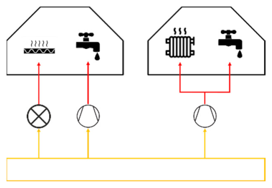 | 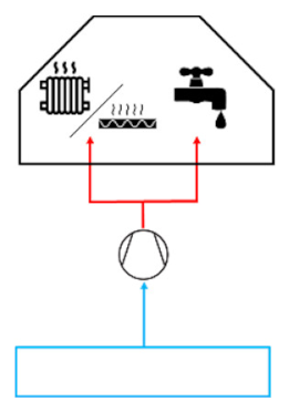 |
| Parameters | ||
| Supply temperature of the DHN | 45 °C | 10 °C |
| Number of users (buildings connected) | 69 | 69 |
| Local HP for SH | 49 | 69 |
| Local HP to boost DWH | 20 | - |
| Thermal power at the local HE | 1440 kW | - |
| Thermal power at the local HP for SH | 6370 kW | 8300 kW |
| Thermal power at the local HP for boost DWH | 490 kW | - |
| Thermal power at the thermal power station | ||
| Module 1 | 2400 kW | 7600 kW |
| Module 2 | 1200 kW | - |
| Module 3 | 4000 kW | - |
| Total | 7600 kW | 7600 kW |
| Component types | ||
| Module 1 | HP | HE |
| Module 2 | HP | - |
| Module 3 | Oil boiler | - |
| Central heat pump COP @ W10/55 | 4.30 | - |
| System at users’ side | Heat exchangers in case of radiant panels as emitting system in the buildings and local HP devoted only to DHW HP devoted to space heating and DHW in case of radiators as emitting system | Local HP for space heating and DHW supply |
| Volume of the TES at the thermal power station | 360 m3 | - |
| Parameters | LT and ULT DHS |
|---|---|
| Set point temperature for SH | 21 °C |
| Throttling range | 0.5 °C |
| Set point temperature of the TES for the DHW | 60 °C |
| Throttling range of the TES for the DHW | 5 °C |
| Heat pump COP @ W10/W55 | 4.96 |
| KPI Energy | Unit | Base Case | Case 1 | Case 2 | Case 3 |
|---|---|---|---|---|---|
| Thermal energy production | MWh/year | 16,157 | 16,867 | 16,813 | 16,753 |
| Share produced by the HP | MWh/year | 14,472 | 16,107 | 16,076 | 15,997 |
| Share produced by the oil boiler | MWh/year | 1685 | 760 | 737 | 756 |
| Electricity consumption (breakdown reported below) | MWh/year | 7680 | 8353 | 8328 | 8297 |
| KPI Thermal Demand and Losses | Unit | Base Case | Case 1 | Case 2 | Case 3 |
| Thermal energy demand (buildings side) | MWh/year | 17,524 | 18,339 | 18,276 | 18,207 |
| Thermal energy demand (network side) | MWh/year | 15,352 | 16,067 | 16,013 | 15,953 |
| Network losses and other effects due to inertia and management | MWh/year | 805 | 800 | 800 | 800 |
| KPI Electricity | Unit | Base Case | Case 1 | Case 2 | Case 3 |
| Electricity consumption of the thermal power station | MWh/year | 4234 | 4764 | 4752 | 4734 |
| Share consumed by the HP | MWh/year | 4228 | 4760 | 4748 | 4730 |
| Share consumed by the oil boiler | MWh/year | 8 | 4 | 4 | 4 |
| Electricity consumption of the hydraulic pump | MWh/year | 367 | 364 | 364 | 364 |
| Electricity consumption of the users | MWh/year | 3078 | 3224 | 3212 | 3198 |
| Average COP of the central heat pumps | - | 3.423 | 3.384 | 3.386 | 3.382 |
| Average COP of the local heat pumps | - | 5.987 | 5.983 | 5.986 | 5.989 |
| KPI Peak Power | Unit | Base Case | Case 1 | Case 2 | Case 3 |
| Peak thermal production | kW | 6306 | 5520 | 5597 | 5681 |
| Peak thermal demand | kW | 7191 | 6315 | 6433 | 6457 |
| Peak electricity consumption | kW | 2476 | 2337 | 2374 | 2379 |
| KPI Flexibility | Unit | Base Case | Case 1 | Case 2 | Case 3 |
| Flexibility factor | - | 0.715 | 0.796 | 0.820 | 0.827 |
| Load factor | - | 0.496 | 0.579 | 0.580 | 0.577 |
| Difference (Base Case—Case n) | Unit | Base Case | Case 1 | Case 2 | Case 3 |
| Thermal energy production | MWh/year | 0 | −710 | −656 | −597 |
| Thermal energy demand | MWh/year | 0 | −815 | −752 | −682 |
| Electricity consumption | MWh/year | 0 | −673 | −648 | −617 |
| Difference (Base Case—Case n) | Unit | Base Case | Case 1 | Case 2 | Case 3 |
| Peak thermal production | kW | 0 | 786 | 709 | 625 |
| Peak thermal demand | kW | 0 | 875 | 757 | 734 |
| Peak electricity consumption | kW | 0 | 140 | 103 | 97 |
| Percentage Difference [(Base Case—Case n)/(Base Case)] | Unit | Base Case | Case 1 | Case 2 | Case 3 |
| Thermal energy production | % | 0.00 | −4.40 | −4.06 | −3.69 |
| Thermal energy demand | % | 0.00 | −4.65 | −4.29 | −3.89 |
| Electricity consumption | % | 0.00 | −8.76 | −8.44 | −8.03 |
| Percentage Difference [(Base Case—Case n)/(Base Case)] | Unit | Base Case | Case 1 | Case 2 | Case 3 |
| Peak thermal production | % | 0.00 | 12.46 | 11.25 | 9.91 |
| Peak thermal demand | % | 0.00 | 12.18 | 10.53 | 10.21 |
| Peak electricity consumption | % | 0.00 | 5.64 | 4.14 | 3.94 |
| KPI Energy | Unit | Base Case | Case 1 | Case 2 | Case 3 |
|---|---|---|---|---|---|
| Thermal energy production | MWh/year | 14,359 | 15,024 | 14,975 | 14,922 |
| Electricity consumption (breakdown reported below) | MWh/year | 5279 | 5355 | 5336 | 5317 |
| KPI Thermal Demand and Losses | Unit | Base Case | Case 1 | Case 2 | Case 3 |
| Thermal energy demand (buildings side) | MWh/year | 17,524 | 18,339 | 18,279 | 18,215 |
| Thermal energy demand (network side) | MWh/year | 14,401 | 15,069 | 15,020 | 14,968 |
| Network losses and other effects due to inertia and management | MWh/year | negligible | negligible | negligible | negligible |
| Thermal demand at the thermal power station (demand + losses) | MWh/year | 14,359 | 15,024 | 14,975 | 14,922 |
| KPI Electricity | Unit | Base Case | Case 1 | Case 2 | Case 3 |
| Electricity consumption of the thermal power station | MWh/year | 72 | 75 | 75 | 75 |
| Electricity consumption of the hydraulic pump | MWh/year | 1652 | 1552 | 1546 | 1540 |
| Electricity consumption of the users | MWh/year | 3556 | 3727 | 3715 | 3703 |
| Average COP of the local heat pumps | - | 4.928 | 4.921 | 4.920 | 4.919 |
| KPI Peak Power | Unit | Base Case | Case 1 | Case 2 | Case 3 |
| Peak thermal production | kW | 5776 | 5068 | 5150 | 5213 |
| Peak thermal demand | kW | 7191 | 6315 | 6441 | 6448 |
| Peak electricity consumption | kW | 2621 | 2184 | 2178 | 2203 |
| KPI Peak Power | Unit | Base Case | Case 1 | Case 2 | Case 3 |
| Peak thermal production | kW | 6306 | 5520 | 5597 | 5681 |
| Peak thermal demand | kW | 7191 | 6315 | 6433 | 6457 |
| Peak electricity consumption | kW | 2476 | 2337 | 2374 | 2379 |
| KPI Flexibility | Unit | Base Case | Case 1 | Case 2 | Case 3 |
| Flexibility factor | - | 0.664 | 0.800 | 0.826 | 0.840 |
| Load factor | - | 0.433 | 0.568 | 0.564 | 0.565 |
| Difference (Base Case—Case n) | Unit | Base Case | Case 1 | Case 2 | Case 3 |
| Thermal energy production | MWh/year | 0 | −665 | −616 | −564 |
| Thermal energy demand | MWh/year | 0 | −815 | −754 | −690 |
| Electricity consumption | MWh/year | 0 | −75 | −56 | −38 |
| Difference (Base Case—Case n) | Unit | Base Case | Case 1 | Case 2 | Case 3 |
| Peak thermal production | kW | 0 | 708 | 627 | 563 |
| Peak thermal demand | kW | 0 | 875 | 750 | 743 |
| Peak electricity consumption | kW | 0 | 437 | 443 | 418 |
| Percentage Difference [(Base Case—Case n)/(Base Case)] | Unit | Base Case | Case 1 | Case 2 | Case 3 |
| Thermal energy production | % | 0.00 | −4.63 | −4.29 | −3.93 |
| Thermal energy demand | % | 0.00 | −4.65 | −4.30 | −3.94 |
| Electricity consumption | % | 0.00 | −1.43 | −1.06 | −0.72 |
| Percentage Difference [(Base Case—Case n)/(Base Case)] | Unit | Base Case | Case 1 | Case 2 | Case 3 |
| Peak thermal production | % | 0.00 | 12.25 | 10.85 | 9.75 |
| Peak thermal demand | % | 0.00 | 12.18 | 10.43 | 10.33 |
| Peak electricity consumption | % | 0.00 | 16.68 | 16.92 | 15.95 |
Publisher’s Note: MDPI stays neutral with regard to jurisdictional claims in published maps and institutional affiliations. |
© 2022 by the authors. Licensee MDPI, Basel, Switzerland. This article is an open access article distributed under the terms and conditions of the Creative Commons Attribution (CC BY) license (https://creativecommons.org/licenses/by/4.0/).
Share and Cite
Toffanin, R.; Caputo, P.; Belliardi, M.; Curti, V. Low and Ultra-Low Temperature District Heating Equipped by Heat Pumps—An Analysis of the Best Operative Conditions for a Swiss Case Study. Energies 2022, 15, 3344. https://doi.org/10.3390/en15093344
Toffanin R, Caputo P, Belliardi M, Curti V. Low and Ultra-Low Temperature District Heating Equipped by Heat Pumps—An Analysis of the Best Operative Conditions for a Swiss Case Study. Energies. 2022; 15(9):3344. https://doi.org/10.3390/en15093344
Chicago/Turabian StyleToffanin, Riccardo, Paola Caputo, Marco Belliardi, and Vinicio Curti. 2022. "Low and Ultra-Low Temperature District Heating Equipped by Heat Pumps—An Analysis of the Best Operative Conditions for a Swiss Case Study" Energies 15, no. 9: 3344. https://doi.org/10.3390/en15093344
APA StyleToffanin, R., Caputo, P., Belliardi, M., & Curti, V. (2022). Low and Ultra-Low Temperature District Heating Equipped by Heat Pumps—An Analysis of the Best Operative Conditions for a Swiss Case Study. Energies, 15(9), 3344. https://doi.org/10.3390/en15093344