Abstract
Effective governance of air pollution requires precise identification of its influencing factors. Most existing studies attempt to identify the socioeconomic factors but lack consideration of multidimensional heterogeneous characteristics. This paper fills this long-ignored research gap by differentiating governance regions with regard to multidimensional heterogeneity characteristics. Decision tree recursive analysis combined with a spatial autoregressive model is used to identify governance factors in China. Empirical results show several interesting findings. First, geographic location, administrative level, economic zones and regional planning are the main heterogeneous features of accurate air pollution governance in Chinese cities. Second, significant influencing factors of air pollution in different delineated regions are identified, especially significant differences between coastal and non-coastal cities. Third, the trends of heterogeneity in urban air governance in China are to some extent consistent with national policies. The approach identifies factors influencing air pollution, thus providing a basis for accurate air pollution governance that has wider applicability.
1. Introduction
Air pollution has become an increasingly prominent environmental issue with industrialization and urbanization in China [1]. Severe and persistent air pollution not only causes substantial economic loss, but also poses serious threats to buildings, biodiversity and human health [2,3,4]. Importantly, air pollution does not have the traditional “territorial” characteristics of environmental governance, but has the characteristic of cross-regional diffusion [5]. Therefore, joint governance and coordinated policies targeting air pollution could contribute to improvements in environmental quality.
The Chinese government has recently paid more attention to air pollution governance. In 2016, it revised and officially implemented the most stringent air pollution law in Chinese history, known as the “Air Pollution Prevention and Control Law”. By introducing the concepts of “joint prevention and control” and “precise air pollution governance”, the government attempted to encourage cities with similar air conditions and urban development to share their air pollution governance experience and conduct joint air pollution enforcement [6].
However, existing joint air pollution governance is constrained by the fact that China has not scientifically and rationally delineated multiple homogeneous joint governance zones. For homogenous joint governance, let us take an example. For a number of cities that are all located in the east and within the same economic circle, and which, when compared, have very similar levels of economic development, industrial structure, etc., then joint air pollution governance in these cities might not only be effective in promoting air pollution, but also save on the cost of policy implementation. This is also in line with Chinese officials looking for collaboration across city and regional boundaries. According to Wu, Xu, and Zhang [5], blind joint efforts can improve air quality to some extent, but cannot achieve long-term air quality stability at a better level. In response to the enforcement of the “Air Pollution Prevention and Control Law”, some cities and city clusters have strengthened regional joint governance and established governance mechanisms. Heavily polluted areas are recognized as the center of a joint air pollution governance area. However, whether this grouping/zoning is reasonable remains an open question. The General Office of the State Council issued the “Guidance on Promoting Joint Prevention and Control of Air Pollution to Improve Regional Air Quality” in 2010. Nine years later, according to the 2019 China Environmental Status Bulletin, 180 out of 337 cities (approximately 53.4%) passed the ambient air quality standards. This outcome indicates that policies of joint air pollution prevention and governance have been proven effective in the short run.
Before discussing grouping, it is necessary to explain the term “heterogeneous”. In this paper, heterogeneity refers to the fact that, when looking at the characteristics of different individuals, the same characteristics are found to manifest themselves in different ways in different individuals; for example, differences in population size, level of economic development, etc., in different countries. These characteristics are called heterogeneous characteristics and the variables used to represent the heterogeneous characteristics are called heterogeneous variables or partitioning variables.
It is inevitable to consider multiple heterogeneous factors when examining homogeneous cities for grouping with regard to the division of air pollution governance areas. The most common grouping methods in the literature are grouping regression and interaction regression, which are usually used to deal with a single heterogeneous characteristic. However, there are problems associated with these two methods. First, the accuracy of estimation will be reduced due to the reduction of sample size. Second, the estimation lacks a “cross-sectional” synthesis of heterogeneous features. Third, the regression coefficients of different groups are not equal, and it is difficult to check whether they are statistically significant [7].
According to Wooldridge [8], interaction term grouping is used to analyse for the full sample, which improves estimation accuracy. However, this approach does not filter and rank the importance of multiple heterogeneous variables and limits longitudinal analysis of heterogeneous characteristics. Therefore, the multidimensional heterogeneous characteristics must be filtered and ranked according to their importance in the governance of urban air pollution firstly. Then, on the basis of grouping, the key factors influencing air pollution in each group are identified, and targeted measures can then be formulated to achieve “common but differentiated” air pollution governance.
Some modern research tools can be well applied to the analysis of air pollution control issues [9]. Machine learning has been widely adopted to estimate heterogeneity using treatment effects [10,11,12]. For example, Athey and Imbens [13] propose a recursive partitioning method for estimating heterogeneous treatment effects, implementing partitioning, and examining treatment effects across partitioned samples. In order to accurately test treatment effects, they use a tree approach that avoids endogeneity bias that arises from using the same sample. This approach is advantageous in differentiating and estimating the effects of heterogeneity.
However, as the available sample size grows, model uncertainty arises from covariate heterogeneity [10]. To identify the effects of covariate heterogeneity, Zeileis, Hothorn, and Hornik [14] propose a recursive analysis method that allows for the better embedding of regression models applying maximum likelihood. Additionally, spatial dependence also plays an important role in examining urban air pollution in China [15,16,17,18,19]. This implies that a simple application of the above-mentioned model, analyzed under the assumption of spatial homogeneity and spatial independence, ignores spatial heterogeneity and would inevitably lead to biased estimates [20,21]. Therefore, the present paper adopts a decision tree recursive analysis approach based on spatial autoregressive models, drawing on the idea of Athey and Imbens [13] to partition the sample using multivariate heterogeneity. Furthermore, recursive analysis [14] is used to identify the impacts of variable heterogeneity due to model uncertainty.
Numerous studies have identified factors that affect air pollution, for example, meteorological factors [22,23]; emission factors; population density [24]; economic growth [25]; industrial structure [26,27], and other socioeconomic factors [28,29,30]. Air pollution is influenced to some extent by meteorological and emission factors, but ultimately stems from many problems in the development process such as sloppy development, imbalanced industrial structure, poor energy structure, energy inefficiency and ineffective environmental governance [20]. Therefore, this paper aims to better clarify the socioeconomic factors contributing to air pollution in China. The environmental Kuznets curve (EKC) hypothesis is proposed as the most direct and effective framework to verify the relationship between air pollution levels and economic development [31]. Estimates of the shape of the EKC vary and include an inverted U-shaped [32,33], U-shaped [34], and N-shaped [35] EKC. Methods such as the joint cubic equation model [36] and panel threshold model [37] are used, but the most straightforward approach is to describe the environmental pollution index in a parametric model, with the income index as an independent parameter or variable in the form of a polynomial function for EKC shape analysis [38]. In addition to the level of economic development, the influence of spatial and other socioeconomic factors on air pollution cannot be ignored. For example, Liu, Wang, and Yang [39] found that urban population concentration and industrialization level have a significant contribution to the air quality index (AQI) [40]. The “pollution refuge” hypothesis suggests that foreign direct investment (FDI) worsens environmental quality by shifting highly polluting industries to host countries [41,42]. Li and Mao [43] found that an increase in fuel consumption per unit of road area led to a deterioration in environmental quality. In summary, the level of economic development, industrial structure, FDI, population concentration, and traffic intensity are important factors influencing air pollution.
The main objective of this paper is to fill in the current research gap by answering the question of how best to delineate air pollution governance areas. It contributes to the literature in the following three areas. First, based on decision tree recursive analysis, we combine machine learning and spatial econometrics to examine the factor influencing air pollution in some major cities in China. The multidimensional heterogeneous characteristics of air pollution and its determinants have not yet been addressed in the literature. Second, this research breaks through the limitation of existing studies by using a priori subjective grouping to take into account the effect of heterogeneity. Based on the data-driven heterogeneity of air pollution, we are able to distinguish areas of air pollution joint prevention and governance in cities. Heterogeneity of air pollution characteristics and the effect of influencing factors are examined simultaneously. Third, the Air Pollution Prevention and Control Action Plan and other policies issued by the State Council focus on air pollution governance in economic circles, provincial capital cities, and part of the eastern cities. Empirical evidence reveals that the dynamic evolution of air pollution heterogeneity is to some extent consistent with these policies. These factors make geographic location, administrative level, regional planning, and economic circles a heterogeneous feature of precise air pollution governance. This suggests more precise air pollution governance.
2. Methodology
2.1. Construction of Spatial Autoregressive Model Based on Partitioning Heterogeneity
Considering the spatial dependence of urban air pollution in China [44], we incorporate the spatial lagged term of the dependent variable into the model, assuming that the vector β can vary across urban subdivisions formed by recursive partitioning. Constructing spatial autoregressive equations based on partitioning heterogeneity:
where i represents the i-th prefecture-level cities (i = 1, 2, 3,..., 283); yi is the mean AQI of the i-th city; yi is the mean AQI of its neighboring city; wi is the vector of spatial weights for the i-th city, and the spatial weight vectors of multiple cities are composed of a spatial weight matrix; ρ is the parameter of the spatial lagged term; xi is a vector of explanatory variables that include the level of economic development, the industrial structure, the level of opening up, the urban transportation infrastructure and population density of the i-th city; βg(i) is the parameter vector of partitioning of the g(i) containing the i-th city, and g(i) is obtained by recursive partitioning of the air pollution heterogeneous variables; and εi is the random error term.
2.2. Recursive Estimation of Unknown Partitioning and Spatial Lag Coefficients
When faced with the need to identify an unknown partition and estimate the model coefficients simultaneously, direct use of existing estimation methods cannot solve these problems. To this end, we draw on the iterative idea proposed by Sela and Simonoff [45] to estimate the spatial lag coefficients of a spatial autoregressive model based on partitioning heterogeneity. Specifically, the iterative estimation process is mainly accomplished as follows. (1) Estimating the spatial lag coefficients when the partition structure is given. (2) Estimating the partition structure when the spatial lag coefficients are given, and the above two processes are completed iteratively. The above iterative process stops when the regression tree no longer changes or when the number of samples is less than the limit value. The detailed process is as follows:
1. Given the groups for all observations , the model in Equation (1) is a standard spatial lag model (with interactions between groups and regressors) and can thus be estimated, for example, by maximum likelihood as discussed from a computational perspective in Bivand and Piras [46]. This yields both and for .
2. Given an estimate of the spatial lag parameter , the dependent variable can be adjusted for the spatial dependence, . Then a standard linear regression tree approach [14] is used to estimate the parameters in Equation (2) and to perform recursive partitioning (as described in the following subsection). This yields an estimate of the group g(i) for each observation .
The described iterative procedure can be initialized in either step: in the first step with all observations in a single group or in the second step without spatial dependence, i.e., with and standard recursive partitioning. In our analysis the results do not depend upon the starting point of the iteration, and we need only one iteration step to reach convergence.
2.3. Estimation of Model-Based Trees
The second step of the estimation algorithm above relies on the estimation of a linear regression tree as discussed in Zeileis, Hothorn, and Hornik [14] that determines the group structure. This iterates between (a) estimating the parameters of Equation (2) in the given (sub)sample by ordinary least squares (OLS), and (b) in case of evidence for non-stable-coefficients splitting the considered sample into two subsamples. For step (b), additional “partitioning” variables are employed with respect to which parameter stability is first assessed and, if any are found, the best split into subsamples is selected by minimizing the residual sum of squares of the partitioned model.
The parameter instability tests considered have first been suggested in the context of time series regressions but can also be applied to other contexts [47,48]. More specifically, the stability of the regression coefficients is tested, using the SupLM test of Andrews [49] for numerical partitioning variables:
where denotes observation of the considered partitioning variable, after ordering according to increasing size denoted by . Furthermore, is the vector of OLS residuals; based on parameter estimation on the considered (sub)sample. is the outer-product-of-gradients (OPG) covariance estimate, employed to normalize the sums of the score vectors .
For categorical partitioning variables, the test statistic is given by:
denoting here with m = 1, ..., M the categories of the partitioning variable , and with the number of observations of in category .
Asymptotic p-values for both tests are computed from the corresponding limiting distributions: supremum of a squared tied-down Bessel process for the SupLM-test [50], and chi-squared with degrees of freedom for the , respectively [51]. Additionally, we apply a Bonferroni-type correction to the p-values to correct for testing along several (and not just a single) partitioning variables. The recursive partitioning procedure stops if no more significant instabilities are detected (at the 5% level) or the subsample becomes too small.
3. Data and Variables
This paper uses the Air Quality Index (AQI) developed by the Chinese government to measure air quality, a dimensionless index that is widely used to provide an important basis for taking measures of air pollution governance. The new version of the AQI (GB3095-2012) was published in most prefectural cities in 2014 and is available at the China General Environmental Monitoring Station and can be downloaded from several official platforms [52]. According to the Chinese standard, the calculation formula is as follows:
where IAQI denotes the individual air quality index; AQI stands for air quality index; IAQI represents the maximum air quality sub-index for the following six pollutants, such as sulfur dioxide (SO2), nitrogen dioxide (NO2), carbon monoxide (CO), ozone (O3), PM10 (particulate matter with a diameter of 10 mm or less), and PM2.5 (particulate matter with a diameter of 2.5 mm or less). n is the number of ambient air pollutants; IAQIp is the air quality sub-index for pollutant p; Cp is the concentration breakpoint that is ≥CL0; and IAQIL0 is the index breakpoint corresponding to CHi. The calculation of Equations (5) and (6) requires referral to Table 1.

Table 1.
Air quality sub-indices and corresponding pollutant concentration limitation intervals.
The above describes the process of calculating AQI, in terms of data sources. The AQI hourly data from 1 January 2015 to 31 December 2017 were extracted from the National Real-time Urban Air Quality Release Platform of the China Environmental Monitoring Center (CNEMC). All other data were obtained from provincial and municipal statistical yearbooks, the China City Statistical Yearbook and the China Urban Construction Statistical Yearbook. There are several reasons for the selection of the starting and ending times of the study. Firstly, AQI is a relatively new way of measuring air quality in China, and the complete annual AQI data of Chinese prefecture-level cities are only available in 2015 and later. Secondly, the “joint prevention and control” mechanism was officially written into the Air Pollution Prevention and Control Law of the People’s Republic of China in 2015. It required input from all sectors of society on the division of the joint prevention and governance areas. Thirdly, statistics from 2018 showed that the targets set for 2017, as proposed in the 2013 State Council’s Action Plan for the Prevention and Control of Air Pollution, i.e., the “Ten Articles of Air”, were fully achieved in 2017. Indeed, 2017 was a year of fruitful achievements of the Action Plan for the Prevention and Control of Air Pollution. To assess the effectiveness of national policies, we use the data period from 2015 to 2017. Some prefecture-level cities were excluded due to a lack of data, and 283 cities were selected in the study.
In this paper, we analyze the heterogeneous characteristics of air pollution. The dependent and independent variables are standardized in order to eliminate the influence of dimension. Table 2 provides the definition of these variables. The selection and relevant literature of those variables can be seen in the Appendix A.
Table 2.
Definitions of variables.
The descriptive statistics have been displayed in Table 3. The mean of AQI is 77.09. The maximum and minimum values for each of the explanatory variables vary considerably, suggesting significant differences in socioeconomic factors between cities. This reflects that there is indeed a need to differentiate air pollution governance according to the heterogeneous characteristics of cities.
Table 3.
Descriptive statistics of dependent and independent variables.
Figure 1 and Figure 2 show the spatial distribution of AQI in 283 cities for the period 2015–2017, indicating that it is initially determined that AQI has strong spatial autocorrelation. Green areas indicate cities with AQI values between 0 and 50, with better air quality, due to better implementation of pollution prevention policies or the city of own natural endowment. It is worth mentioning that some cities in Heilongjiang Province have better air quality. According to the “Heilongjiang Air Quality” app, Heilongjiang Province has eight of the top nine cities in air quality ranking of China. This outcome may largely result from the relevant policy implementations, such as “Heilongjiang Province Ban on Open Burning of Straw” and the “zero” coal-fired small boilers in built-up areas of cities above the prefecture-level, previously issued by the General Office of the Heilongjiang Provincial Party Committee and the General Office of the Heilongjiang Provincial Government. The yellow area indicates cities with AQI values between 51 and 100, with average air quality, and accounts for a relatively large proportion of the cities in most regions of China. The red area indicates cities with AQI values between 101 and 150, with poor air quality, and is mostly concentrated in cities with strong industrial development and high population density. This is intuitive preliminary evidence that industry and population density have a greater impact on air quality.
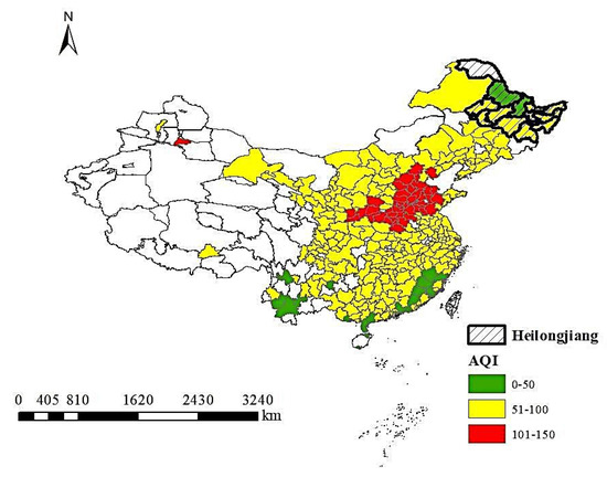
Figure 1.
Spatial distribution of AQI in 283 cities for the period 2015–2017.
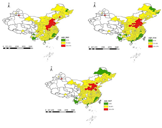
Figure 2.
Spatial distribution of AQI in 283 cities for the period 2015–2017 by year.
4. Results and Discussion
Moran’s I test results show a significant spatial autocorrelation in air pollution. Therefore, we use the decision tree recursive analysis method, and analyze the heterogeneous effects of air pollution in 283 Chinese cities by using the simultaneous testing, and cross-tabulation analysis, of the heterogeneous characteristics of air pollution, incorporating the spatial autoregressive model to estimate the effects of influencing factors on air pollution.
4.1. Parameter Stability Tests and Analysis of Model-Based Trees
Table 4 reports the results of the parametric stability tests of the recursive analysis during the period 2015–2017. According to the principle of recursive partitioning described in Section 2, recursive partitioning stops when no more significant parameter instability is detected or if the number of subsamples is too small. We use the lagsarlmtree program package of R software to automatically complete this series of recursive processes. The results of each of the n iterations in the table represent the formation of the n nodes in Figure 1, which are first determined by the parametric stability test and then displayed in Figure 1. After a variable has been determined to be significant, the next iteration will discard the determination of that variable, i.e., the “NA” situation. Take the results of the 2015 parameter stability test as an example. The Coa and East variables screened in the first two iterations correspond to the Coa and East variables of node 1 and node 2 in Figure 3a, respectively, and their corresponding p-values are also one-to-one. In the third iteration, the variables with significant p values are not screened out, and the subgroup in node 4 is used for the re-test (at which point the Coa and East variables are also determined to be significant). Therefore, the results for NA remain unchanged in the fourth iteration, where again no significant p-values are screened out, and the subgroup in node 5 is used for the re-test (where only the Coa variable is judged to be significant), so that only the parameter corresponding to Coa is NA. The iterations for 2016 and 2017 are carried out in the same way. This has resulted in five, seven and five recursive processes completed during 2015–2017, respectively.
Table 4.
Results of the parametric stability test for the period 2015–2017.
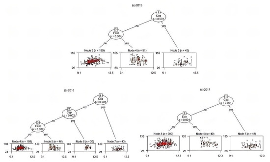
Figure 3.
Regression tree for 2015, 2016 and 2017. Notes: In graph (a) or (c), Nodes 1 and 2 of the decision tree show the filtered partitioning variables, the p-values are from the parametric stability tests, and the red lines of Nodes 3, 4 and 5 show the scatterplot between AQI and LnPgdp in 2015 or 2017. In graph (b), Nodes 1, 2 and 3 of the decision tree show the filtered partitioning variables, and the red lines of Nodes 4, 5, 6 and 7 show the scatterplot between AQI and LnPgdp in 2016.
Five recursive analysis processes were used to obtain the 2015 results. The first regression test showed that East and Coa passed the 5% significance level test, but the p-value of East was higher than the p-value of the partitioning variable Coa during this regression process. Therefore, based on the selection criteria for partitioning variables proposed in Section 3, even if other variables also passed the significance level test, the partitioning variable Coa was selected as the first partitioning variable. In other words, whether or not it is a coastal city is the primary partitioning factor in the recursive analysis processes of 2015. The results of the second regression indicated that the partitioning variable East was the second partitioning variable. All recursive analyses were completed based on the above process, resulting in a decision tree, as shown in Figure 3a. (1) In terms of the heterogeneous influence level, Coa is in the first level as the primary partitioning factor. East is in the second level. (2) Regarding the degree of influence of heterogeneity, the coefficient of the partitioning variable Coa is 53.78, East is 25.14, the degree of influence of heterogeneity shows a decreasing trend. (3) As for the number of subgroups, the 283 cities in China are divided into three subgroups based on the two partitioning variables mentioned above. Node 4 represents 51 non-coastal, eastern cities. Node 5 represents 43 coastal cities and Node 3 represents the rest of 189 non-coastal, non-eastern cities.
Seven recursive analysis processes were used to obtain results for 2016. Three partitioning variables, geographic location, administrative level and economic zone, were screened (Figure 3b). (1) In terms of the heterogeneous influence level, Coa is in the first level as the primary partitioning factor. Cap is in the second level and East is in the third level. (2) Regarding the degree of influence of heterogeneity, the coefficient of the partitioning variable Coa is 48.39, Cap is 26.92 and East is 22.87, showing a decreasing trend. (3) As for the number of subgroups, 283 cities are divided into four subgroups based on the three partitioning variables mentioned above. Node 4 represents 168 non-coastal, non-provincial-capital, non-east cities. Node 5 represents 46 non-coastal, non-provincial-capital, east cities. The number of non-coastal east cities in Node 4 decreased from 51 in 2015 to 46 in 2016. This is because as Cap is added as a partitioning variable in the 2016 screening, the five non-provincial-capital cities were eliminated from Node 4. Node 6 represents 26 non-coastal, provincial capital cities, and Node 7 represents 43 coastal cities.
Five recursive analysis processes were used to obtain results for 2017. Two partitioning variables, geographic location and regional planning, were screened (Figure 3c). (1) In terms of the heterogeneous influence level, Coa is in the first level as the primary partitioning factor. Eco is in the second level. (2) Regarding the degree of influence of heterogeneity, the coefficient of the partitioning variable Coa is 55.93 and Eco is 28.05. (3) As for the number of subgroups, the 283 cities in China are divided into three subgroups. Node 3 represents 200 non-coastal, non-economic circle cities. Node 4 represents 40 non-coastal, economic circle cities, and Node 5 represents 43 coastal cities.
Based on results of Table 4 and Figure 3, the tendency of heterogeneous characteristics of urban air governance in China is to some extent consistent with the orientation of national policies in China (See Table A2). The Air Pollution Prevention and Control Action Plan put forward “the Beijing-Tianjin-Hebei, Yangtze River Delta and Pearl River Delta regions” to complete the construction of regional, provincial and municipal heavy polluted weather monitoring and early warning systems before 2015. Other provinces, sub-provincial cities, and provincial capitals, by the end of 2015, were to complete the construction of regional, provincial and municipal heavy polluted weather monitoring and early warning systems. The sentences “joint prevention and control” appears several times in the document, including key regional air pollution prevention and control in the “Twelfth Five-Year” plan. The partitioning variables for regional planning (Eco) and administrative level (Cap) are important factors for the heterogeneity of urban air pollution during 2015–2017. Because of the great promotion of joint prevention and governance, the economic circle and the radiation effect of the provincial capital cities make coastal (Coa) and eastern (East) cities gradually gathered into the area of joint prevention and governance. Therefore, geographic location and economic zone also become important partitioning factors influencing heterogeneity.
4.2. Estimation Results
Table 5 reports the results of recursive analysis of the factors influencing air pollution for the period 2015–2017 under the inverse distance spatial weight matrix (SWM).
Table 5.
Results of a recursive analysis of air pollution influences for the period 2015–2017.
Results for 2015 show that: (1) For 189 non-coastal, non-eastern cities, population density has a significant positive effect on air pollution. The shift of industries from coastal areas to inland areas has increased the population density in inland areas, and frequent human activities have increased emissions from production and living, thus contributing to air pollution conditions. The estimated slope coefficients of LnPgdp is significantly positive, and the coefficient of LnPgdp2 is significantly negative, revealing an inverted U-shaped relationship between economic growth and air pollution. Chinese inland regions developed rapidly, pursuing economic development at the expense of air pollution. When GDP per capita reached 81,397 RMB (see Table A3), air pollution started to decline. These results are in line with the findings of Liu et al. [54]. (2) For the 51 non-coastal eastern cities, transportation infrastructure has a positive effect on air pollution. In eastern cities, improved transportation infrastructure and financial security resulted in increased air pollution from more vehicles, a result consistent with Li and Mao [43]. In addition, population density has a significantly positive effect on air pollution. The increased share of secondary production improved air quality can be explained by industrial structural changes and investment in more efficient technologies that would enhance the ecological environment [55]. (3) For 43 coastal cities, the coefficient of industrial structure is significantly positive, indicating that an increase in the share of secondary production makes the air quality gradually deteriorate. This is because the coastal area attracts a large number of high emissions enterprises due to its geographical location, and the developed secondary industry contributes to air pollution by emitting large amounts of pollutants, which is in line with Liu et al. [54] and Zhang, Sun, and Wang [56].
The results for 2016 show that: (1) It is further verified that Coa and East are important heterogeneous variables. (2) For 168 non-coastal, non-provincial-capital and non-east cities, and 46 non-coastal, non-provincial-capital and east cities, the significance and magnitude of factors that influence air pollution remained consistent with the results of 2015. (3) For 26 non-coastal and provincial capital cities, only population density passes the 1% significance test. In these cities, human activities largely contributed to worsening air pollution. (4) For 43 coastal cities, the coefficient of LnPgdp is significantly negative, and the coefficient of LnPgdp2 is significantly positive, indicating the EKC curve of coastal cities in 2016 is U-shaped as being a part of the N-shaped curve in the long run. In addition, industrial structure and FDI also passed the 5% significance test. The results of FDI are in line with List and Co [41]. Coastal cities are more open to the outside world and attract more foreign investment than non-coastal cities. Production activities of foreign-funded enterprises caused increased air pollution due to an increase in the level of open up. Industrial development in coastal cities plays an important role in economic development. The rapid growth of secondary industries at the expense of the environment aggravates air pollution.
The results for 2017 show that: (1) For 200 non-coastal and non-economic circle cities, likewise in 2015, we found the inverted U-shaped EKC curve. The number of cities crossing the EKC inflection point continued to increase. However, the number of cities crossing the inverted U-shaped EKC curve was still small (See Table A3), indicating that economic growth in most Chinese cities still largely caused deterioration in air quality. This is more in line with the research findings of the Research Group of the Development Research Center of the State Council [57]—China’s environmental governance is in a state of “partial improvement and overall deterioration”. In the future, under the influence of the “demonstration effect” of inland cities with high economic development, cities may cross the EKC inflection point through the “catch-up effect”. The effect of population density on air pollution was positive. (2) For 40 non-coastal and economic circle cities, population density remained a positive impact on air pollution. (3) For 43 coastal cities, the same as found in 2015 and 2016, the coefficient of Seci remained significantly positive. Different from inland cities, economic development and population density did not pass the significance level test. This is because coastal cities are under environmental protection pressure, and economic development patterns are more focused on the quality of development than in non-coastal cities. The contradiction between the pressure to protect the environment and the need to increase GDP makes economic development insignificant to air pollution. In addition, the intensity of environmental regulation in coastal cities has led to the out-migration of polluting enterprises, as well as the migration of many laborers to inland cities, leading to an insignificant contribution of population density to air pollution in inland cities.
In summary, there are heterogeneous factors for urban air quality, indicating the importance of identifying factors that influence air pollution by first considering the multidimensional heterogeneous characteristics. Specifically, population density is a stable factor influencing air quality in non-coastal cities, and industrial structure is a stable factor influencing air quality in coastal cities. Moreover, improved transportation infrastructure contributes to reducing air pollution in non-coastal eastern cities.
4.3. Robustness Tests
We evaluate the robustness of the results of the above recursive analysis using different cross-period data and alternative SWM (K-neighbor SWM and distance-neighbor SWM) and report results in Table A4, Table A5 and Table A6. We found that the main results of the selection of heterogeneous variables and the analysis of influencing factors are consistent with those when changing the sample period and SWM, which verify the robustness of the main findings. A detailed analysis of robustness is available in the Appendix A.
4.4. Identification of Areas for Precise Governance of Air Pollution
The previous analysis shows that air governance in Chinese cities has produced significant differentiation under the influence of coastal, the provincial capital, the economic circle, and east cities. However, precise air pollution governance should identify the heterogeneous characteristics of air pollution, and at the same time, require the homogeneity of regional governance effectiveness to achieve efficient air pollution reduction. Thus, the results of the recursive analysis in Table 5 are used to identify areas for precise governance of air pollution.
According to two partitioning variables screened in 2015, 283 cities were divided into three urban clusters, with the number of cities being 189, 51 and 43, respectively. Then, according to three partitioning variables screened in 2016, 283 cities were divided into three urban clusters, with the number of cities being 168, 46, 26 and 43. Combining the results of 2015 and 2016, the cities that existed in the same urban cluster changed, and 189 cities originally in the same urban cluster in 2015 were divided into two subgroups with 168 and 21 cities. Meanwhile, 51 cities originally in the same urban cluster were divided into 46 and 5 subgroups, and 43 cities that existed in the same urban cluster remained unchanged during the two years of urban cluster division. Thus, by 2016, cities that existed in the same city cluster were divided into five sub-clusters. Finally, based on two subdivision variables screened in 2017, 283 cities were divided into three city clusters, with the number of cities being 200, 40 and 43, respectively. Combining the results of 2015, 2016 and 2017, the cities that existed in the same city cluster were divided into seven sub-clusters. The number of cities in each sub-cluster was 20, 5, 163, 4, 30, 16 and 43, respectively. In summary, among 283 Chinese cities, seven regions of differentiated air pollution governance can be composed over 2015–2017, as shown in Figure 4.
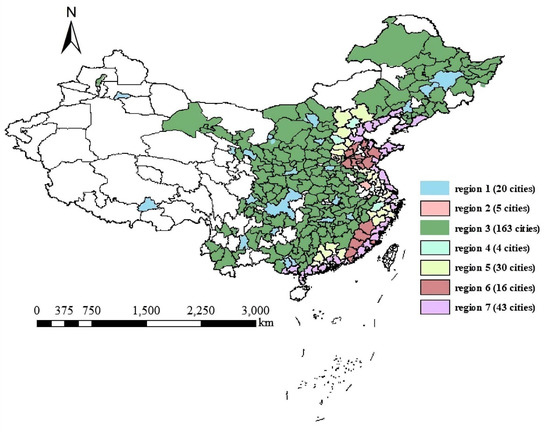
Figure 4.
Differentiated urban air pollution governance area in China.
Further investigation reveals that many cities in the above-mentioned air pollution governance regions are located in the same city cluster officially divided. Many cities that are not members of city clusters are also included in the same control region. It can be seen that Chinese urban air pollution control must break the “fragmented” mode of governance. It is important and necessary to establish a cross-city cluster joint prevention and control governance system to control air pollution accurately and efficiently. This conclusion also supports the study of Liu, Sun, and Chen [18]. In addition, air pollution governance factors have a homogeneous influence across city clusters, the experience of policies and regulations to reduce air pollution can be promoted to each other. It should be noted that the differential air pollution governance across city clusters is not an unconditional integrated joint prevention and control. Rather, localized and precise governance in the seven air pollution governance regions are needed based on the heterogeneous conditions of air pollution.
5. Conclusions and Policy Implications
This paper screens for several heterogeneous characteristics used for regional grouping and identifies the socioeconomic factors that influence air pollution in 283 cities of China from 2015 to 2017 using a combination approach of machine learning and spatial econometrics. Based on heterogeneous characteristics, these cities were divided into seven “common but differentiated” air pollution governance areas. In doing so, this paper resolves the contradiction between global improvements and localized improvements that are insufficient and provides theoretical reference and decision-making reference for the precise and efficient formulation of urban air pollution governance policies in China. The main conclusions are as follows.
(1) Recursive analysis of air pollution shows that geographic location was the first partitioning variable, followed by administrative level heterogeneity (provincial capital or not), economic zone heterogeneity (east or not), and regional planning heterogeneity (economic circle or not). Based on the results of recursive analysis, seven regions of differentiated air pollution governance are identified. After considering spatial spillover of air pollution, seven regions should avoid the disadvantages of territorial governance and carry out regionally differentiated and precise air pollution governance according to the principle of “common but differentiated”.
(2) On the premise of considering multidimensional heterogeneity, economic factors have a differentiated influence on air pollution in different regions. During 2015–2017, increased secondary production share of GDP led to an increase in air pollution in coastal cities. Rising population density also is associated with increased air pollution in non-coastal cities. Transportation infrastructure was also an important factor that exacerbated air pollution in non-coastal east cities by upgrading and building modern infrastructure attracting more vehicle users. In addition, the EKC has been partially validated in China. The number of cities crossing the inverted U-shaped EKC curve continued to increase for three years. However, the number of cities crossing the inverted U-shaped EKC curve was still too small, indicating that economic growth in most Chinese cities largely caused deterioration in air quality.
(3) From the perspective of spatial overflow, the trend of heterogeneous characteristics of urban air pollution in China is highly in line with pollution governance policies issued by the State Council. Heterogeneous partitioning variables filtered by machine learning data-driven filtering maintain a greater degree of consistency with what these policies focus on. Therefore, national policies are scientific and reasonable, and should play a guiding role in urban air pollution governance in China to reduce air pollution.
Our empirical findings support the following suggestions for policy. First, based on Chinese urban air pollution heterogeneity, it is necessary to establish “common but differentiated” air pollution governance regions. Due to different natural geographical conditions and economic development levels of cities, there are differences in the sources and diffusion conditions of air pollution, requiring air pollution governance policies to focus on regional differences and measures of implement refined and differentiated governance. In addition, the external environment and the progress of air pollution governance are in a state of dynamic change. Thus, static pollution governance policies can no longer be adapted to the current stage of pollution governance. Therefore, the governance model should be contracted, refined, and differentiated according to the multidimensional heterogeneity of air pollution characteristics. The development of dynamic air pollution governance policies should keep pace with dynamic changes in pollution status.
Second, machine learning concepts and models, real-time supervision, and timely update of air pollution-related data should be employed when implementing dynamic air pollution governance policies. On the other hand, the government should also increase its investments in education, provide scientific and technological support, and improve the digital intelligent equipment and technology. In summary, in order to effectively improve urban environmental quality, China should focus more on building an intelligent pollution governance toolkit through scientific and technological innovation.
There may exist some potential limitations in this paper. Emissions and meteorology are also important factors regarding air pollution, but the impact of meteorology and emissions has not been analysed in the examination of influencing factors. In addition, for the measurement of air quality, the AQI may be somewhat inconsistent with some readers’ evaluation criteria for air quality, which we will improve in future studies.
Author Contributions
Conceptualization, Y.Y., L.W. and S.H.; formal analysis, Y.Y.; investigation, Y.Y., L.W. and S.H.; data curation, Y.Y. and L.W.; writing—original draft preparation, Y.Y., L.W. and S.H.; writing—review and editing, L.W. and S.H. All authors have read and agreed to the published version of the manuscript.
Funding
This research was funded by the National Office for Philosophy and Social Sciences, grant number: 20FGLB038.
Institutional Review Board Statement
Not applicable.
Informed Consent Statement
Not applicable.
Data Availability Statement
Data are available after kind request to the corresponding author.
Conflicts of Interest
The authors declare no conflict of interest.
Appendix A
Appendix A.1. Measure of Spatial Autocorrelation
Spatial dependence (or autocorrelation) is a fundamental property of all attributes located in space. Moran’s I, Geary’s C, General G, etc., are measures of spatial autocorrelation that indicate whether a variable exhibits significant spatial dependence at a given scale [54,58]; in this case, these measures determine whether an AQI value does so at the city scale. In this paper, we selected the most commonly used Global Moran’s I to measure the spatial autocorrelation of AQI:
where is the number of cities; , is the AQI of a spatial location , ; and denotes the standard deviation of the samples.
Formally, the membership of the observations in the neighborhood set for each location was expressed through a spatial weight matrix (i.e., ). The scope of Global Moran’s I is [−1, 1]. The z-score was used to test the significance of any spatial autocorrelation.
Table A1.
Global Moran I summary.
Table A1.
Global Moran I summary.
| Statistics | Value |
|---|---|
| Moran’ I | 0.317698 |
| expectation index | −0.003546 |
| variance | 0.000049 |
| z score | 46.080503 |
| p value | 0.000000 |
Appendix A.2. Definition of Variables
Appendix A.2.1. Dependent Variable
AQI is a dimensionless index that quantitatively describes air quality conditions. The AQI can be divided into six levels: 0–50, 51–100, 101–150, 151–200, 201–300, and greater than 300. The magnitude of AQI indicates the quality of air. As the value becomes larger, air pollution becomes more serious.
Appendix A.2.2. Independent Variables
(1) Level of economic development (LnPgdp) is measured by the logarithm of gross domestic product (GDP) per capita; (2) Industrial structure (Seci) is measured by the value-added of the secondary industry as a proportion of GDP; (3) Openness to the outside world (FDI) is measured by the ratio of real foreign investment used in the year as a proportion of GDP; (4) Transportation infrastructure (Road) is measured by urban road area per capita with reference to Chen and Chen [59]; (5) Population density (Pop) is measured using the number of population per unit area.
Appendix A.2.3. Partitioning Variables
Spatial, economic and other factors exhibit multi-dimensional heterogeneous characteristics on the results of existing air pollution studies [60,61], which has severely limited the choice of economic policies for precise air pollution governance in China [62].
For different cities, their level of economic development is also different, and their ability to control air pollution varies, which leads to significant differences in the degree of air pollution improvement due to the different levels of economic development in each city, despite the adoption of the same air control policy. Currently, large and medium-sized cities in China are the main regions where severe air pollution outbreaks occur [63], and the current urbanization process in China is still at the stage of increasing air pollution [64,65]. In fact, Chinese current status of air pollution is showing a gradual spread of first-tier cities as the core to neighboring cities, with concentrated and continuous outbreaks in these urban agglomeration regions [66]. For this reason, the heterogeneity of urban scale has also become a predominant issue that has to be considered in the process of rapid urbanization in China.
Su and Zhang [67] paid attention to the heterogeneity of domestic economic factors on the EKC hypothesis. After classifying the provinces according to the heterogeneity of economic development level, the tertiary industry significantly suppresses environmental pollution in areas with high levels of economic development. In contrast, the primary and secondary industries aggravate environmental pollution in areas with low levels of economic growth. Ma and Zhang [68] conducted an in-depth study of provincial air pollution (PM10) from the aspects of the industry and industrial structure heterogeneity. They found that the overall influence of industrial structure on air pollution is not significant. If we consider the heterogeneity of the economic development level, the more developed the economy, the more prominent the influence of industrial structure on air pollution.
The 2013 China Environmental Status Bulletin, published by the Ministry of Environmental Protection (MEP), shows that the air pollution intensity in provincial capital cities is significantly higher than that in other regions. Guo et al. [69] and Bie et al. [70] found significant differences between the sources of PM2.5 contribution and pollution characteristics in provincial capital cities and non-provincial capital cities. Due to their administrative status, provincial capital cities are also unique in terms of policy guidance and public awareness cultivation for air pollution governance [71,72]. This implies that, at the administrative level, the heterogeneity of whether or not they are provincial capital cities needs to be considered.
Along with the rapid advancement of regional development strategies, such as the Western Development and the Belt and Road construction, the economy of Chinese inland regions is entering a stage of rapid development, and the accompanying air pollution is becoming increasingly serious [73,74]. The State Council issued the Action Plan for the Prevention and Control of Air Pollution, which clearly states that the concentration of PM2.5 in the Beijing-Tianjin-Hebei, Yangtze River Delta and Pearl River Delta regions should be reduced by 25%, 20% and 15%, respectively.
Zhang et al. [66] found that Chinese inland areas show a high-high concentration, while Chinese coastal areas show a significant trend of low-low concentration. Leng, Xian, and Du [75] found that FDI in coastal regions is negatively correlated with air pollution based on geographic location heterogeneity divided into coastal and inland areas. Therefore, the geographical location of coastal cities is also a heterogeneous feature to be considered.
Therefore, considering this regional planning heterogeneous feature will make the examination of urban heterogeneity more comprehensive. Regarding existing studies, we select the following economic and spatial factors as partitioning variables of heterogeneity.
(1) Initial level of economic development (LnPgdp0). The natural logarithm of GDP per capita in 2015 was used as a partitioning variable to reveal the role of the Chinese economic development process on urban air pollution. (2) Initial level of industrial structure (Seci0). The share of value-added of secondary industry in GDP in 2015 was used as a partitioning variable to assess the role of the initial level of industrial structure on air pollution. (3) Urban scale heterogeneity (Devp). We classify first-tier, second-tier, and third-tier cities as large and medium-sized cities and other cities as small cities according to the Notice on Adjusting City Size Classification Criteria issued by the State Council. We then selected whether they are large and medium-sized cities as a partitioning variable to evaluate the role of city size heterogeneity on air pollution. (4) Heterogeneity of economic zones (East). Based on the three major economic zone division methods commonly chosen by existing studies, we select whether or not to belong to the eastern part of the city as a partitioning variable to assess the role of economic zone heterogeneity on air pollution. (5) Administrative level heterogeneity (Cap). This paper takes whether or not they are provincial capital cities as a partitioning variable for administrative level heterogeneity. (6) Regional planning heterogeneity (Eco). This paper chooses cities belonging to the Beijing-Tianjin-Hebei, Yangtze River Delta, and Pearl River Delta economic circles as a regional planning heterogeneous partitioning variable. (7) Geographic location heterogeneity (Coa). Whether it is a coastal city or not is chosen as a partitioning variable for the geographical location heterogeneity.
Table A2.
The comparison of results with national policies.
Table A2.
The comparison of results with national policies.
| Year | Screened Heterogeneous Variables | Policy Documents | Details |
|---|---|---|---|
| 2015 | Coa and East | Air Pollution Prevention and Control Action Plan (2013) [76] and the Key regional air pollution prevention and control “Twelfth Five-Year” plan (2012) [77] | The Beijing-Tianjin-Hebei, Yangtze River Delta and Pearl River Delta regions to complete the construction of regional, provincial and municipal heavy polluted weather monitoring and early warning systems before 2015. |
| 2016 | Coa, Cap and East | Air Pollution Prevention and Control Action Plan (2013) [76] | Other provinces, sub-provincial cities, provincial capitals complete the completion of regional, provincial and municipal heavy polluted weather monitoring and early warning system construction by the end of 2015. |
| 2017 | Coa and Eco | “Thirteenth Five-Year Plan” Comprehensive Work Plan for Energy Conservation and Emission Reduction (2016) [78] | Promote total coal consumption control in Beijing, Tianjin, Hebei and surrounding areas, Yangtze River Delta, Pearl River Delta, Northeast and other key areas, as well as key cities for air pollution prevention and control. |
Table A3.
Statistical table of environmental Kuznets curve (EKC) inflection point situation.
Table A3.
Statistical table of environmental Kuznets curve (EKC) inflection point situation.
| Year | N | Partitioning Variables | Independent Variables | EKC Shape | Inflection Point | Have Crossed | ||||
|---|---|---|---|---|---|---|---|---|---|---|
| Coa | East | Cap | Eco | LnPgdp | LnPgdp2 | |||||
| 2015 | 189 | no | no | — | — | 142.0057 ** | −6.2795 ** | Inverted U | 81,397.5131 | 10 |
| 2016 | 168 | no | no | no | — | 136.5645 ** | −6.2463 ** | Inverted U | 55,915.6733 | 29 |
| 43 | yes | — | — | — | −370.7392 ** | 16.6160 ** | U | 69,989.4643 | 22 | |
| 2017 | 200 | no | — | — | no | 165.5741 *** | −7.5998 *** | Inverted U | 53,814.5954 | 75 |
Notes: N is the number of cities. *** (**) indicates 1% (5%) level of significance. Using the coefficients corresponding to LnPgdp and LnPgdp2 in Table A3, we can roughly derive the inflection point of the estimated EKC curve and determine whether the city had crossed the EKC inflection point. The results are shown above. “Inflection point” indicates GDP per capita (RMB). After the inflection point, GDP per capita will decrease (increase) air pollution for an inverted U-shaped (U-shaped) EKC curve. “Have crossed” indicates the number of cities that have crossed the EKC inflection point.
Appendix A.3. Robustness Tests
The study uses the different data and alternative SWM to check the robustness of the results of the recursive analysis.
Appendix A.3.1. Different Cross-Period Data
The interval data from 2015–2016 were selected for recursive analysis, and the results are shown in Table A4. First, the results are robust in terms of heterogeneous characteristics. Coa is the primary partitioning factor for the presence of heterogeneous influence of urban air pollution and is also at the first level of the heterogeneous characteristics. Likewise, East is selected as heterogeneous characteristics that should be taken into account in the detailed differentiation of air pollution governance. Second, in terms of the effect of the influencing factors, the effect of the remaining cities and the corresponding influencing factors are consistent with 2015. The results of 2015, which is the initial year of the time of the study, are essential parts of the evolution of the zonal characteristics. The fact that this result remains consistent with 2015 indicates that our findings are not significantly affected by changing the sample period, verifying the robustness of our analysis.
Table A4.
Results of a recursive analysis of air pollution influences for the period 2015–2016.
Table A4.
Results of a recursive analysis of air pollution influences for the period 2015–2016.
| Year | Node | N | Partitioning Variables | Independent Variables | ||||||
|---|---|---|---|---|---|---|---|---|---|---|
| Coa | East | LnPgdp | LnPgdp2 | Seci | FDI | Road | Pop | |||
| 2015–2016 | 3 | 189 | no | no | 157.4686 ** | −7.1110 ** | 0.0962 | −0.7913 | −0.0394 | 0.0305 *** |
| (61.74351) | (2.8766) | (0.1052) | (0.5977) | (0.1381) | (0.0039) | |||||
| 4 | 51 | no | yes | 299.7275 * | −14.7221 * | −0.7272 ** | 1.4276 | 1.2650 *** | 0.0360 *** | |
| (172.1520) | (7.9089) | (0.2926) | (1.9475) | (0.2817) | (0.0064) | |||||
| 5 | 43 | yes | — | −329.6359 * | 14.9261 * | 0.5391 ** | 2.6586 * | −0.1319 | −0.0043 | |
| (180.6995) | (8.1413) | (0.2229) | (1.5183) | (0.3050) | (0.0032) | |||||
Notes: N is the number of cities. Estimated slope coefficients and standard errors in brackets. *** (**, *) indicates 1% (5%, 10%) level of significance.
Appendix A.3.2. Alternative SWM
There are human factors in the setting of SWM, so that the results will be affected by different weight matrix settings [79]. To avoid the bias caused by SWM, we use the K-neighbor SWM and distance-neighbor SWM to conduct the robustness check. The spatial autocorrelation test of AQI is conducted under the distance-neighbor SWM and the K-neighbor SWM during 2015–2017. Moran’s I values all pass the 1% significance test, indicating that it is necessary to incorporate the SWM into the model for recursive analysis.
Without considering all cities as proximity, the distance-neighbor SWM is constructed by selecting some cities closer in the distance as proximity cities and assigning values to set distance. In doing so, it weakens the influence of cities further away on the current city and strengthens the radiation effect of the current city on the proximity cities, which is in line with the actual situation. We set the farthest distance between the city and a neighboring city to be “d”, with the geometric center of a city as the center of a circle and “d” as the radius of the circle. A city that is wholly or partially within the circle is considered to be a neighboring city of that city. Here, we take d = 1000 km as an example and report results in Table A6. We find that whether or not one belongs to a coastal city (Coa) is still the primary zoning factor for a primary consideration in developing refined and differentiated measures to control air pollution. We also find that heterogeneity in administrative level (Cap), economic zones (East), and regional planning (Eco) should be given high priority in the process of precise governance of urban air pollution in China. These results show that partitioning variables are the same as when using the inverse distance SWM. In terms of estimation results, population density increased air pollution significantly for non-coastal cities. Industrial structure increased air pollution for coastal cities, except in 2016. This is because, under the distance-neighbor SWM, coastal cities are arranged vertically north–south and have a short horizontal distance east–west; thus, there is a discrepancy when defining neighboring cities compared with the inverse distance SWM. The effects of other influencing factors are consistent with the results under the inverse distance SWM. When we change the value of “d” and continue to repeat this process, the results remain essentially the same.
Table A5.
Results of the recursive analysis of air pollution influences under the distance spatial weight matrix (SWM) (distance = 1000 km) for the period 2015–2017.
Table A5.
Results of the recursive analysis of air pollution influences under the distance spatial weight matrix (SWM) (distance = 1000 km) for the period 2015–2017.
| Year | Node | N | Partitioning Variables | Independent Variables | ||||||||
|---|---|---|---|---|---|---|---|---|---|---|---|---|
| Coa | East | Cap | Eco | LnPgdp | LnPgdp2 | Seci | FDI | Road | Pop | |||
| 2015 | 3 | 189 | no | no | — | — | 197.0675 *** | −8.9476 *** | −0.0394 | −0.9768 | −0.0922 | 0.0374 *** |
| (68.82651) | (3.2136) | (0.1195) | (0.7017) | (0.1534) | (0.0043) | |||||||
| 4 | 51 | no | yes | — | — | 138.7912 | −7.3605 | −0.8967 *** | 0.1978 | 1.5643 *** | 0.0490 *** | |
| (182.9038) | (8.4012) | (0.3226) | (1.9922) | (0.3216) | (0.0079) | |||||||
| 2016 | 4 | 168 | no | no | no | — | 187.3565 *** | −8.6764 *** | 0.1449 | −0.5186 | −0.1704 | 0.0437 *** |
| (67.6716) | (3.1540) | (0.1304) | (0.6171) | (0.1452) | (0.0052) | |||||||
| 5 | 46 | no | yes | no | — | 286.2277 | −14.72060 | 0.9687 ** | 2.4096 | 1.8769 *** | 0.0225 *** | |
| (198.9250) | (9.1248) | (0.4837) | (2.1428) | (0.3216) | (0.0068) | |||||||
| 6 | 26 | no | — | yes | — | 790.8531 | −36.0631 | −0.4539 | −1.0284 | 0.8381 | 0.0264 *** | |
| (838.4983) | (36.9580) | (0.3229) | (1.6279) | (0.5370) | (0.0077) | |||||||
| 7 | 43 | yes | — | — | — | −312.4395 * | 13.9249 * | 0.3135 | 2.6850 * | 0.1793 | −0.0021 | |
| (176.8767) | (7.9676) | (0.2234) | (1.4778) | (0.3087) | (0.0022) | |||||||
| 2017 | 3 | 200 | no | — | — | no | 232.8377 *** | −10.79132 *** | −0.1386 | −0.3536 | 0.0932 | 0.0342 *** |
| (65.4974) | (3.0322) | (0.1055) | (0.4301) | (0.1277) | (0.0037) | |||||||
| 4 | 40 | no | — | — | yes | 118.7733 | −6.5608 | 0.4167 | 1.9221 | 0.0271 | 0.0240 *** | |
| (189.7756) | (8.5890) | (0.3574) | (1.1859) | (0.3549) | (0.0073) | |||||||
| 5 | 43 | yes | — | — | — | −127.5533 | 5.7675 | 0.4500 ** | 0.4315 | −0.0989 | −0.0015 | |
| (185.5439) | (8.3258) | (0.2218) | (1.8102) | (0.3267) | (0.0023) | |||||||
Notes: N is the number of cities. Estimated slope coefficients and standard errors in brackets. *** (**, *) indicates 1% (5%, 10%) level of significance. The total number of cities in the table for the 2015 division is not 283 because 43 cities, for which the results are not significant, are not included in this table.
For the K-neighbor SWM, we set the number of neighboring cities of a city as “K”. Taking the nearest K cities as neighboring cities, the weight of each neighboring city is 1/K. Here, we take K = 4 as an example, and the results are shown in Table A6. The number of neighboring cities is “n”, and the weight of each neighboring city is 1/n. The results of the recursive analysis under the K-neighbor SWM are consistent with the inverse distance SWM. For example, three partitioning variables of geographic location (Coa), administrative level (Cap) and economic zone (East) remain to be selected. For coastal cities, industrial structure is an important factor that influences air pollution. The results pass the 10% significance test for three consecutive years except for the non-coastal provincial-capitals cities in 2015. The air quality is worse as the proportion of secondary industry increases. Probably, it is because the actual interactions are different among non-coastal provincial-capitals cities due to the long distance between these cities, and setting the weights of all these cities to the same 1/K using the K-neighbor SWM would have a relatively large error. In contrast, for non-coastal cities, population density is an important factor influencing air pollution, passing the 5% significance test for three consecutive years. Air pollution is more severe as the population density increases. The effects of other influencing factors are consistent with the results under the inverse distance SWM. When we change the value of “K” and repeat this process, the results remain similar.
Table A6.
Results of a recursive analysis of air pollution influences under the K-neighbor SWM (K = 4) for the period 2015–2017.
Table A6.
Results of a recursive analysis of air pollution influences under the K-neighbor SWM (K = 4) for the period 2015–2017.
| Year | Node | N | Partitioning Variables | Independent Variables | |||||||
|---|---|---|---|---|---|---|---|---|---|---|---|
| Coa | East | Cap | LnPgdp | LnPgdp2 | Seci | FDI | Road | Pop | |||
| 2015 | 4 | 168 | no | no | no | 75.5717 | −3.3421 | 0.0283 | −0.5984 | −0.1295 | 0.0127 *** |
| (46.7392) | (2.1887) | (0.0931) | (0.4775) | (0.1046) | (0.0033) | ||||||
| 5 | 46 | no | yes | no | −88.9346 | 3.4919 | 0.7070 ** | −1.3639 | 1.0983 *** | 0.0140 ** | |
| (123.6079) | (5.6700) | (0.3471) | (1.3420) | (0.2442) | (0.0062) | ||||||
| 6 | 26 | no | — | yes | 1332.0215 ** | −59.1695 ** | −0.5241 ** | −0.1260 | −0.1056 | 0.0113 | |
| (575.2805) | (25.5681) | (0.2203) | (1.2549) | (0.3113) | (0.0069) | ||||||
| 7 | 43 | yes | — | — | −67.1926 | 3.0284 | 0.3411 ** | 0.5097 | −0.2439 | 0.0004 | |
| (128.3653) | (5.7881) | (0.1663) | (1.0919) | (0.2201) | (0.0035) | ||||||
| 2016 | 3 | 214 | no | — | no | 126.7353 *** | −5.9787 *** | 0.1711 ** | −0.2615 | 0.0673 | 0.0109 *** |
| (40.8956) | (1.8950) | (0.0795) | (0.3811) | (0.0888) | (0.0022) | ||||||
| 4 | 38 | yes | — | no | −64.4397 | 2.5820 | 0.3397 * | 0.4893 | −0.0182 | 0.0005 | |
| (137.7697) | (6.1912) | (0.1980) | (1.4754) | (0.2269) | (0.0016) | ||||||
| 2017 | 2 | 240 | no | — | — | 144.5509 *** | −6.6821 *** | −0.0406 | −0.1890 | −0.0144 | 0.0113 *** |
| (39.4003) | (1.8161) | (0.0670) | (0.2719) | (0.0795) | (0.0021) | ||||||
| 3 | 43 | yes | — | — | 40.6801 | −1.8465 | 0.4382 ** | −0.3624 | −0.3405 | 8.7523 × 10⁻⁵ | |
| (125.7874) | (5.6445) | (0.1504) | (1.2265) | (0.2213) | (0.0015) | ||||||
Notes: N is the number of cities. Estimated slope coefficients and standard errors in brackets. *** (**, *) indicates 1% (5%, 10%) level of significance. The total number of cities in the table for the 2016 division is not 283 because 31 cities, for which the results are not significant, are not included in this table.
References
- de Leeuw, G.; van der A, R.; Bai, J.H.; Xue, Y.; Varotsos, C.; Li, Z.Q.; Fan, C.; Chen, X.F.; Christodoulakis, I.; Ding, J.Y.; et al. Air Quality over China. Remote Sens. 2021, 13, 3542. [Google Scholar] [CrossRef]
- Varotsos, C.; Tzanis, C.; Cracknell, A. The enhanced deterioration of the cultural heritage monuments due to air pollution. Environ. Sci. Pollut. R 2009, 16, 590–592. [Google Scholar] [CrossRef] [PubMed]
- Wang, W.; Sun, X.; Zhang, M. Does the central environmental inspection effectively improve air pollution? An empirical study of 290 prefecture-level cities in China. J. Environ. Manag. 2021, 286, 112274. [Google Scholar] [CrossRef] [PubMed]
- Wang, X.; Yin, C.; Shao, C. Relationships among haze pollution, commuting behavior and life satisfaction: A quasi-longitudinal analysis. Transp. Res. Part D: Transp. Environ. 2021, 92, 102723. [Google Scholar] [CrossRef]
- Wu, D.; Xu, Y.; Zhang, S. Will joint regional air pollution control be more cost-effective? An empirical study of China’s Beijing-Tianjin-Hebei region. J. Environ. Manag. 2015, 149, 27–36. [Google Scholar] [CrossRef]
- Feng, Y.; Ning, M.; Lei, Y.; Sun, Y.; Liu, W.; Wang, J. Defending blue sky in China: Effectiveness of the ‘Air Pollution Prevention and Control Action Plan’ on air quality improvements from 2013 to 2017. J. Environ. Manag. 2019, 252, 109603. [Google Scholar] [CrossRef]
- Wooldridge, J.M. Econometrics: Panel Data Methods; Cemmap: London, UK, 2009. [Google Scholar]
- Wooldridge, J.M. Introductory Econometrics: A Modern Approach; Cengage Learning: Boston, MA, USA, 2015. [Google Scholar]
- Cracknell, A.P.; Varotsos, C.A. New aspects of global climate-dynamics research and remote sensing. Int. J. Remote Sens. 2011, 32, 579–600. [Google Scholar] [CrossRef]
- Varian, H.R. Big data: New tricks for econometrics. J. Econ. Perspect. 2014, 28, 3–28. [Google Scholar] [CrossRef]
- Mullainathan, S.; Spiess, J. Machine Learning: An Applied Econometric Approach. J. Econ. Perspect. 2017, 31, 87–106. [Google Scholar] [CrossRef]
- Athey, S.; Imbens, G.W. Machine learning methods that economists should know about. Annu. Rev. Econ. 2019, 11, 685–725. [Google Scholar] [CrossRef]
- Athey, S.; Imbens, G. Recursive partitioning for heterogeneous causal effects. Proc. Natl. Acad. Sci. USA 2016, 113, 7353–7360. [Google Scholar] [CrossRef] [PubMed]
- Zeileis, A.; Hothorn, T.; Hornik, K. Model-based recursive partitioning. J. Comput. Gr. Stat. 2008, 17, 492–514. [Google Scholar] [CrossRef]
- Chen, X.; Ye, J. When the wind blows: Spatial spillover effects of urban air pollution in China. J. Environ. Plan. Manag. 2019, 62, 1359–1376. [Google Scholar] [CrossRef]
- Feng, Y.; Cheng, J.; Shen, J.; Sun, H. Spatial effects of air pollution on public health in China. Environ. Resour. Econ. 2019, 73, 229–250. [Google Scholar] [CrossRef]
- Liu, H.J.; Pei, Y.F. Environmental Kuznets Curve Test of Haze Pollution in China. Stat. Res. 2017, 34, 45–54. (In Chinese) [Google Scholar]
- Liu, H.J.; Sun, Y.N.; Chen, M.H. Dynamic correlation and causes of urban haze pollution. China Popul. Res. Environ. 2017, 27, 74–81. (In Chinese) [Google Scholar]
- Zhang, F.; Wang, F.; Yao, S. High-speed rail accessibility and haze pollution in China: A spatial econometrics perspective. Transp. Res. Part D: Transp. Environ. 2021, 94, 102802. [Google Scholar] [CrossRef]
- Shao, S.; Li, X.; Cao, J.; Yang, L. Economic policy choice of haze pollution control in China: Based on the perspective of spatial spillover effect. Econ. Res. 2016, 51, 73–88. [Google Scholar]
- Chen, S.Y.; Wang, J.M. Research on the evaluation and policy path of urban haze governance in China: A case study of the Yangtze River Delta. China Popul. Res. Environ. 2018, 28, 71–80. (In Chinese) [Google Scholar]
- Liu, L.; Talbot, R.; Lan, X. Influence of climate change and meteorological factors on Houston’s air pollution: Ozone a case study. Atmosphere 2015, 6, 623–640. [Google Scholar] [CrossRef]
- Yu, M.; Zhu, Y.; Lin, C.J.; Wang, S.; Xing, J.; Jang, C.; Huang, J.; Huang, J.; Jin, J.; Yu, L. Effects of air pollution control measures on air quality improvement in Guangzhou, China. J. Environ. Manag. 2019, 244, 127–137. [Google Scholar] [CrossRef] [PubMed]
- Nobel, C.E.; McDonald-Buller, E.C.; Kimura, Y.; Lumbley, K.E.; Allen, D.T. Influence of population density and temporal variations in emissions on the air quality benefits of NOx emission trading. Environ. Sci. Technol. 2002, 36, 3465–3473. [Google Scholar] [CrossRef] [PubMed][Green Version]
- Li, Q.; Song, J.; Wang, E.; Hu, H.; Zhang, J.; Wang, Y. Economic growth and pollutant emissions in China: A spatial econometric analysis. Stoch. Environ. Res. Risk A 2014, 28, 429–442. [Google Scholar] [CrossRef]
- Li, K.; Lin, B. The nonlinear impacts of industrial structure on China’s energy intensity. Energy 2014, 69, 258–265. [Google Scholar] [CrossRef]
- Xu, W.; Sun, J.; Liu, Y.; Xiao, Y.; Tian, Y.; Zhao, B.; Zhang, X. Spatiotemporal variation and socioeconomic drivers of air pollution in China during 2005–2016. J. Environ. Manag. 2019, 245, 66–75. [Google Scholar] [CrossRef] [PubMed]
- Ma, X.; Ge, R.; Zhang, L. Research on the relationship between air quality and economy development in major cities of China. Kybernetes. 2014, 43, 1224–1236. [Google Scholar] [CrossRef]
- Yi, M.; Wang, Y.; Sheng, M.; Sharp, B.; Zhang, Y. Effects of heterogeneous technological progress on haze pollution: Evidence from China. Ecol. Econ. 2020, 169, 106533. [Google Scholar] [CrossRef]
- Li, Z.C.; Peng, Y.T. Modeling the effects of vehicle emission taxes on residential location choices of different-income households. Transp. Res. Part D Transp. Environ. 2016, 48, 248–266. [Google Scholar] [CrossRef]
- Park, S.; Lee, Y. Regional model of EKC for air pollution: Evidence from the Republic of Korea. Energy Policy 2011, 39, 5840–5849. [Google Scholar] [CrossRef]
- Lim, J. Economic Growth and Environment: Some Empirical Evidences from South Korea; School of Economics, University of New South Wales: Kensington, Australia, 1998. [Google Scholar]
- Carson, R.T.; Jeon, Y.; McCubbin, D.R. The relationship between air pollution emissions and income: US data. Environ. Dev. Econ. 1997, 2, 433–450. [Google Scholar] [CrossRef]
- Kaufmann, R.K.; Davidsdottir, B.; Garnham, S.; Pauly, P. The determinants of atmospheric SO2 concentrations: Reconsidering the environmental Kuznets curve. Ecol. Econ. 1998, 25, 209–220. [Google Scholar] [CrossRef]
- Fried, B.; Getzner, M. Determinants of CO2 emissions in a small open economy. Ecol. Econ. 2003, 45, 133–148. [Google Scholar] [CrossRef]
- Shen, J. A simultaneous estimation of environmental Kuznets curve: Evidence from China. China Econ. Rev. 2006, 17, 383–394. [Google Scholar] [CrossRef]
- Sirag, A.; Matemilola, B.T.; Law, S.H.; Bany-Ariffin, A.N. Does environmental Kuznets curve hypothesis exist? Evidence from dynamic panel threshold. J. Environ. Econ. Pol. 2018, 7, 145–165. [Google Scholar] [CrossRef]
- Diao, X.D.; Zeng, S.X.; Tam, C.M.; Tam, V.W. EKC analysis for studying economic growth and environmental quality: A case study in China. J. Clean. Prod. 2009, 17, 541–548. [Google Scholar] [CrossRef]
- Liu, J.; Wang, H.W.; Yang, J. Research on the influencing factors of air pollution in China-an analysis based on the dynamic spatial panel model of Chinese cities. J. Hohai Univ. (Phi. Soc. Sci.) 2017, 19, 61–67, 91–92. (In Chinese) [Google Scholar]
- Hao, Y.; Liu, Y.M. The influential factors of urban PM2.5 concentrations in China: A spatial econometric analysis. J. Clean. Prod. 2016, 112, 1443–1453. [Google Scholar] [CrossRef]
- List, J.A.; Co, C.Y. The effects of environmental regulations on foreign direct investment. J. Environ. Econ. Manag. 2000, 40, 1–20. [Google Scholar] [CrossRef]
- Zugravu-Soilita, N. How does foreign direct investment affect pollution? Toward a better understanding of the direct and conditional effects. Environ. Resour. Econ. 2017, 66, 293–338. [Google Scholar] [CrossRef]
- Li, M.; Mao, C. Spatial effect of industrial energy consumption structure and transportation on haze pollution in Beijing-Tianjin-Hebei region. Int. J. Environ. Res. Public Health 2020, 17, 5610. [Google Scholar] [CrossRef]
- Wu, Z.; Zhang, S. Study on the spatial-temporal change characteristics and influence factors of fog and haze pollution based on GAM. Neural Comput. Appl. 2019, 31, 1619–1631. [Google Scholar] [CrossRef]
- Sela, R.J.; Simonoff, J.S. RE-EM trees: A data mining approach for longitudinal and clustered data. Mach. Learn. 2012, 86, 169–207. [Google Scholar] [CrossRef]
- Bivand, R.; Piras, G. Comparing implementations of estimation methods for spatial econometrics. Am. Stat. Assoc. 2015, 63, 1–36. [Google Scholar] [CrossRef]
- Hjort, N.L.; Koning, A. Tests for constancy of model parameters over time. J. Nonparametr. Stat. 2002, 14, 113–132. [Google Scholar] [CrossRef]
- Zeileis, A.; Hothorn, T. A toolbox of permutation tests for structural change. Stat. Pap. 2013, 54, 931–954. [Google Scholar] [CrossRef]
- Andrews, D.W. Tests for parameter instability and structural change with unknown change point. Econom. J. Econom. Soc. 1993, 61, 821–856. [Google Scholar] [CrossRef]
- Hansen, B.E. Approximate asymptotic p values for structuras-change tests. J. Bus. Econ. Stat. 1997, 15, 60–67. [Google Scholar]
- Zeileis, A. A unified approach to structural change tests based on ML scores, F statistics, and OLS residuals. Economet. Rev. 2005, 24, 445–466. [Google Scholar] [CrossRef]
- Qingyue Data. Available online: https://data.epmap.org (accessed on 28 April 2022).
- Announcement on the Publication of the National Environmental Protection Standard “Technical Provisions on Ambient Air Quality Index (AQI) (on Trial)”. Available online: https://www.mee.gov.cn/gkml/hbb/bgg/201203/t20120302_224146.htm (accessed on 28 April 2022).
- Liu, H.; Fang, C.; Zhang, X.; Wang, Z.; Bao, C.; Li, F. The effect of natural and anthropogenic factors on haze pollution in Chinese cities: A spatial econometrics approach. J. Clean. Prod. 2017, 165, 323–333. [Google Scholar] [CrossRef]
- Copeland, B.R.; Taylor, M.S. Trade, growth, and the environment. J. Econ. Lit. 2004, 42, 7–71. [Google Scholar] [CrossRef]
- Zhang, M.; Sun, X.; Wang, W. Study on the effect of environmental regulations and industrial structure on haze pollution in China from the dual perspective of independence and linkage. J. Clean. Prod. 2020, 256, 120748. [Google Scholar] [CrossRef]
- Research Group of the Development, Research Center of the State Council. Phases of change and problems facing Chinese economy. Manag. World 2002, 9, 3–17. (In Chinese) [Google Scholar]
- Getis, A. A history of the concept of spatial autocorrelation: A geographer’s perspective. Geogr. Anal. 2008, 40, 297–309. [Google Scholar] [CrossRef]
- Chen, S.Y.; Chen, D.K. Air pollution, government regulations and high-quality economic development. Econ. Res. 2018, 53, 20–34. [Google Scholar]
- Pinto, J.P.; Lefohn, A.S.; Shadwick, D.S. Spatial variability of PM2.5 in urban areas in the United States. J. Air Waste Manag. 2004, 54, 440–449. [Google Scholar] [CrossRef] [PubMed]
- Austin, E.; Coull, B.A.; Zanobetti, A.; Koutrakis, P. A framework to spatially cluster air pollution monitoring sites in US based on the PM2.5 composition. Environ. Int. 2013, 59, 244–254. [Google Scholar] [CrossRef] [PubMed]
- Wang, S.; Hao, J. Air quality management in China: Issues, challenges, and options. J. Environ. Sci. 2012, 24, 2–13. [Google Scholar] [CrossRef]
- Chan, C.K.; Yao, X. Air pollution in mega cities in China. Atmos. Environ. 2008, 42, 1–42. [Google Scholar] [CrossRef]
- Han, L.; Zhou, W.; Li, W.; Li, L. Impact of urbanization level on urban air quality: A case of fine particles (PM2.5) in Chinese cities. Environ. Pollut. 2014, 194, 163–170. [Google Scholar] [CrossRef]
- Liu, M.; Huang, Y.; Jin, Z.; Ma, Z.; Liu, X.; Zhang, B.; Liu, Y.; Yu, Y.; Wang, J.; Bi, J.; et al. The nexus between urbanization and PM2.5 related mortality in China. Environ. Pollut. 2017, 227, 15–23. [Google Scholar] [CrossRef]
- Zhang, S.L.; Wang, Y.H.; Li, Y.; Zhang, P.F. Analysis of spatial distribution characteristics and influencing factors of haze in China. China Popul. Res. Environ. 2017, 27, 15–22. (In Chinese) [Google Scholar]
- Su, W.H.; Zhang, C.H. A retest of the Chinese EKC on the heterogeneity hypothesis. Stat. Res. 2011, 28, 66–71. (In Chinese) [Google Scholar]
- Ma, L.M.; Zhang, X. Spatial effects of regional air pollution and the influence of industrial structure. China Popul. Res. Environ. 2014, 24, 157–164. (In Chinese) [Google Scholar]
- Guo, M.M.; Jiang, N.; Wang, S.B.; Duan, S.G.; Zhang, R.Q. Zhengzhou city 2014-2017 air pollution characteristics and impact analysis of meteorological conditions. Environ. Sci. 2019, 40, 3856–3867. (In Chinese) [Google Scholar]
- Bie, S.J.; Yang, L.X.; Gao, Y.; Jiang, P.; Li, Y.Y.; Yang, Y.M.; Zhao, T.; Wang, W.X. Characteristics of atmospheric PM2.5 pollution in the background region of Jinan City and its influence on visibility. Environ. Sci. 2019, 40, 3868–3874. (In Chinese) [Google Scholar]
- Li, X.J.; Wang, J. Preliminary analysis of public awareness of climate change in Northeast China cities. China Popul. Res. Environ. 2012, 22, 118–121. (In Chinese) [Google Scholar]
- Guo, Q.; Wang, Y.; Dong, X. Effects of smart city construction on energy saving and CO2 emission reduction: Evidence from China. Appl. Energy 2022, 313, 118879. [Google Scholar] [CrossRef]
- Sun, Y.; Fei, J. Precision governance of haze pollution based on machine learning. Resour. Sci. 2021, 43, 872–885. (In Chinese) [Google Scholar]
- Cai, X.; Che, X.; Zhu, B.; Zhao, J.; Xie, R. Will developing countries become pollution havens for developed countries? An empirical investigation in the Belt and Road. J. Clean. Prod. 2018, 198, 624–632. [Google Scholar] [CrossRef]
- Leng, Y.I.; Xian, G.M.; Du, S.Z. Foreign direct investment and haze pollution: An empirical analysis based on provincial panel data. J. Int. Trade 2015, 12, 74–84. (In Chinese) [Google Scholar]
- The State Council of the People’s Republic of China. Air Pollution Prevention and Control Action Plan. 2013. Available online: http://www.gov.cn/zwgk/2013-09/12/content_2486773.htm (accessed on 9 March 2022).
- The State Council of the People’s Republic of China. Key Regional Air Pollution Prevention and Control “Twelfth Five-Year” Plan. 2012. Available online: http://www.gov.cn/zwgk/2012-12/05/content_2283152.htm (accessed on 9 March 2022).
- The State Council of the People’s Republic of China. “Thirteenth Five-Year Plan” Comprehensive Work Plan for Energy Conservation and Emission Reduction. 2016. Available online: http://www.gov.cn/zhengce/content/2017-01/05/content_5156789.htm (accessed on 9 March 2022).
- Wen, L.; Sharp, B.; Sbai, E. Spatial Effects of Wind Penetration and its Implication for Wind Farm Investment Decisions in New Zealand. The Energy. J. 2020, 41, 47–72. [Google Scholar] [CrossRef]


Publisher’s Note: MDPI stays neutral with regard to jurisdictional claims in published maps and institutional affiliations. |
© 2022 by the authors. Licensee MDPI, Basel, Switzerland. This article is an open access article distributed under the terms and conditions of the Creative Commons Attribution (CC BY) license (https://creativecommons.org/licenses/by/4.0/).