Performance Evaluation of 1.1 MW Grid-Connected Solar Photovoltaic Power Plant in Louisiana

Abstract

In this work, performance analysis and comparison of three photovoltaic technologies are carried out in the Louisiana climate. During the calendar year of 2018, the University of Louisiana at Lafayette constructed and commissioned a 1.1 MW solar photovoltaic power plant for researching solar power in southern Louisiana and for partial energy demand of the university. It was one of the largest solar photovoltaic power plants in Louisiana when constructed and receives an annual solar insolation of 4.88 kWh/m²/d at latitude minus five degrees (25°) tilt. The solar power plant has a total of 4142 modules and incorporates three module technologies. Preliminary performance data from the system level are presented. The evaluation of different technologies is based on final yield, performance ratio, and capacity factor for one year from September 2019 to August 2020. An economic analysis is carried out using levelized cost of energy for the three photovoltaic (PV) technologies. Finally, the results are compared with simulated results of System Advisor Model (SAM) and PVsyst. It was found that copper indium gallium selenide (CIGS) has better performance ratio of 0.79 compared with monocrystalline silicon and polycrystalline silicon, which have performance ratios of 0.77 and 0.73, respectively. The simulation results correlated with the actual performance of the plant.

1. Introduction

In 2018 and 2019, the United States (USA) produced 10.6 GW and 13.3 GW, respectively, from solar photovoltaic (PV) panels. Cumulative operating photovoltaic capacity in the U.S. exceeded 76 GW_DC at the end of 2019, up from just 1 GW at the end of 2009 [1,2]. Among the total capacity of the USA, only 177.56 MW of the installation is from Louisiana at the date of publication. The majority of solar energy research and installations have happened in the southwest part of the USA, such as California and Arizona; however, very few studies have been performed in the southeast part of the United States, which is in a medium solar resource band [3]. It is important for future innovation to understand the viability of solar photovoltaics and how different types of photovoltaic modules perform in Louisiana. Photovoltaic plant performance is influenced by several weather conditions, such as solar irradiance, ambient temperature, wind speed, and rainfall. As a result, outdoor testing of different PV modules is crucial to identify the most suitable PV technologies for best performance in the local environment [4,5].

In order to identify the best performers across PV technologies, the following parameters are recommended by International Electrotechnical Commission (IEC): final PV system yield, reference yield, and performance ratio (PR) [6]. These performance indices allow cross comparison between PV plants of different types that operate under different climatic conditions. The energy yield from the PV array is the most crucial parameter to assess the viability of any installation, and energy yield and performance ratio are used to compare different PV plants at different locations [7]. It is useful to assess both of these during the planning of the power plant and after a few years of operation [8]. Energy yields are also indispensable for calculating the expected cost of electricity generation for different modules, thus allowing the type of module to be selected with the highest yield-to-cost ratio for a specific installation site [9].

Technical performance evaluated using in-field monitoring data is also useful for PV system designers and installers, research, utilities, and end users. They serve as a benchmark of performance for component manufacturers [10]. In this paper, a 1.1 MW solar PV powerplant is evaluated using in-field data and compared with the modelled data using SAM and PVsyst.

2. Background and Literature Review

Performance analysis of PV technology has been carried out all over the world from the module level to utility scale level in different weather conditions. The analysis period varied from one year to seven years. The important literature and their main findings are discussed in this section. A summary of the studies related to the performance analysis of different solar PV plants and their major findings is presented in Table 1.

Some of the major studies at utility scale were performed in India, where a single PV technology was installed and investigated in the powerplant. Few of them are at smaller scale from 100 kW to 1 MW, such as a 190 kW power plant in Khatkar-Kalan, 100 kW and 200 kW powerplants in Rajasthan, and a 1 MW powerplant in Telangana, where the degradation rate is also determined using four different methods along with performance analysis [11,12,13]. These powerplants were studied for one year. Other powerplants greater than 2 MW were also assessed for one year, except the 5 MW powerplant, which was examined for seven years [10,11,14,15,16]. In addition to performance assessment of polycrystalline silicon (poly-Si) modules by calculating final yield, performance ratio, and system efficiency, degradation and economic analyses were also performed [15].

Furthermore, PV technologies are also compared at the utility scale to find the best performing module technology in some studies. In Kuwait, the 11.15 MW solar PV plant was studied to compare two PV technologies: a thin-film installation of 5.5 MW and a polycrystalline silicon installation of 5.6 MW. The comparison between the two PV subsystems revealed no significant difference between the two technologies [17]. Martín-Martínez and colleagues presented a comprehensive study of the performance of six large PV power plants with different mounting topologies such as single axis tracking system, dual axis tracking, and fixed mount systems in Spain. In the study, the energy yield and PR were calculated for every month [18]. Although that study compares the performance of different technologies, they were installed at several locations and commissioned in different time periods.

Individual modules were also tested using the module PR for 15 different solar module technologies at four different locations over the course of one year [19]. Adouane et al. compared eight PV technologies under harsh climate conditions in Kuwait. The results showed that monocrystalline silicon (mono-Si), polycrystalline silicon (poly-Si), and heterojunction (HIT) modules performed better in high irradiance levels, and CIGS module had good performance at low irradiance levels [20]. It is also worth noting that building integrated photovoltaics (BIPV), bifacial modules with different orientations, microgrids, carpark shelters, and rooftop systems were also studied [21,22,23,24,25].

Table 1. Main findings of performance studies.

Reference	Location	Climate Classification	Size	Studied Technology	Main Contribution/Findings
[14]	India	Tropical, savannah	10 MW	poly-Si	The actual performance closely matches with the simulated performance of PVsyst and solar GIS over the study period.
[17]	Kuwait	Arid	11.15 MW	poly-Si and thin film	Comparison between the thin film and poly-Si PV subsystems reveals no significant difference between the two technologies regarding performance ratios (80.0% for thin film and 80.2% for poly-Si)
[21]	Europe	NA	20 modules	bifacial	Use of panels with 92% bifaciality resulted in a higher yield of up to 3% compared to panels with 70% bifaciality
[18]	Spain	NA	Six power plants of different sizes	poly-Si, mono-Si, a-Si	Fixed tilt, single-axis, and dual-axis tracking systems are studied
[20]	Kuwait	Arid desert	16 modules	eight PV technology mono-Si, poly-Si (2 types), HIT, CdTe, CIGS (2 types), a-Si	A-Si and CdTe performed significantly lower than other technologies
[22]	Singapore	Tropical	190 kW	mono-Si, poly-Si, a-Si, CdTe, CIGS	Simulation predictions shows that east façade and panel slope of 30° and 40° are the most suitable location and inclination in Singapore
Current study	Louisiana, USA	Humid, subtropical	1.1 MW	poly-Si, mono-Si, and CIGS	CIGS performs well in these conditions

Table 1. Main findings of performance studies.

Reference	Location	Climate Classification	Size	Studied Technology	Main Contribution/Findings
[14]	India	Tropical, savannah	10 MW	poly-Si	The actual performance closely matches with the simulated performance of PVsyst and solar GIS over the study period.
[17]	Kuwait	Arid	11.15 MW	poly-Si and thin film	Comparison between the thin film and poly-Si PV subsystems reveals no significant difference between the two technologies regarding performance ratios (80.0% for thin film and 80.2% for poly-Si)
[21]	Europe	NA	20 modules	bifacial	Use of panels with 92% bifaciality resulted in a higher yield of up to 3% compared to panels with 70% bifaciality
[18]	Spain	NA	Six power plants of different sizes	poly-Si, mono-Si, a-Si	Fixed tilt, single-axis, and dual-axis tracking systems are studied
[20]	Kuwait	Arid desert	16 modules	eight PV technology mono-Si, poly-Si (2 types), HIT, CdTe, CIGS (2 types), a-Si	A-Si and CdTe performed significantly lower than other technologies
[22]	Singapore	Tropical	190 kW	mono-Si, poly-Si, a-Si, CdTe, CIGS	Simulation predictions shows that east façade and panel slope of 30° and 40° are the most suitable location and inclination in Singapore
Current study	Louisiana, USA	Humid, subtropical	1.1 MW	poly-Si, mono-Si, and CIGS	CIGS performs well in these conditions

Climate, especially temperature, which has a negative correlation with power, plays a huge role for the PV production. Generally, crystalline silicon modules lose power from 0.4% to 0.45% for every 1 °C increase in temperature as compared to thin film modules, where they lose only 0.2% to 0.23% power/°C. There might be few PV modules with better response, but the majority of them in the market have temperature coefficients in the stated range for power. As a result, research conducted under various climatic conditions is also discussed. The project evaluation of six PV technologies at eight identical, 54 kW sites with different climatic regions in Brazil found that thin-film PV modules with a low temperature coefficient of power presented superior performance [26]. A 2.2 kW system in Brazil with semi-arid climate was investigated for the period from June 2013 to May 2014 [27]. Grid connected photovoltaic systems representing temperate weather were explored in Morocco, Malawi, Italy, and Japan [28,29,30,31]. A 6 MW grid connected system consisting of polycrystalline silicon modules in Algeria in a hot desert climate was examined [32]. These studies use energy yield, performance ratio, and system efficiency as the main parameters for the assessment and monitoring of power plant.

After the real-time evaluation of PV technology, it is important to compare the results with the modelled data for finding the accuracy of the models and future installations. PV predictive modelling is performed at the planning stage of the project most of the time [33]. There are a variety of PV simulation software packages that use different power models, databases, irradiance decomposition methods, and many other features. Souza Silva et al. used HOMER, PV*SOL, and PVsyst to model the PV plant located at the University of Campinas in Campinas, Brazil. Their study found that HOMER underpredicted, PV*SOL overpredicted, and PVsyst was the closest to the values measured at the plant. These results led to the recommendation of PVsyst software for large-scale installations [34]. Malvoni et al. compared the long-term performance of a PV system in southern Italy to the simulated performance using System Advisor Model (SAM) and PVsyst. In the study it was noted that SAM required fewer user inputs than PVsyst, but the models only experienced a 0.1% difference in normalized mean average error of energy output [30].

To the best of the authors’ knowledge, very little information is available on comparison of performance of three major PV technologies at the utility scale. Many studies have been conducted to compare the performance of various PV technologies, but most of them are at the module level. The present work aims to fill this gap and provide real-time long-term performance evaluation of a solar PV plant in humid subtropical weather conditions.

Although there are several solar PV powerplants installed in Louisiana, there has been no published study in Louisiana that compares the performance of different PV technologies. In this study, a 1.1 MW power plant in Lafayette, Louisiana, is investigated based on the performance parameters. Based on the methods presented in the literature, we have evaluated and compared the performance of three module technologies from September 2019 to August 2020 using the parameters such as final yield, PR, system efficiency, and capacity factor. The aim of the paper is to identify the module technology that is most viable in Louisiana. The paper makes a site-specific contribution by assisting solar installers and commercial building owners in Louisiana in determining the type of solar technology that should be installed to maximize yield. The paper also delves deeper into analysing the performance of three technologies on clear and cloudy sky conditions. Finally, the performance is compared with simulated values from System Advisor Model (SAM) and PVsyst.

The paper is organized as follows: Section 3 describes the grid connected photovoltaic system location, module and inverter specifications, and weather station description; Section 4 presents the description and definitions of the technical parameters used in the study; Section 5 demonstrates the performance analysis results of the system and the comparison of actual to simulation results, and, finally, Section 6 presents the conclusion and future recommendations of the study.

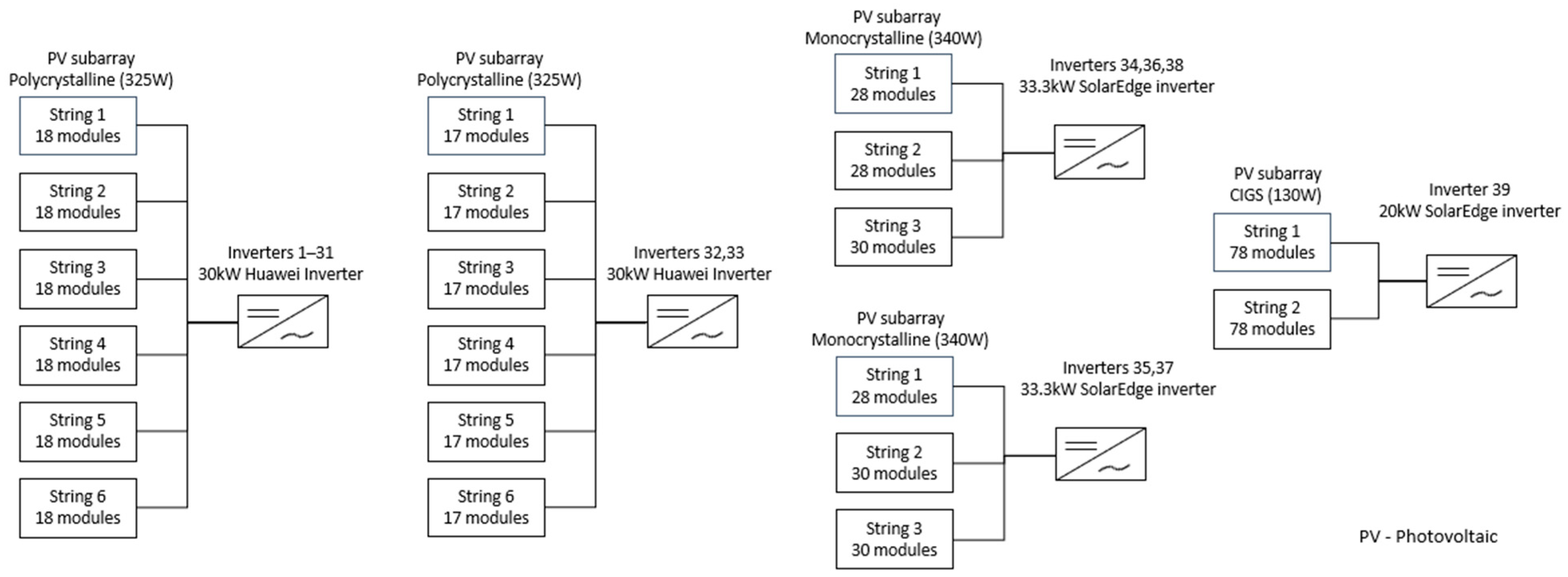
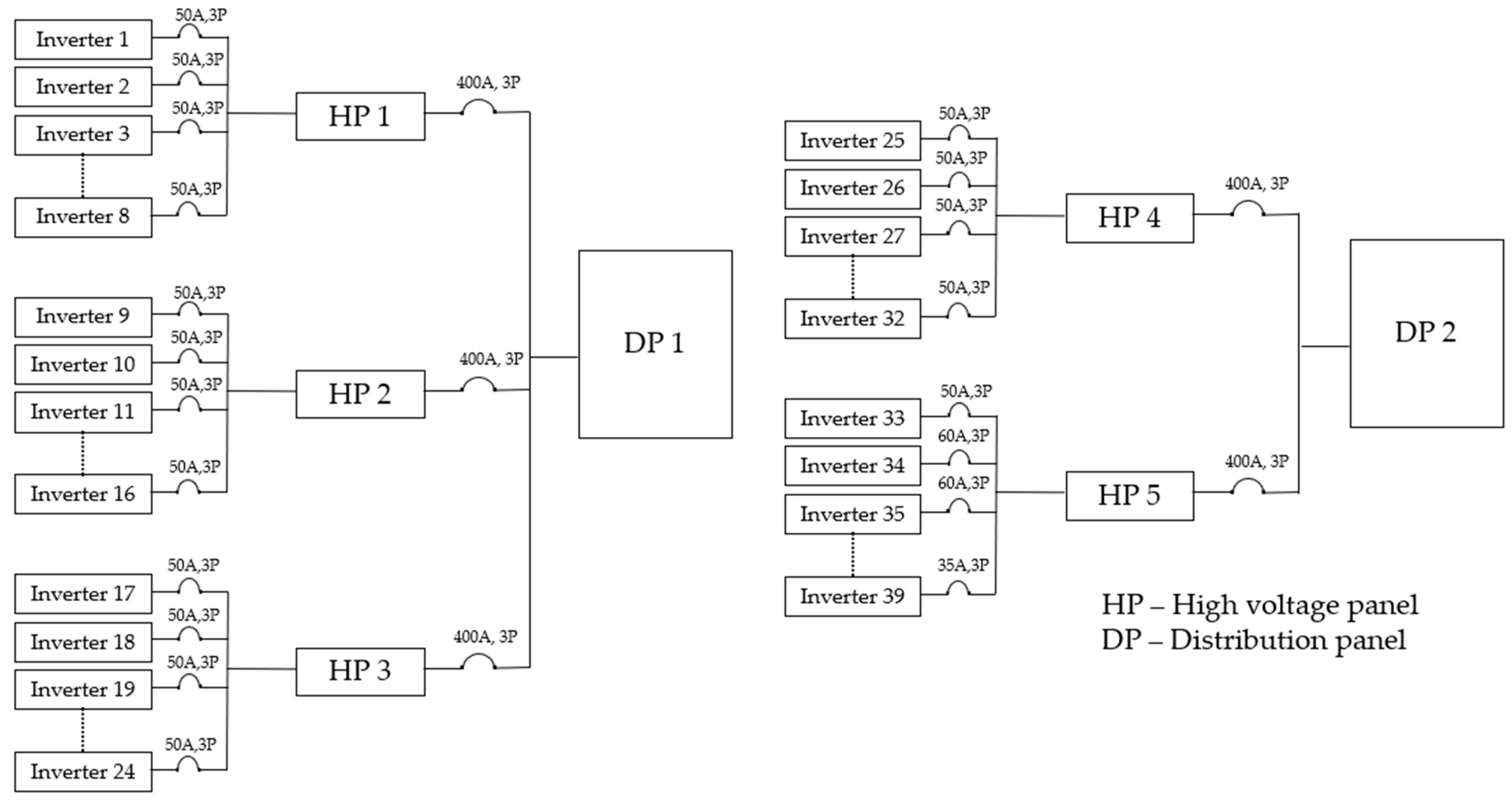
3. Description of the Power Plant

The Louisiana Solar Energy Lab is a 1.1 MW (AC) PV powerplant sited on six acres in the University’s Research Park in Lafayette, Louisiana, where the average solar insolation is 4.88 kWh/m²/d at 25° tilt. Lafayette’s climate is described as temperate (humid subtropical) under the Köppen climate classification. Commissioned in July 2018, it provides 10% of the University’s total peak power demand and supplies 3% of the total energy used.

The Louisiana Solar Energy Lab utilizes three PV technologies: mono-Si, poly-Si, and thin film (CIGS), as well as two inverter types: string inverters and string inverters with power optimizers. Overall, there are 4142 PV modules and 39 inverters. All the modules are fixed and mounted on the ground facing south, installed at a tilt angle of 25°. There are 3552 poly-Si modules with a rated power of 325 W at standard test conditions (STC), 434 mono-Si modules at a rated power of 340 W, and 156 CIGS modules at a rated power of 130 W, as shown in Figure 1. The mono-Si modules and CIGS modules have one power optimizer for every two modules. Detailed specifications are presented in

Table 2. Specifications of PV modules.

Module Manufacturer	Peimar	Seraphim Solar	Stion
Model	SG325P	SRP-340-6MA	STO-130
Framed/frameless	Framed	Framed	Frameless
Technology	Poly-Si	Mono-Si	CIGS * (thin film)
Max power output (Pmax)	325	340	130
Max voltage (Vmp)	36.3	37.7	57
Max current (Imp)	9.03	9.02	2.28
Open circuit voltage (Voc)	44.6	46.6	76.7
Short circuit current (Isc)	9.74	9.32	2.6
Rated efficiency (%)	16.74	17.52	12
Temperature coefficient for power (%/°C)	−0.43%	−0.40%	−0.26%
Temperature coefficient for voltage (%/°C)	−0.32%	−0.32%	−0.24%
Temperature coefficient for current (%/°C)	0.047%	0.05%	0.004%

* CIGS = copper indium gallium selenide.

.

There are 33 string inverters of 30 kW each that are connected to the poly-Si array, five inverters of 33.3 kW each are connected to the mono-Si array, and one inverter with 20 kW capacity is connected to the CIGS array, as shown in Figure 2. All inverters operate at 480 Volts AC. Power optimizers installed on every two modules for mono-Si array and the CIGS array helps to keep them performing at their maximum power point.

AC power from the 39 inverters is combined in five high voltage panels (HP). Each 35 A, 50 A, or 60 A breaker in the HP panels can trip one inverter at a time, as shown in Figure 3. Two distribution panels (DP) combine the power from the five high voltage panels, and each 400 A DP breaker can trip eight inverters at a time for maintenance. The energy passes through 11 kV/400–230 V/1000 kVA transformer. The power from the transformer goes through 11.2 kV lines and reaches the Reinhardt substation for supplying the power to the university.

The weather station containing three Kipp & Zonen pyranometers (one shaded) and one pyrheliometer measures global horizontal irradiation (GHI), plane of array (POA) solar irradiation, direct normal irradiation (DNI), and diffuse horizontal irradiation (DHI). The weather station also measures back-of-module and ambient temperature, wind speed, humidity, air pressure, and precipitation.

4. Methodology

There are many performance parameters developed by the International Energy Agency (IEA) for analyzing the performance of the solar PV grid interconnected system, and the parameters used in this study based on the literature and available data are final yield, performance ratio, system efficiency, and capacity factor.

4.1. Final Yield

Final yield, Y_F, is defined as the total AC energy generated by the PV system for a defined period (i.e., day, month, or year) divided by the peak power of the installed PV array at STC of 1000 W/m² solar irradiance and 25 °C cell temperature. It represents the number of hours that the PV array would need to operate at its rated power to provide the same energy. The Y_F normalizes the energy produced with respect to the system size [6].

$${\mathrm{Y}}_{\mathrm{F}}=\frac{{\mathrm{E}}_{\mathrm{A}\mathrm{C}}}{{\mathrm{P}}_{\mathrm{P}\mathrm{V},\mathrm{R}\mathrm{a}\mathrm{t}\mathrm{e}\mathrm{d}}}$$

(1)

The AC energy, E_AC, can be daily, monthly, or yearly AC energy depending on the time period for which the final yield needs to be calculated, and it can be defined as:

$${\mathrm{E}}_{(\mathrm{AC},\mathrm{d})}={\sum }_{\mathrm{t}=1}^{24}{\mathrm{E}}_{(\mathrm{AC},\mathrm{t})}; {\mathrm{E}}_{(\mathrm{AC},\mathrm{m})}={\sum }_{\mathrm{t}=1}^{\mathrm{N}}{\mathrm{E}}_{(\mathrm{AC},\mathrm{d})}$$

(2)

where E_(AC,d) is the total energy generated in a day, E_(AC,m) is the total energy generated in a month, N is the number of days in the month, and P_PV,Rated is the rated power of the system.

4.2. Reference Yield

Reference yield is the ratio of total plane of array irradiance, H_POA, to the reference irradiance G₀. It represents the obtainable energy under ideal conditions. If G₀ equals 1 kW/m², then the reference yield is the number of peak sun hours, which will be numerically the same as the solar insolation in units of kWh/m². The reference yield defines the solar radiation resource for the PV system and is a function of the location, orientation of the PV array, and month-to-month and year-to-year weather variability [6,14].

$${\mathrm{Y}}_{\mathrm{R}}=\frac{{\mathrm{H}}_{\mathrm{P}\mathrm{O}\mathrm{A}}\mathrm{k}\mathrm{W}\mathrm{h}/{\mathrm{m}}^2}{{\mathrm{G}}_0\mathrm{k}\mathrm{W}/{\mathrm{m}}^2}$$

(3)

4.3. Performance Ratio

The PR is the ratio of final yield to the reference yield. The PR can be defined as comparison of plant output with the output of the plant could have achieved by considering irradiation, panel temperature, availability of grid, size of the aperture area, nominal power output, and temperature correction values [15].

$$\mathrm{PR}=\frac{{\mathrm{Y}}_{\mathrm{F}}}{{\mathrm{Y}}_{\mathrm{R}}}$$

(4)

4.4. Capacity Factor

The capacity factor is a means used to present the energy delivered by an electric power generating system. If the system delivers full rated power continuously, its C_f would be unity. The capacity factor of a solar PV installation is defined as the ratio of the final energy produced by the installation over a given period to the energy output that would have been generated if the system were operated at full capacity for the entire period [35]. For example, the annual capacity factor or capacity utilization factor is given as:

$$\mathrm{CUF} \mathrm{or} \mathrm{Cf}=\frac{{\mathrm{E}}_{\mathrm{A}\mathrm{C}}}{\left({\mathrm{P}}_{\mathrm{P}\mathrm{V}-\mathrm{r}\mathrm{a}\mathrm{t}\mathrm{e}\mathrm{d}}\ast {\mathrm{A}}_{\mathrm{h}}\right)}$$

(5)

where A_h is the total expected number of hours of operation in a given period, which is commonly taken as a year (a regular year consists of 365 days), A_h is the 8760 h, E_AC (kWh) is the total annual energy generated, and P_PV,Rated is the rated power of the system.

4.5. System Efficiency

System efficiency describes the amount of incident radiation flux that is converted to electricity, and it is one of the main indices to determine the overall performance of photovoltaic technologies [36].

$$\mathrm{System} \mathrm{efficiency} {\mathsf{\eta }}_{\mathrm{PV}}=\frac{\mathrm{A}\mathrm{C} \mathrm{E}\mathrm{n}\mathrm{e}\mathrm{r}\mathrm{g}\mathrm{y} \mathrm{g}\mathrm{e}\mathrm{n}\mathrm{e}\mathrm{r}\mathrm{a}\mathrm{t}\mathrm{e}\mathrm{d} \left(\mathrm{k}\mathrm{W}\mathrm{h}\right)}{{\mathrm{H}}_{\mathrm{P}\mathrm{O}\mathrm{A}}\ast {\mathrm{A}}_{\mathrm{s}}}$$

(6)

where H_POA is the total plane of array irradiance, and A_s is the array surface area.

4.6. Levelized Cost of Energy

The levelized cost of electricity, also called the levelized cost of energy, is used as a benchmark that evaluates the cost-effectiveness of different technologies. It can be described as the total life cycle cost over the overall lifetime energy [16,35,37].

$$\mathrm{LCOE}=\frac{\mathrm{T}\mathrm{o}\mathrm{t}\mathrm{a}\mathrm{l} \mathrm{L}\mathrm{i}\mathrm{f}\mathrm{e}\mathrm{c}\mathrm{y}\mathrm{c}\mathrm{l}\mathrm{e} \mathrm{c}\mathrm{o}\mathrm{s}\mathrm{t}}{\mathrm{T}\mathrm{o}\mathrm{t}\mathrm{a}\mathrm{l} \mathrm{E}\mathrm{n}\mathrm{e}\mathrm{r}\mathrm{g}\mathrm{y} \mathrm{g}\mathrm{e}\mathrm{n}\mathrm{e}\mathrm{r}\mathrm{a}\mathrm{t}\mathrm{e}\mathrm{d} \mathrm{i}\mathrm{t}\mathrm{s} \mathrm{l}\mathrm{i}\mathrm{f}\mathrm{e}\mathrm{t}\mathrm{i}\mathrm{m}\mathrm{e}}$$

(7)

$$\mathrm{LCOE}=\frac{{{\displaystyle \sum }}_0^{\mathrm{N}}\frac{\mathrm{I}+\mathrm{O}\&{\mathrm{M}}_{\mathrm{n}}}{{(1+\mathrm{dr})}^{\mathrm{n}}}}{{{\displaystyle \sum }}_0^{\mathrm{N}}\frac{{\mathrm{S}}_{\mathrm{t}}{(1-\mathrm{D}\mathrm{r})}^{\mathrm{n}}}{{(1+\mathrm{dr})}^{\mathrm{n}}}} \$/\mathrm{kWh}$$

(8)

where dr is the discount rate, Dr is the degradation rate, I is the initial investment, O&M is the operation and maintenance cost, N is the lifetime of the project, n is the corresponding year, and S_t is the annual output energy during first year of operation.

4.7. Simulation Using SAM and PVsyst

The validation and the comparison of the performance indices are done using two widely used software packages, PVsyst and System Advisor Model (SAM). PVsyst is a software commonly used by renewable energy professionals to perform technical analyses on different types of PV systems such as grid-connected, stand alone, and battery based [38]. SAM has a more sophisticated performance and financial model than PVsyst and is aimed at a broader audience. It allows for the simulation of multiple renewable technologies, whereas PVsyst is only capable of simulating PV systems.

SAM and PVsyst software contain module, inverter, and weather databases that allow for ease of access to these parameters. The weather data from Solargis are used as inputs for two software in this study. To evaluate the differences between the measured and expected performance from the SAM and PVsyst models, three statistical metrics are utilized. The normalized mean bias error (NMBE) indicates whether the model over or under estimates; the normalized mean absolute error (NMAE) gives the magnitude of error, and the regression coefficient R² defines the relationship between the estimated and measured data using a linear model [30]. They are defined as follows:

$$\begin{array}{c}\mathrm{Normalized} \mathrm{Mean} \mathrm{Bias} \mathrm{Error}\\ \left(\mathrm{NMBE}\right)\end{array}=\frac{{\mathrm{Estimated}}_{\mathrm{i}}-{\mathrm{Measured}}_{\mathrm{i}}}{{\mathrm{Max}(\mathrm{Measured}}_{\mathrm{i}})}\ast 100\%$$

(9)

$$\begin{array}{c}\mathrm{Normalized} \mathrm{Mean} \mathrm{Absolute} \mathrm{Error}\\ \left(\mathrm{NMAE}\right)\end{array}=\left|\frac{{\mathrm{Estimated}}_{\mathrm{i}}-{\mathrm{Measured}}_{\mathrm{i}}}{{\mathrm{Max}(\mathrm{Measured}}_{\mathrm{i}})}\right|\ast 100\%$$

(10)

$${\mathrm{R}}^2=\frac{{{\displaystyle \sum }}_{\mathrm{i}}{\left[\right({\mathrm{Measured}}_{\mathrm{i}}-\overline{\mathrm{M}}\left)\right({\mathrm{Estimated}}_{\mathrm{i}}-\overline{\mathrm{E}}\left)\right]}^2}{{{\displaystyle \sum }}_{\mathrm{i}}{({\mathrm{Measured}}_{\mathrm{i}}-\overline{\mathrm{M}})}^2\ast {({\mathrm{Estimated}}_{\mathrm{i}}-\overline{\mathrm{E}})}^2}$$

(11)

where i represents the month, $\overline{\mathrm{M}}$ represents the monthly average of the measured values, and $\overline{\mathrm{E}}$ represents the monthly average of the estimated values.

5. Results and Discussion

Using the above methodology, performance parameters are determined for the three technologies from September 2019 to August 2020, and the results are shown. The average monthly ambient temperature, direct normal insolation (DNI), diffuse horizontal insolation (DHI), and plane of array (POA) insolation are shown in Figure 4. Data for DHI and DNI are not available for three months from September 2019 to November 2019. The lowest temperature of 14.39 °C is recorded in January and highest of 29.91 °C is recorded in August. Similarly, the lowest and highest daily plane of array insolation is noticed in January (3.49 kWh/m²) and September (5.92 kWh/m²). The lowest amount of diffused insolation (1.03 kWh/m²) is observed in December. The coldest months are from December to February when the insolation and temperature are both low.

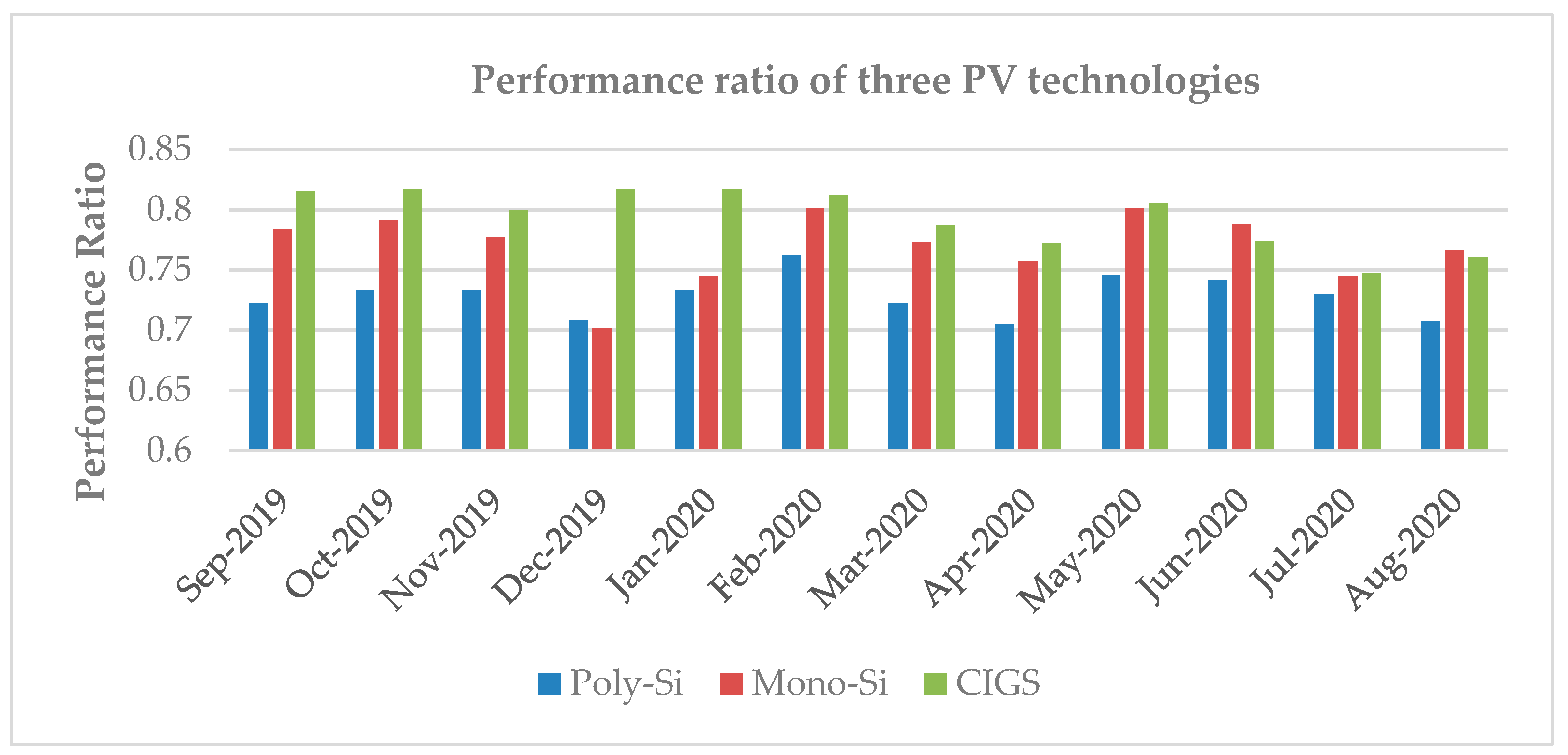
5.1. Final Yield and Performance Ratio

Final yield was calculated for each inverter using AC energy generated from September 2019 to August 2020. Inverters that were down for maintenance were excluded. The average annual final yield for the poly-Si array is 1279 kWh/kW; for the mono-Si array, it is 1356 kWh/kW; and for the CIGS, it is 1392 kWh/kW. The CIGS array has higher final yield compared with the other two technologies.

The PR was also compared for the period from September 2019 to August 2020. The CIGS has a better PR than the other two technologies for most of the time, as shown in the Figure 5. The PR is at its highest for the poly-Si and mono-Si in February, having values of 0.76 and 0.80, respectively, and is at its lowest during month of December. The CIGS array has an average PR of 0.79, whereas the poly-Si and mono-Si arrays have an average PR of 0.73 and 0.77, respectively.

In contrast, the similar study in Kuwait revealed that crystalline silicon modules had better PR than CIGS and it was because of high temperature coefficient of −0.5%/°C and low efficiency of 7.87% for the CIGS modules used in that study [20]. However, for our current study, CIGS has a lower temperature coefficient of −0.26%/°C, hence it performs better than its counterparts.

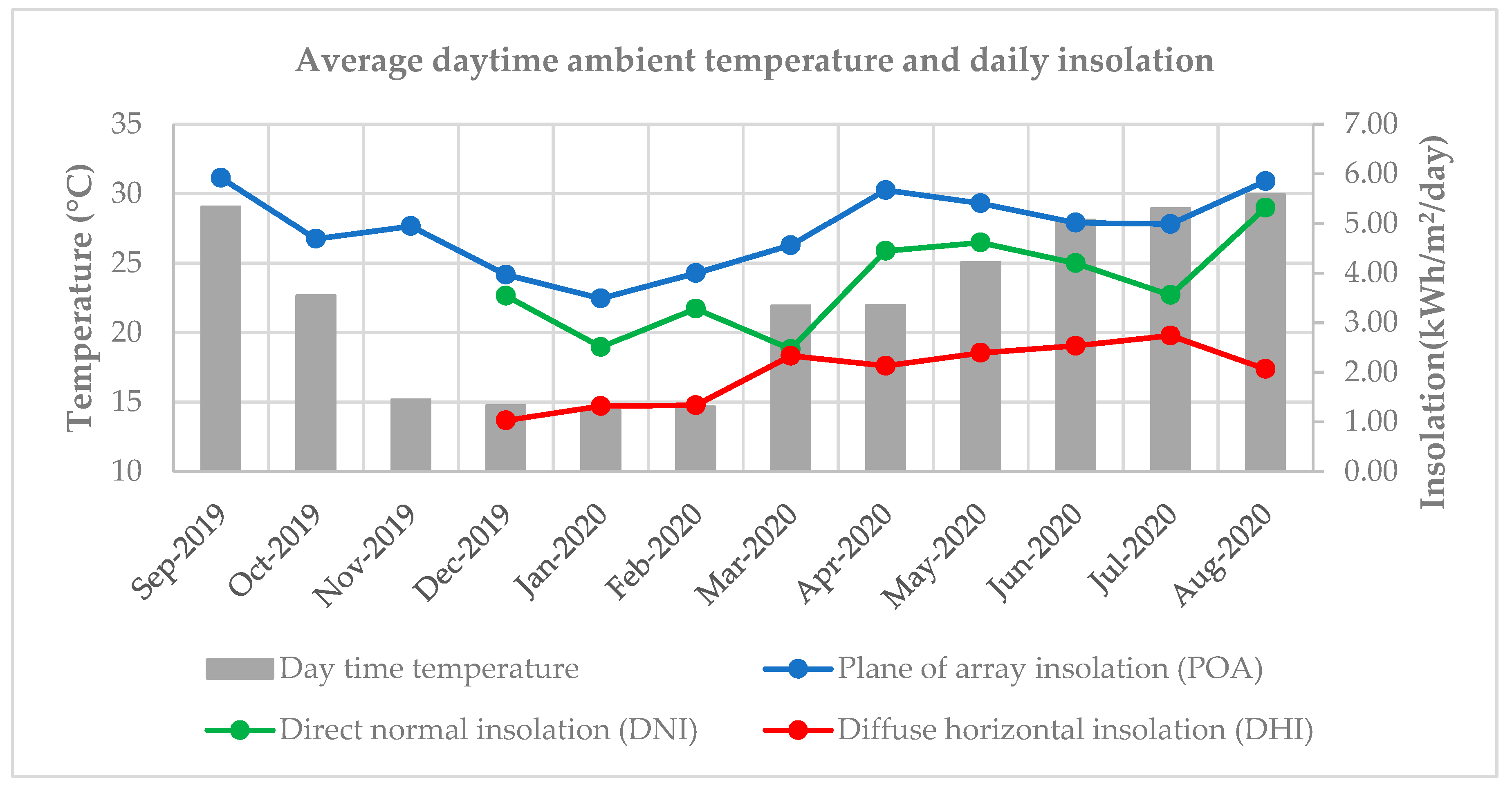
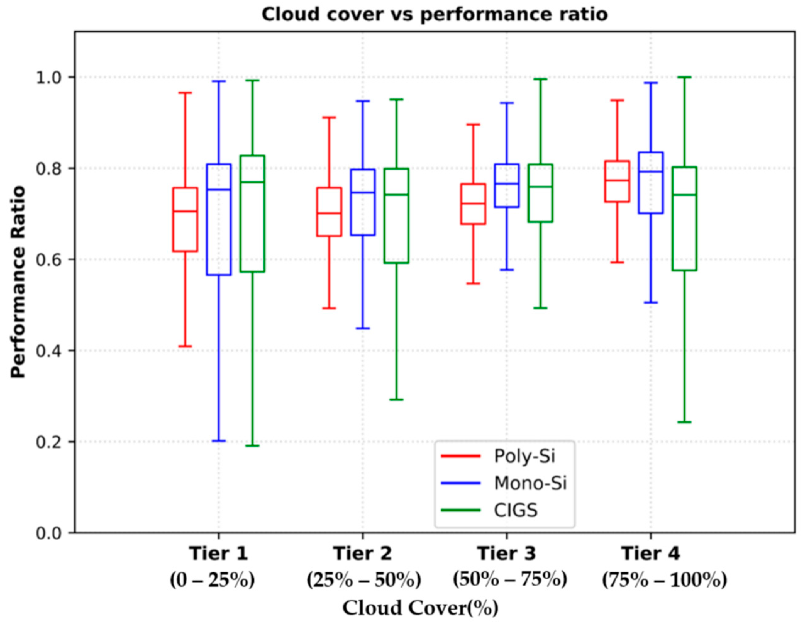
5.2. Comparison of Cloud Cover to Performance Ratio

To further investigate why CIGS has better PR than its counterparts in Louisiana, the impact of clouds on PR is examined. Cloud cover is plotted against PR to find the effect of clouds on the performance of PV modules. The value of cloud cover varies from 0% to 100%, with 0% indicating a clear sky and 100% indicating a sky completely covered by clouds. Cloud cover is put into four tiers: tier 1, tier 2, tier 3, and tier 4, in ranges of 0% to 25%, 25% to 50%, 50% to 75%, and 75% to 100%, respectively. Therefore, tier 1 represents the time when the sky is clear, and tier 4 represents the time when the sky is completely covered by clouds. Tier 2 and tier 3 represent intermediate clouds. For mono-Si and poly-Si arrays, the PR increases as the cloud cover increases, whereas for the CIGS array, the PR decreases with the increase in cloud cover, as shown in Figure 6.

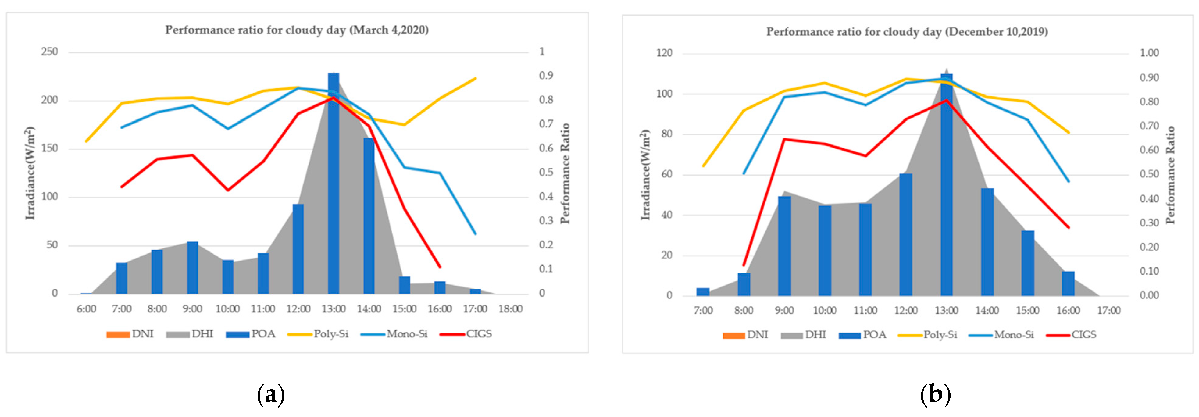
5.2.1. Performance Ratio for Clear Day and Cloudy Day

Figure 7 and Figure 8 shows the performance ratio for clear days and cloudy days, respectively. The two days (2 December 2019, 6 March 2020) represent typical clear days (tier 1) and similarly, the other two days (10 December 2019, 4 March 2020) represent typical cloudy days (tier 4). These days are chosen based on cloud cover percentage and irradiance. The figures also show the direct normal irradiance (DNI), diffuse horizontal irradiance (DHI), and plane of array irradiance (POA) for the chosen days.

CIGS has better PR than mono-Si and poly-Si on clear days (2 December and 6 March), as most of the POA irradiance constitutes DNI and a small portion from DHI. Poly-Si and mono-Si have better PR than CIGS on cloudy days (10 December and 4 March), as most of the POA irradiance constitutes DHI and a negligible portion from DNI. It can be inferred that CIGS, a type of thin-film module, performs worse in cloudy sky conditions (lower irradiance) unlike its counterpart CdTe, which is also a type of thin-film module that performs better in cloudy sky conditions.

5.2.2. Distribution of Clear and Cloudy Sky Hours for a Year

Having seen the performance of these technologies (mono-Si, poly-Si, and CIGS) on clear and cloudy days, it is important to determine the distribution of clear and cloudy sky hours for the analysed period (September 2019–August 2020), as shown in Figure 9a. For instance, 49% of the analysed period is in tier 1, and only 23% of the time is in tier 4. As the effect of clouds on PV during the night is insignificant, only the day hours are considered. As there are more hours with clear sky than cloud cover, CIGS has greater PR, as seen in Section 5.1.

5.2.3. Performance Ratio for December 2019 and January 2020

PR is unusually very high for CIGS compared to other technologies in December and January, especially in December where PR is 10% higher for CIGS than mono-Si and poly-Si. Figure 9b represents the distribution of clear and cloudy sky hours for December 2019 and January 2020, where it can be deduced that tier 1 and tier 4 comprise the same number of hours with clear and cloudy sky (42% each). It is expected to see the almost similar PR for all three technologies based on previous subsection, but PR is actually higher for CIGS than mono-Si and poly-Si, as shown in Figure 5. To investigate it, the energy yield and PR for these months are separated into four tiers, as shown in

Table 3. Average PR for each technology in each tier for December 2019 and January 2020.

	Poly-Si	Mono-Si	CIGS
Tier_1 (0–25%)	0.71	0.70	0.83
Tier_2 (25–50%)	0.73	0.76	0.82
Tier_3 (50–75%)	0.74	0.79	0.81
Tier_4 (75–100%)	0.76	0.79	0.79
Average	0.72	0.73	0.82

and

Table 4. Final yield (kWh/kW) for each technology in each tier for December 2019 and January 2020.

	Poly-Si	Mono-Si	CIGS	POA Insolation
Tier_1 (0–25%)	103.01	102.55	120.93	145.86 (64%)
Tier_2 (25–50%)	5.86	6.09	6.59	8.05 (3%)
Tier_3 (50–75%)	16.48	17.60	18.05	22.39 (10%)
Tier_4 (75–100%)	38.90	40.44	40.60	51.32 (23%)
Total	164.25	166.68	186.17	277.62 (100%)

.

It can be inferred from Table 3 that there is a significant rise in PR for mono-Si and poly-Si and a small decrease in PR for CIGS as cloud cover increases from 0% to 100%. From Table 4, it can be inferred that tier 1 and tier 4 constitute 64% and 23% of total POA insolation, respectively. The final yield for CIGS is much higher than mono-Si and poly-Si in tier 1. A very small difference in final yield for the three technologies is observed in tier 4. Although tier 1 and tier 4 comprise the same number of hours with clear and cloudy sky, the insolation weightage is higher in tier 1 than tier 4. Hence CIGS performed significantly better than mono-Si and poly-Si in December 2019 and January 2020.

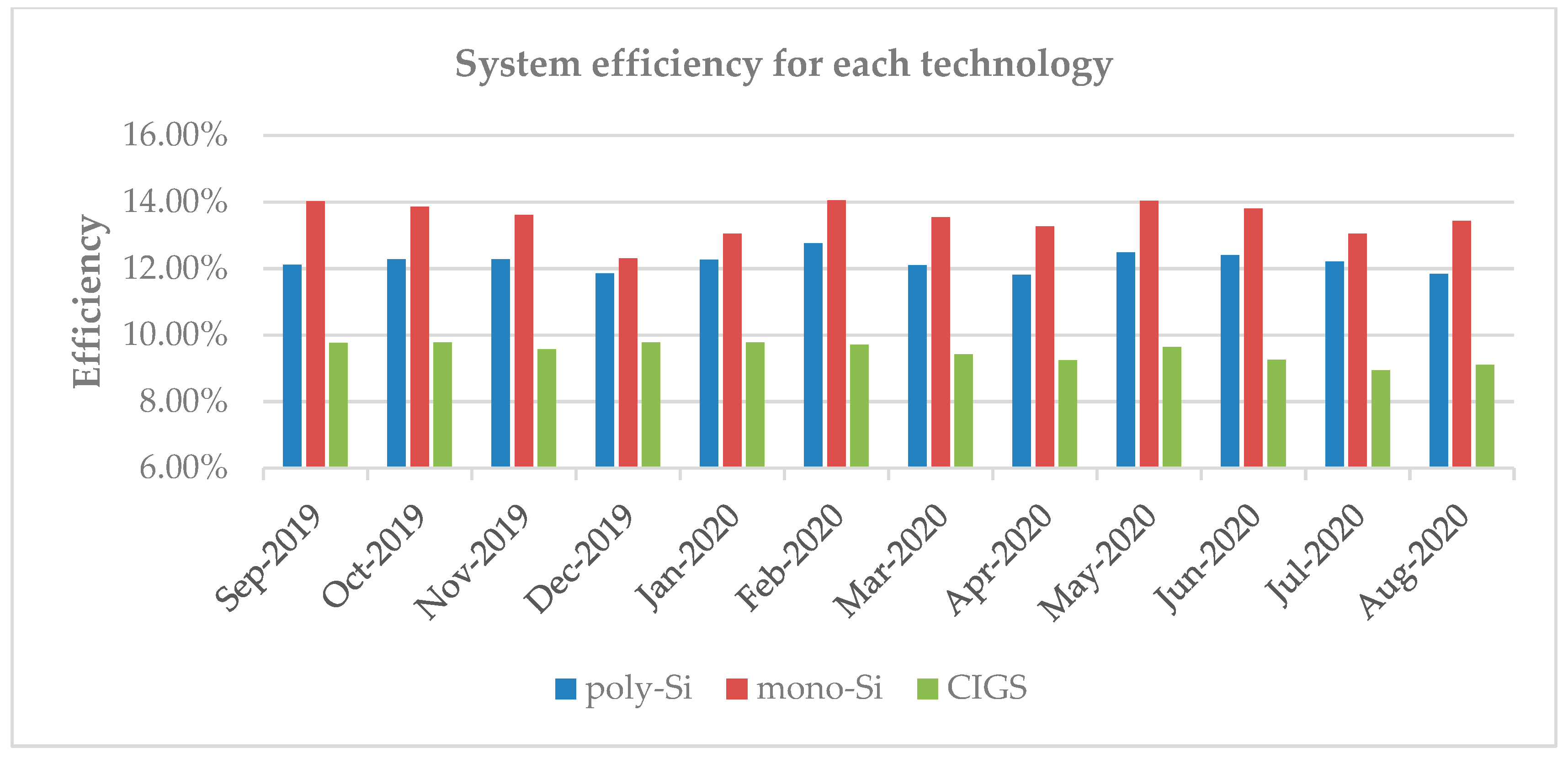
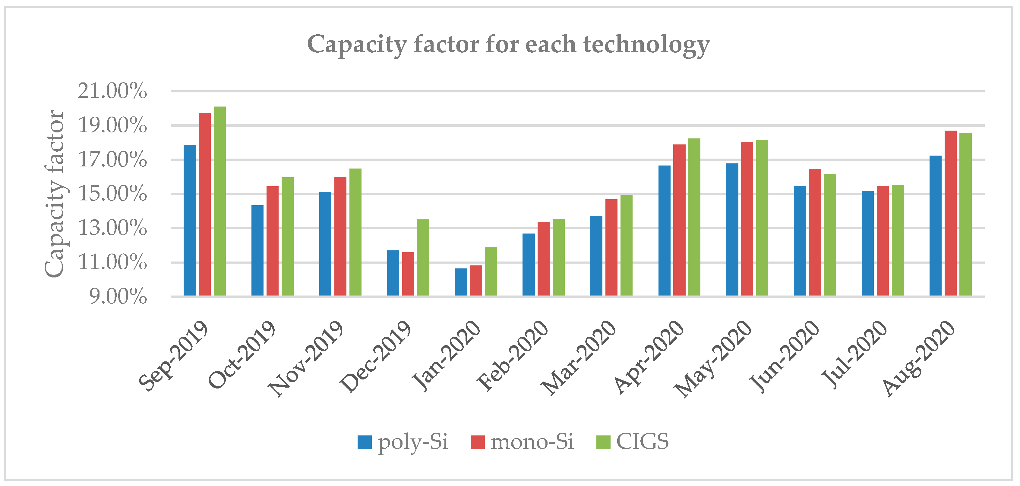
5.3. System Efficiency and Capacity Factor

The system efficiency for mono-Si technology varies from 12.30% to 14.04% over different months, as shown in Figure 10. For poly-Si technology, system efficiency varies from 11.80% to 12.76%, whereas the CIGS has a small variation for different months from 8.94% to 9.78%. Mono-Si technology has an average yearly efficiency of 13.50% and has better efficiency than poly-Si and CIGS as expected, which have an average yearly efficiency of 12.20%, and 9.50%, respectively.

The average value of capacity factor in Figure 11 for poly-Si, mono-Si, and the CIGS are 14.78%, 15.68%, and 16.08%, respectively. The CIGS has better capacity factor compared with the other two technologies. The variation in the capacity factor is due to the system losses because of local climatic conditions. The capacity factor was lower during the months of December and January because this location had lower insolation during these months.

5.4. Economic Analysis

Figure 12 shows the distribution of installation costs between modules, inverters, and the balance of the system. The power plant was built at a cost of $1.40 per Watt. Although the land is owned by the university, the land cost was assumed to be $3569 per acre for the analysis [39]. For poly-Si technology, modules cost an average of $0.42 per Watt and inverters cost $0.08 per Watt. For mono-Si technology, modules cost $0.53 per Watt and inverters cost $0.18 per Watt. For CIGS, modules cost $0.59 per Watt and inverters cost $0.18 per Watt. Inverters for mono-Si and CIGS were more expensive because they have power optimizers. Maintenance costs were assumed to be $17,000/MW per year.

Discounted levelized cost of energy (LCOE) is calculated using Equation (8) at an interest rate of 3%, which is the Department of Energy (DOE) discount rate for projects related to energy conservation and renewable energy for 2018 [40]. The lifecycle of the powerplant is considered to be 25 years, which is the standard lifetime of any solar PV plant [37]. Energy generated was extrapolated for the life of the project from the first two years of energy production. The degradation rate for crystalline silicon modules and CIGS was assumed to be 0.5% [41,42].

Overall, the powerplant has an expected LCOE of 80 $/MWh, which is high compared to the published Lazard LCOE of $40 to $46 for utility scale because of the smaller system size, resulting in a relatively high capital cost for this project [43]. Poly-Si has the lowest LCOE of 79 $/MWh compared to mono-Si and CIGS, which have LCOEs of 86 $/MWh and 86 $/MWh, respectively, as shown in Figure 13. Although CIGS has a slightly higher LCOE, it could have been potentially lower with a larger installation size.

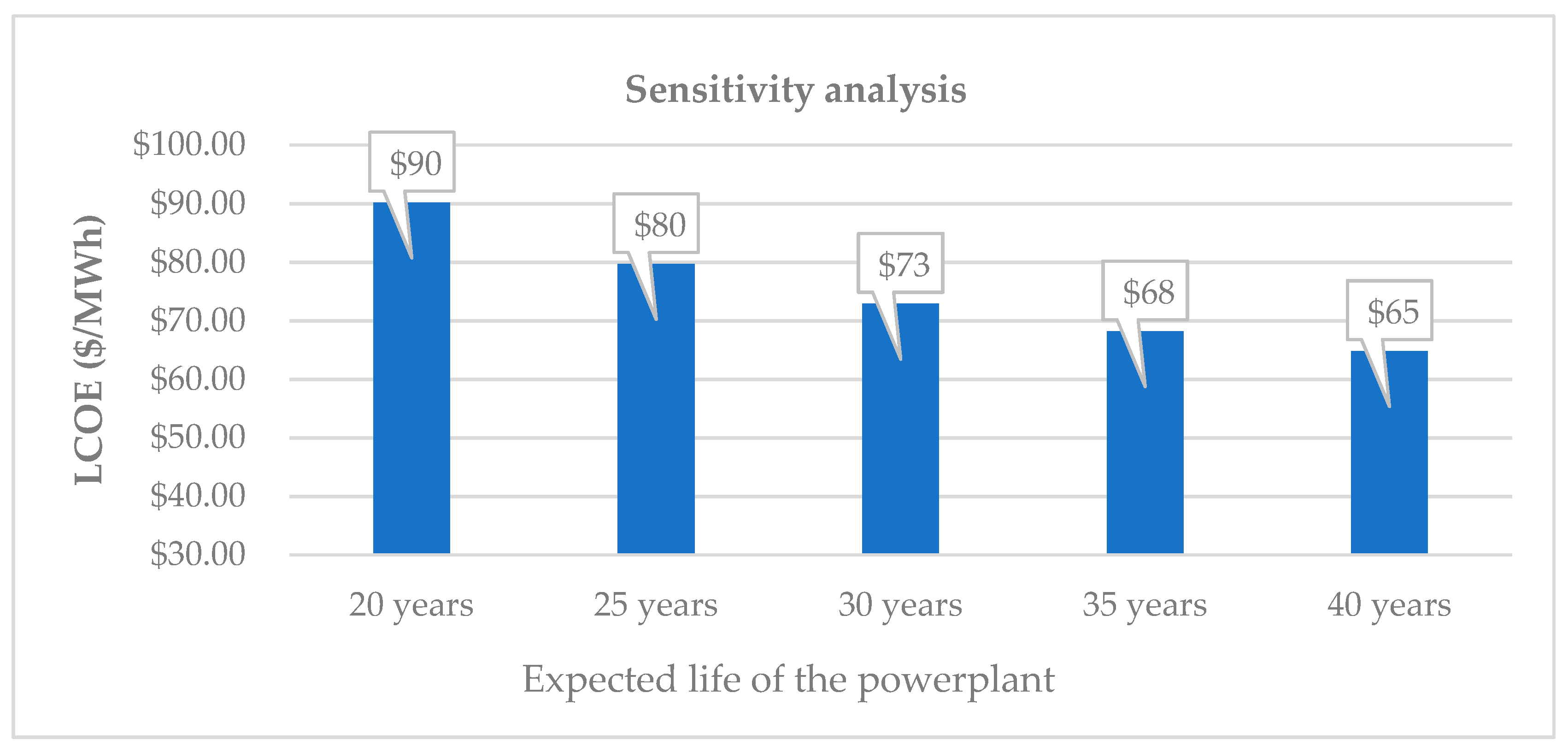
5.5. Sensitivity Analysis

LCOE strongly depends on the life of the project. Although the life of the project is assumed to be 25 years, it can vary greatly based on solar panel’s performance. Most solar panel manufacturers give a warranty of 80% retained power output after 20 years of operation. Therefore, the sensitivity analysis is done for LCOE by varying the expected life of the project from 20 years to 40 years, as shown in Figure 14. LCOE is 90$/MWh if the project is decommissioned in 20 years, which is very high. There is a steep decrease in LCOE when the life of the project increases from 20 years to 30 years and then gradually decreases, reaching a low of 65$/MWh if the project lasts 40 years.

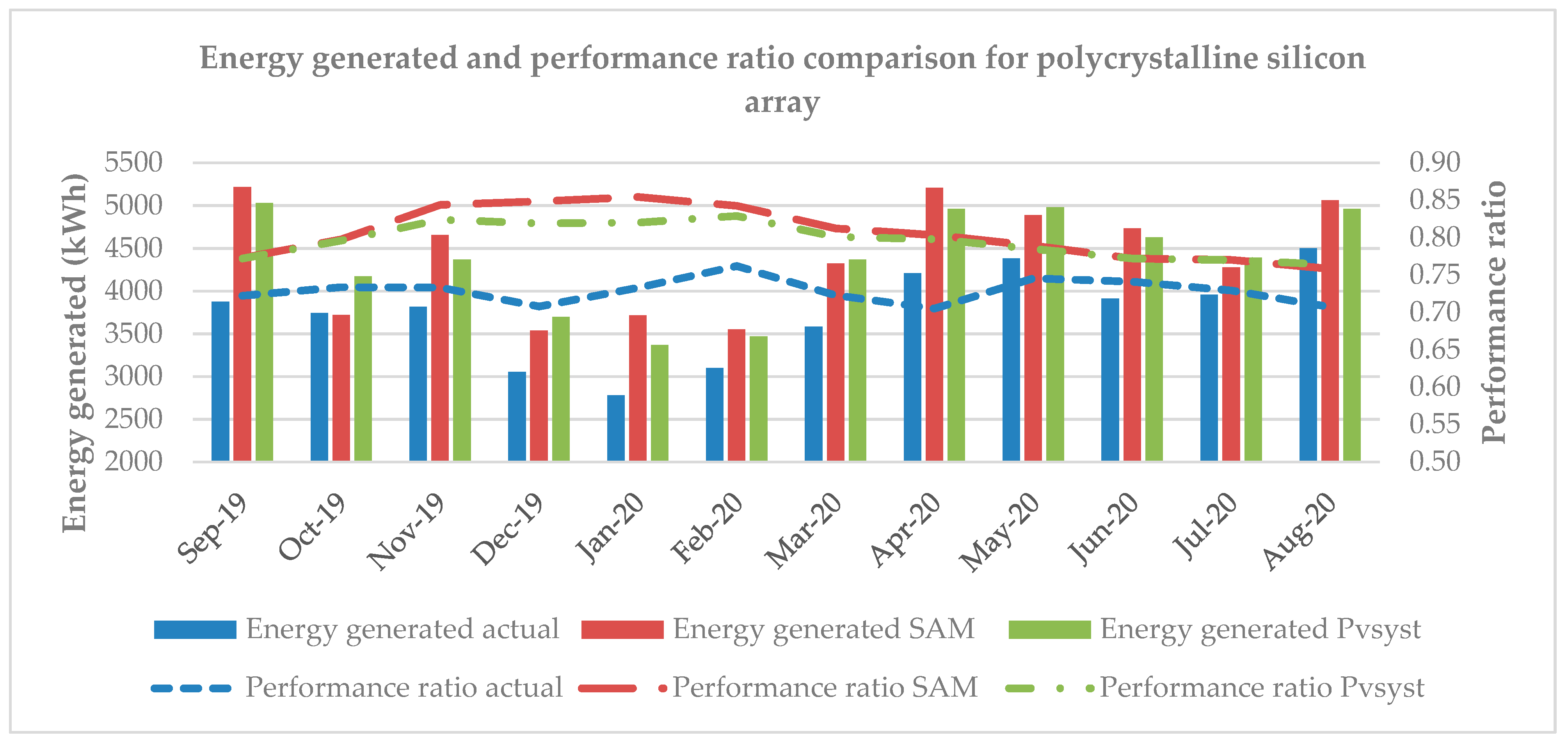
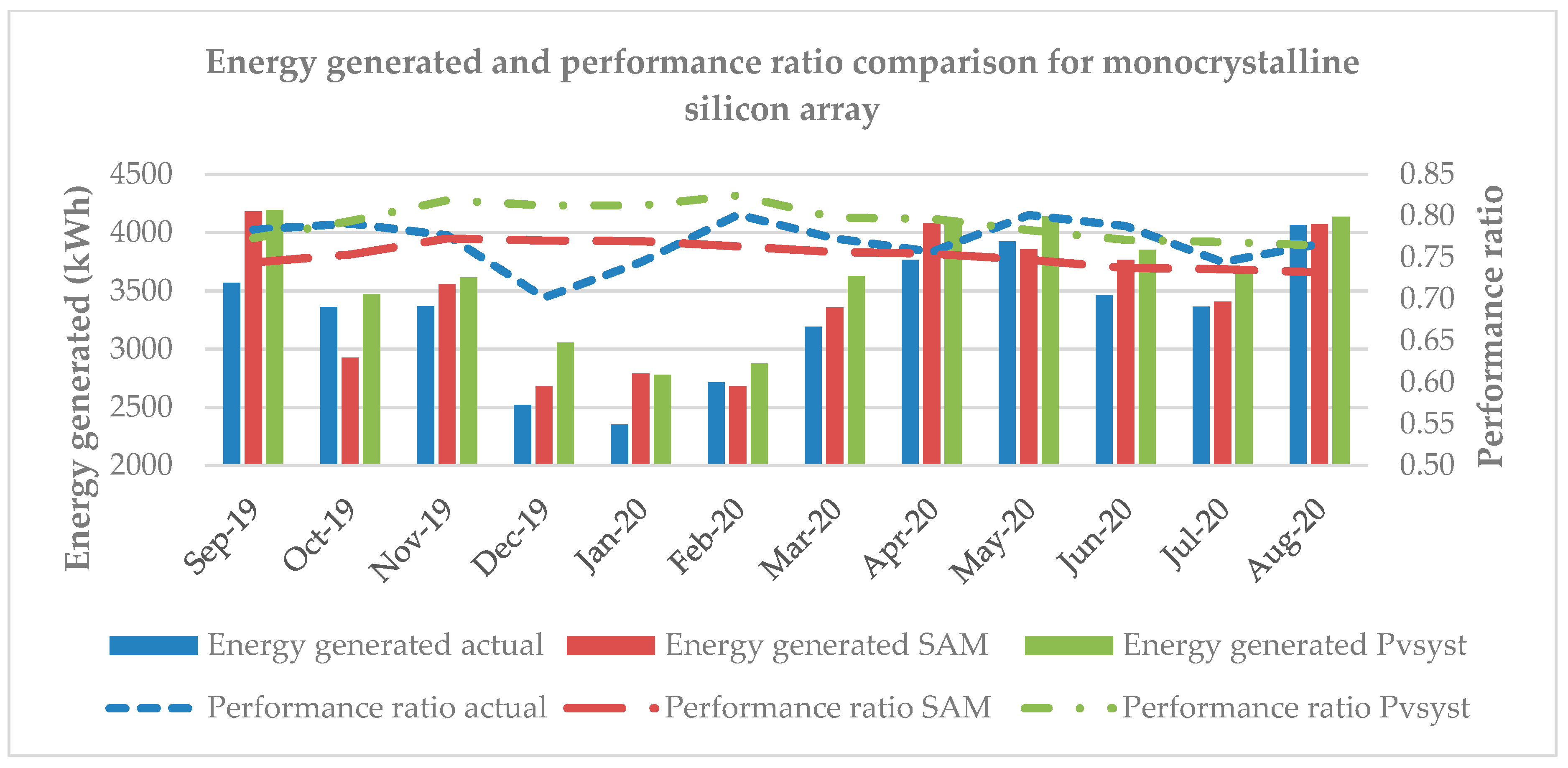
5.6. Comparison of Actual Data to Simulation Results

In this section, performance data from the field are compared with the modelled data from SAM and PVsyst. Figure 15, Figure 16 and Figure 17 show the comparison of actual to simulated energy generated and the PR for three PV technologies.

For the poly-Si array, the simulation values using SAM and PVsyst are greater than the actual energy yield. Similarly, the PR is also lower compared with the simulated values. For mono-Si array, the actual energy yield is less than the simulated values. Actual PR is in accordance with SAM results, except during the month of December. The PR predicted using PVsyst is greater than simulation values using SAM.

The CIGS has an actual energy yield and PR closer to the simulation values using PVsyst. Simulation values using SAM show a larger variation from actual values for most of the months. The variation may be because PVsyst is able to simulate the thin film system with power optimizers better than SAM.

To find the accuracy of simulation models, NMAE and NMBE were calculated for AC energy, and results are shown in

Table 5. Error values of simulation using SAM and PVsyst.

	Error Values in AC Energy Calculation for Simulation Using SAM			Error Values in AC Energy Calculation for Simulation Using PVsyst
Technology	NMBE (%)	NMAE (%)	R2	NMBE (%)	NMAE (%)	R2
Poly-Si	14.76	14.84	0.70	13.85	13.85	0.87
Mono-Si	3.46	5.65	0.78	7.91	7.91	0.90
CIGS	−7.23	8.41	0.39	2.91	3.40	0.90

. NMBE is positive for simulation using PVsyst, and poly-Si has the largest error in calculating the energy using PVsyst. PVsyst consistently overpredicted the energy for all three technologies, whereas SAM overpredicted for poly-Si and mono-Si and underpredicted for CIGS. Overall, the mean bias error for SAM is greater than PVsyst. These differences can be attributed to level of detail required by the inputs into each software. PVsyst is a more technically in-depth software requiring more inputs than SAM. Although the biased error and absolute error are high due to differences in insolation from satellite-based measurements, a regression coefficient of more than 0.85 indicates that PVsyst performed well in predicting the energy generated. Another source of error could be the discrepancies in the measured POA irradiance and the satellite-based irradiance.

In summary, simulated results using SAM are in accordance with actual values for mono-Si, and simulation using PVsyst are in accordance with the CIGS.

5.7. Comparison with Other Studies

Table 6. Comparison of performance of different PV systems.

Location	Climate Classification	PV Type a	Installed Capacity (kW)	Final Yield (kWh/kW)	System Efficiency (%)	Performance Ratio (%)	Capacity Factor (%)	Reference
Mauritania	Arid (B)	Micromorph-Si (Array 1)	954.72 kW	4.29	NA b	67.90%	17.75%	[44]
Kuwait	Arid subtropical (B)	Poly-Si	5.6 MW	5.18	13.02%	80.20%	20.66%	[17]
Kuwait	Arid subtropical (B)	Thin film	5.5 MW	5.16	10.42%	80%	20.61%	[17]
India	Desert, semi arid (B)	Mono-Si	3 MW	3.73	NA	70%	NA	[10]
Algeria	Hot desert (bwh)	Poly-Si	6 MW	5.15	11.39%	73.70%	21.44%	[32]
Greece	Temperate	Poly-Si	171.36 kW	3.66	NA	67.40%	15.30%	[45]
Italy (42 months)	Temperate	Mono-Si	960 kW	3.8	14.90%	84.40%	15.66%	[30]
Malawi (4 years)	Temperate	HIT	830 kW	4.25	14.60%	79.50%	17.70%	[29]
India	Temperate (humid subtropical)	Poly-Si	10 MW	NA	NA	86.10%	17.70%	[14]
India	Temperate (humid, subtropical)	Poly-Si	190 kW	2.23	8.30%	74%	9.27%	[12]
Aratiba, RS, Brazil	Temperate (humid, subtropical)	Poly-Si, mono-Si, CIGS,	54 kW	NA	NA	79%, 79%, 76%	NA	[26]
Capivari de Baixo, SC, Brazil	Temperate (humid, subtropical)	Poly-Si, mono-Si, CIGS	54 kW	NA	NA	75%, 79%, 76%	NA	[26]
Louisiana, USA c	Temperate (humid, subtropical)	CIGS d	20.28 kW	3.81	9.50%	79%	16.08%	Current research
Louisiana, USA c	Temperate (humid, subtropical)	mono-Si	147.56 kW	3.72	13.50%	77%	15.68%	Current research
Louisiana, USA c	Temperate (humid, subtropical)	Poly-Si	1.15 MW	3.5	12.20%	73%	14.78%	Current research
Ghana (3 years)	Tropical	Poly-Si	2.5 MW	NA	NA	70.60%	16.20%	[37]
India	tropical	A-Si	5 MW	4.81	5.08%	89.20%	NA	[15]
India (four years)	Tropical semiarid	Mono-Si	1 MW	4.64	11.02%	74.73%	19.33%	[13]

^a PV—photovoltaic. ^b NA—not available. ^c USA—United States of America. ^d CIGS—cadmium indium gallium selenide.

shows the comparison of performance parameters for similar PV systems all over the world. Final yield per day for the current study is slightly lower compared with other studies, which is caused by lower insolation at the current location. For temperate climate, poly-Si and mono-Si have a lower PR of 73% and 76%, respectively, compared to the other reported values in India and Brazil [12,14,26]. CIGS has comparatively better performance ratio of 79% compared to a study in Brazil [26]. In general, the current powerplant has performed reasonably well relative to other research in all climates, with a performance ratio of more than 70% for all technologies. The capacity factor of 14–16% is consistent with previous temperate climate findings, indicating that the powerplant is operating commensurately.

6. Conclusions

In this study, the performance of the 1.1 MW powerplant in Lafayette, Louisiana, was evaluated, and three different module technologies were compared based on the monthly final yield, PR, capacity factor, and system efficiency.

• The plant has produced 3.1 GWh of energy as of August 2020, which is equivalent to saving 1.4 million gallons of water; it has also generated a CO₂ offset equivalent of planting 54,764 trees.
• The CIGS has a PR of 0.79 in this period, which is better than the other two technologies.
• It was also found that the CIGS has better PR than the crystalline silicon technology on clear days.
• In terms of system efficiency, the mono-Si array has better efficiency (13.50%) than the poly-Si array (12.20%), and the CIGS array (9.50%).
• Poly-Si has the lowest LCOE of 79$/MWh compared to other technologies.
• Simulation results for the mono-Si and CIGS are much closer to actual values, whereas actual values are lower than the simulation for poly-Si.

The CIGS has the highest yield per kW STC, mainly due to having the lowest dependence on temperature for efficiency. In Louisiana, the average temperature during the day is high, ranging from 15 °C to 29 °C. With the highest PR, capacity factor, and potentially lower LCOE for bigger installations, CIGS is better in these conditions.

These findings suggest that any future solar plant installed in Louisiana can operate with a good amount of PR and system efficiency. The monitored data and operating experience of the PV system can be applied for future large-scale projects. It is recommended that future studies explore long-term degradation for these three technologies.

References

1. Solar Market Insight Report 2018 Year in Review|SEIA. Available online: https://www.seia.org/research-resources/solar-market-insight-report-2018-year-review (accessed on 23 March 2021).
2. Solar Market Insight Report 2019 Year in Review|SEIA. Available online: https://www.seia.org/research-resources/solar-market-insight-report-2019-year-review (accessed on 23 March 2021).
3. Louisiana Solar|SEIA. Available online: https://www.seia.org/state-solar-policy/louisiana-solar (accessed on 23 March 2021).
4. Memiche, M.; Bouzian, C.; Benzahia, A.; Moussi, A. Effects of dust, soiling, aging, and weather conditions on photovoltaic system performances in a Saharan environment—Case study in Algeria. Glob. Energy Interconnect. 2020, 3, 60–67. [Google Scholar] [CrossRef]
5. Kurnik, J.; Jankovec, M.; Brecl, K.; Topic, M. Outdoor testing of PV module temperature and performance under different mounting and operational conditions. Sol. Energy Mater. Sol. Cells 2011, 95, 373–376. [Google Scholar] [CrossRef]
6. Marion, B.; Adelstein, J.; Boyle, K.; Hayden, H.; Hammond, B.; Fletcher, T.; Canada, B.; Narang, D.; Kimber, A.; Mitchell, L.; et al. Performance parameters for grid-connected PV systems. In Proceedings of the IEEE Conference Record of the Thirty-First IEEE Photovoltaic Specialists Conference, Lake Buena Vista, FL, USA, 3–7 January 2005; pp. 1601–1606. [Google Scholar] [CrossRef] [Green Version]
7. Magare, D.; Sastry, O.S.; Gupta, R.; Betts, T.R.; Gottschalg, R.; Kumar, A.; Bora, B.; Singh, Y.K. Effect of seasonal spectral variations on performance of three different photovoltaic technologies in India. Int. J. Energy Environ. Eng. 2016, 7, 93–103. [Google Scholar] [CrossRef] [Green Version]
8. Jamil, I.; Zhao, J.; Zhang, L.; Jamil, R.; Rafique, S.F. Evaluation of Energy Production and Energy Yield Assessment Based on Feasibility, Design, and Execution of 3 × 50 MW Grid-Connected Solar PV Pilot Project in Nooriabad. Int. J. Photoenerg. 2017, 2017, 6429581. [Google Scholar] [CrossRef] [Green Version]
9. Durisch, W.; Bitnar, B.; Mayor, J.C.; Kiess, H.; Lam, K.H.; Close, J. Efficiency model for photovoltaic modules and demonstration of its application to energy yield estimation. Sol. Energy Mater. Sol. Cells 2007, 91, 79–84. [Google Scholar] [CrossRef]
10. Padmavathi, K.; Daniel, S.A. Performance analysis of a 3MWp grid connected solar photovoltaic power plant in India. Energy Sustain. Dev. 2013, 17, 615–625. [Google Scholar] [CrossRef]
11. Verma, S.; Yadav, D.K.; Sengar, N. Performance Evaluation of Solar Photovoltaic Power Plants of Semi-Arid Region and Suggestions for Efficiency Improvement. Int. J. Renew. Energy Res. 2021, 11, 762–775. [Google Scholar]
12. Sharma, V.; Chandel, S. Performance analysis of a 190 kWp grid interactive solar photovoltaic power plant in India. Energy 2013, 55, 476–485. [Google Scholar] [CrossRef]
13. Malvoni, M.; Kumar, N.M.; Chopra, S.S.; Hatziargyriou, N. Performance and degradation assessment of large-scale grid-connected solar photovoltaic power plant in tropical semi-arid environment of India. Sol. Energy 2020, 203, 101–113. [Google Scholar] [CrossRef]
14. Kumar, B.S.; Sudhakar, K. Performance evaluation of 10 MW grid connected solar photovoltaic power plant in India. Energy Rep. 2015, 1, 184–192. [Google Scholar] [CrossRef] [Green Version]
15. Sundaram, S.; Babu, J.S.C. Performance evaluation and validation of 5MWp grid connected solar photovoltaic plant in South India. Energy Convers. Manag. 2015, 100, 429–439. [Google Scholar] [CrossRef]
16. Bansal, N.; Pany, P.; Singh, G. Visual degradation and performance evaluation of utility scale solar photovoltaic power plant in hot and dry climate in western India. Case Stud. Therm. Eng. 2021, 26, 101010. [Google Scholar] [CrossRef]
17. Al-Rasheedi, M.; Gueymard, C.A.; Al-Khayat, M.; Ismail, A.; Lee, J.A.; Al-Duaj, H. Performance evaluation of a utility-scale dual-technology photovoltaic power plant at the Shagaya Renewable Energy Park in Kuwait. Renew. Sustain. Energy Rev. 2020, 133, 110139. [Google Scholar] [CrossRef]
18. Martín-Martínez, S.; Cañas-Carretón, M.; Honrubia-Escribano, A.; Gómez-Lázaro, E. Performance evaluation of large solar photovoltaic power plants in Spain. Energy Convers. Manag. 2019, 183, 515–528. [Google Scholar] [CrossRef]
19. Schweiger, M.; Herrmann, W.; Gerber, A.; Rau, U. Understanding the energy yield of photovoltaic modules in different climates by linear performance loss analysis of the module performance ratio. IET Renew. Power Gener. 2017, 11, 558–565. [Google Scholar] [CrossRef]
20. Adouane, M.; Al-Qattan, A.; Alabdulrazzaq, B.; Fakhraldeen, A. Comparative performance evaluation of different photovoltaic modules technologies under Kuwait harsh climatic conditions. Energy Rep. 2020, 6, 2689–2696. [Google Scholar] [CrossRef]
21. Muehleisen, W.; Loeschnig, J.; Feichtner, M.; Burgers, A.; Bende, E.; Zamini, S.; Yerasimou, Y.; Kosel, J.; Hirschl, C.; Georghiou, G. Energy yield measurement of an elevated PV system on a white flat roof and a performance comparison of monofacial and bifacial modules. Renew. Energy 2021, 170, 613–619. [Google Scholar] [CrossRef]
22. Saber, E.; Lee, S.E.; Manthapuri, S.; Yi, W.; Deb, C. PV (photovoltaics) performance evaluation and simulation-based energy yield prediction for tropical buildings. Energy 2014, 71, 588–595. [Google Scholar] [CrossRef]
23. Wittkopf, S.K.; Valliappan, S.; Liu, L.; Ang, K.S.; Cheng, S.C.J. Analytical performance monitoring of a 142.5kWp grid-connected rooftop BIPV system in Singapore. Renew. Energy 2012, 47, 9–20. [Google Scholar] [CrossRef]
24. Romero-Fiances, I.; Muñoz-Cerón, E.; Espinoza-Paredes, R.; Nofuentes, G.; De la Casa, J. Analysis of the Performance of Various PV Module Technologies in Peru. Energies 2019, 12, 186. [Google Scholar] [CrossRef] [Green Version]
25. Chimtavee, A.; Ketjoy, N. PV Generator Performance Evaluation and Load Analysis of the PV Microgrid System in Thailand. Procedia Eng. 2012, 32, 384–391. [Google Scholar] [CrossRef] [Green Version]
26. Nascimento, L.R.D.; Braga, M.; Campos, R.A.; Naspolini, H.F.; Rüther, R. Performance assessment of solar photovoltaic technologies under different climatic conditions in Brazil. Renew. Energy 2020, 146, 1070–1082. [Google Scholar] [CrossRef]
27. De Lima, L.C.; Ferreira, L.D.A.; de Lima Morais, F.H.B. Performance analysis of a grid connected photovoltaic system in northeastern Brazil. Energy Sustain. Dev. 2017, 37, 79–85. [Google Scholar] [CrossRef]
28. Ameur, A.; Sekkat, A.; Loudiyi, K.; Aggour, M. Performance evaluation of different photovoltaic technologies in the region of Ifrane, Morocco. Energy Sustain. Dev. 2019, 52, 96–103. [Google Scholar] [CrossRef]
29. Banda, M.H.; Nyeinga, K.; Okello, D. Performance evaluation of 830 kWp grid-connected photovoltaic power plant at Kamuzu International Airport-Malawi. Energy Sustain. Dev. 2019, 51, 50–55. [Google Scholar] [CrossRef]
30. Malvoni, M.; Leggieri, A.; Maggiotto, G.; Congedo, P.M.; de Giorgi, M.G. Long term performance, losses and efficiency analysis of a 960 kW P photovoltaic system in the Mediterranean climate. Energy Convers. Manag. 2017, 145, 169–181. [Google Scholar] [CrossRef]
31. Abdullah, G.; Nishimura, H. Techno-Economic Performance Analysis of a 40.1 kWp Grid-Connected Photovoltaic (GCPV) System after Eight Years of Energy Generation: A Case Study for Tochigi, Japan. Sustainability 2021, 13, 7680. [Google Scholar] [CrossRef]
32. Dahbi, H.; Aoun, N.; Sellam, M. Performance analysis and investigation of a 6 MW grid-connected ground-based PV plant installed in hot desert climate conditions. Int. J. Energy Environ. Eng. 2021, 12, 577–587. [Google Scholar] [CrossRef]
33. Tozzi, P.; Jo, J.H. A comparative analysis of renewable energy simulation tools: Performance simulation model vs. system optimization. Renew. Sustain. Energy Rev. 2017, 80, 390–398. [Google Scholar] [CrossRef]
34. De Souza Silva, J.L.; Costa, T.S.; de Melo, K.B.; Sako, E.Y.; Moreira, H.S.; Villalva, M.G. A Comparative Performance of PV Power Simulation Software with an Installed PV Plant. In Proceedings of the 2020 IEEE International Conference on Industrial Technology (ICIT), Buenos Aires, Argentina, 26–28 February 2020; pp. 531–535. [Google Scholar] [CrossRef]
35. Ayompe, L.M.; Duffy, A.; McCormack, S.J.; Conlon, M. Measured performance of a 1.72kW rooftop grid connected photovoltaic system in Ireland. Energy Convers. Manag. 2011, 52, 816–825. [Google Scholar] [CrossRef] [Green Version]
36. Mondol, J.D.; Yohanis, Y.G.; Norton, B. The effect of low insolation conditions and inverter oversizing on the long-term performance of a grid-connected photovoltaic system. Prog. Photovolt. Res. Appl. 2007, 15, 353–368. [Google Scholar] [CrossRef]
37. Mensah, L.D.; Yamoah, J.O.; Adaramola, M.S. Performance evaluation of a utility-scale grid-tied solar photovoltaic (PV) installation in Ghana. Energy Sustain. Dev. 2019, 48, 82–87. [Google Scholar] [CrossRef]
38. Dahmoun, M.E.-H.; Bekkouche, B.; Sudhakar, K.; Guezgouz, M.; Chenafi, A.; Chaouch, A. Performance evaluation and analysis of grid-tied large scale PV plant in Algeria. Energy Sustain. Dev. 2021, 61, 181–195. [Google Scholar] [CrossRef]
39. Texas Real Estate Research Center. Rural Land Prices for Louisiana. Available online: https://www.recenter.tamu.edu/data/rural-land/#!/state/Louisiana (accessed on 2 May 2022).
40. Lavappa, P.D.; Kneifel, J.D. Energy Price Indices and Discount Factors for Life-Cycle Cost Analysis—2018 Annual Supplement to NIST Handbook 135; National Institute of Standards and Technology: Gaithersburg, MD, USA, 2018; NIST IR 85-3273-33. [Google Scholar] [CrossRef]
41. Jordan, D.C.; Kurtz, S.R. Photovoltaic Degradation Rates-an Analytical Review: Photovoltaic degradation rates. Prog. Photovolt. Res. Appl. 2013, 21, 12–29. [Google Scholar] [CrossRef] [Green Version]
42. King, B.H.; Stein, J.S.; Riley, D.; Jones, C.B.; Robinson, C.D. Degradation Assessment of Fielded CIGS Photovoltaic Arrays. In Proceedings of the 2017 IEEE 44th Photovoltaic Specialist Conference (PVSC), Washington, DC, USA, 25–30 June 2017; pp. 3155–3160. [Google Scholar] [CrossRef]
43. Lazard. Levelized Cost of Energy and Levelized Cost of Storage. 2018. Available online: https://www.lazard.com/perspective/levelized-cost-of-energy-and-levelized-cost-of-storage-2018/ (accessed on 23 March 2021).
44. Sidi, C.E.B.E.; Ndiaye, M.L.; El Bah, M.; Mbodji, A.; Ndiaye, A.; Ndiaye, P.A. Performance analysis of the first large-scale (15 MWp) grid-connected photovoltaic plant in Mauritania. Energy Convers. Manag. 2016, 119, 411–421. [Google Scholar] [CrossRef]
45. Kymakis, E.; Kalykakis, S.; Papazoglou, T.M. Performance analysis of a grid connected photovoltaic park on the island of Crete. Energy Convers. Manag. 2009, 50, 433–438. [Google Scholar] [CrossRef]
Figure 1. Layout of 1.1 MW solar photovoltaic power plant at the University of Louisiana, Lafayette.
Energies 15 03420 g001
Figure 2. Simplified block diagram of photovoltaic power plant in University of Louisiana, Lafayette.
Energies 15 03420 g002
Figure 3. Line diagram of high voltage panels (HP) and distribution panels (DP).
Energies 15 03420 g003
Figure 4. Ambient temperature and insolation from September 2019 to August 2020.
Energies 15 03420 g004
Figure 5. Performance ratio comparison for three PV technologies.
Energies 15 03420 g005
Figure 6. Cloud cover vs. performance ratio.
Energies 15 03420 g006
Figure 7. Performance ratio and irradiance on clear days: (a) 2 December 2019 (b) 6 March 2020.
Energies 15 03420 g007
Figure 8. Performance ratio and irradiance on cloudy days: (a) 10 December 2019 (b) 4 March 2020.
Energies 15 03420 g008
Figure 9. (a) Percentage of time spent in each cloud cover band for a year; (b) percentage of time spent in each cloud cover band for December 2019 and January 2020.
Energies 15 03420 g009
Figure 10. System efficiency for each technology.
Energies 15 03420 g010
Figure 11. Capacity factor for each technology.
Energies 15 03420 g011
Figure 12. System cost for the power plant.
Energies 15 03420 g012
Figure 13. Discounted LCOE for each technology.
Energies 15 03420 g013
Figure 14. Sensitivity analysis of LCOE.
Energies 15 03420 g014
Figure 15. Comparison of actual energy generated and performance ratio to simulated values for polycrystalline silicon array.
Energies 15 03420 g015
Figure 16. Comparison of actual energy generated and performance ratio to simulated values for monocrystalline silicon array.
Energies 15 03420 g016
Figure 17. Comparison of actual energy generated and performance ratio to simulated values for CIGS array.
Energies 15 03420 g017