Effect of the Design Parameters of the Combustion Chamber on the Efficiency of a Thermal Oxidizer

Abstract

Carbon monoxide is often produced during the incomplete combustion of volatile organic carbon compounds in industry. In the combustion chamber for oxidizing carbon monoxide emissions, a penta-coaxial port device can be used to improve the process of mixing the fuel and oxidizer. In this study, the conjugate heat transfer analysis was conducted by solving both Reynolds-averaged Navier–Stokes equations with the eddy dissipation model and solid heat conduction equation in the wall using Fluent 2019R2 to simulate the reaction flow of a volatile organic carbon compound burner and heat transfer of the stack insulation layer. The mass fractions of the O₂, CO₂, and CO gases; the temperature; and the velocity distribution in a combustion chamber were computed to investigate how various design parameters of the combustor, including air inlet size and stack height, and air inflow conditions affected the combustion performance. Results show that the size of the air inlet had only a minor effect on combustion efficiency and that the airstream forced by a fan significantly enhanced the combustion performance. In particular, increasing the height of the stack from 2 m to 4 m greatly increased combustion efficiency from 63% to 94%, with a 50% increase in the incoming air flow rate by natural convection, which demonstrates the importance of stack height in combustor design.

1. Introduction

Volatile organic compounds (VOCs) are organic chemicals that usually contain both hydrogen and carbon elements. They are harmful contaminants that are emitted into the environment as a result of various commercial and industrial processes [1]. Carbon monoxide is a colorless, odorless, and tasteless gas that is created by the incomplete combustion of fuels such as gasoline, natural gas, oil, coal, and wood. Although carbon monoxide does not have a significant environmental effect, in general, it can react with other air pollutants and have a negative effect on the ozone layer. A VOC burner can oxidize the organic components into water and carbon dioxide. Most VOC burners operate by blowing air and fuels into the combustor (forced combustor), but some types of combustors, such as stone gas, torch, and Bunsen burners, can work well without blowing air or a fan. These devices operate using density differences caused by temperature change, and the airflow automatically enters the chamber by natural convection. The aim in this study was to use computational fluid dynamics (CFD) to investigate the performance of non-premixed combustion in thermal oxidizers with various burner design configurations.

In a previous work, Das et al. [2] numerically studied heat transfer and air flow by natural convection in a solar updraft tower. They showed that the chimney height significantly affects the air flow rate, with a 31% increase when the chimney height was increased from 3 m to 8 m.

Pundle et al. [3] conducted numerical simulations in STAR-CCM software to predict the performance of natural draft rocket cookstoves. They combined the realizable k−ε turbulence model with the laminar finite rate model for combustion. They found that the air flow rate was affected by geometrical design features such as the height of the pot cone-deck and the baffle position.

Lee et al. [4] investigated the characteristics and structure of palm-methyl-ester diffusion flames and showed that the stability of the lifted flame depends on the edge propagation speed, mixture strength, and fuel Lewis number in the jet-momentum-dominated regime and that the effect of buoyancy on the stability of the lifted flame is negligible in developed regions.

The fuel-to-air ratio is a key factor affecting gas emissions. Qian et al. [5] suggested that an excess air (EA) ratio in the range of 0.04 to 0.79 reduces CO and SO₂ emissions and increases nitrogen oxide (NOx) production. On the contrary, an EA ratio above 0.79 lowers NOx emissions and increases CO and SO₂. Al-Arkawazi [6] studied the effect of the air–fuel ratio and lambda (λ) on the exhaust emissions from internal combustion engines and provided a curve of direct relationship between them.

The numerical approach to thermal–fluid reaction flow has been applied in a wide range of engineering fields and it works well for predicting the phenomena of combustion [3,7,8,9,10,11,12,13]. However, studies including detailed flow characteristics of natural combustion in a VOC burner with a stack are rare. In this work, the conjugate heat transfer analysis was conducted to investigate how various design parameters of the combustor and air flow conditions affect the combustion efficiency and the performance of the wall insulation layer.

1.1. Classification of Burners

The flow characteristics of an inverse diffusion flame (IDF) during the transition from laminar to turbulent flow were studied by Zhen et al. [14]. They concluded that the flames were affected by the burner geometry, chemical reaction parameters, and fuel/oxidizer fluid dynamics. Burners have been classified into two types based on the method used for fuel and air feeding: normal diffusion flame (NDF) and IDF, as shown in Figure 1a.

In addition, based on the ratio of fuel and oxidizer at the inlet of the burner, combustion can be classified into three types. In non-premixed combustion, the fuel and oxidizer are injected into the reaction zone in distinct streams, as shown in Figure 1a. This is contrasted to premixed combustion, in which the oxidizer and fuel are mixed at the molecular level before burning (Figure 1b). Partial premixed combustion occurs when the oxidizer and fuel are mixed and enter the reaction zone in a stream and additional oxidizer is injected in another stream, as shown in Figure 1c. The premixed and partially premixed types generally have shorter flame lengths than the non-premixed type.

1.2. Turbulence–Chemistry Interaction Model

The eddy dissipation model (EDM) is an improvement over the original eddy breakup model that was developed by Spalding et al. [15]. It assumes that fuel and oxidizers are carried by separate eddies in diffusion flames. Further assumptions are that chemical reactions are rapid, so that the fuel and oxidizer will react as soon as they mix on a molecular scale, and that the mean reaction rate is mainly controlled by the turbulence mixing time. The computational cost of the EDM is very attractive in many industrial fields that do not have enough computing resources to calculate detailed chemical kinetics. The EDM uses the rate of dissipation of eddies containing reactants and products to determine the reaction rates. The net rate of production of species $i$ at density $\rho$ due to reaction $r$, $R_{i,r}$, is determined as the minimum value represented by Equations (1) and (2).

$$R_{i,r}=v_{i,r}^{\prime }{M}_{\omega ,i}AB\rho \frac{ϵ}{k}\min \frac{Y_R}{{{\displaystyle \sum }}_j^P{v}_{R,r}^{″}{M}_{\omega ,R}}$$

(1)

$$R_{i,r}=v_{i,r}^{\prime }{M}_{\omega ,i}AB\rho \frac{ϵ}{k}\frac{{{\displaystyle \sum }}_P{Y}_P}{{{\displaystyle \sum }}_j^P{v}_{j,r}^{″}{M}_{\omega ,j}}$$

(2)

where $Y_P$ is the mass fraction of any product species $P$; A and B are empirical constants equal to 4.0 and 5.0, respectively; the ratio $k/ϵ$ represents the eddy breakup model of Spalding; $M_{\omega ,i}$ represents the molecular weight of the reactant; and $v_{i,r}^{\prime }$ and $v_{j,r}^{″}$ are the stoichiometric coefficients of the reactant and product, respectively, in reaction $r$.

Recently, Kassem et al. [7] performed numerical simulations of a non-premixed methane-jet flame using the EDM in OpenFOAM software. Their results for the temperature distributions in the axial and radial directions showed good agreement with experimental measurements. The species transport model combined with the EDM was applied by Murugan et al. [8] in a downdraft gasifier with biomass blends. Their error compared with experimental observations was within 10%.

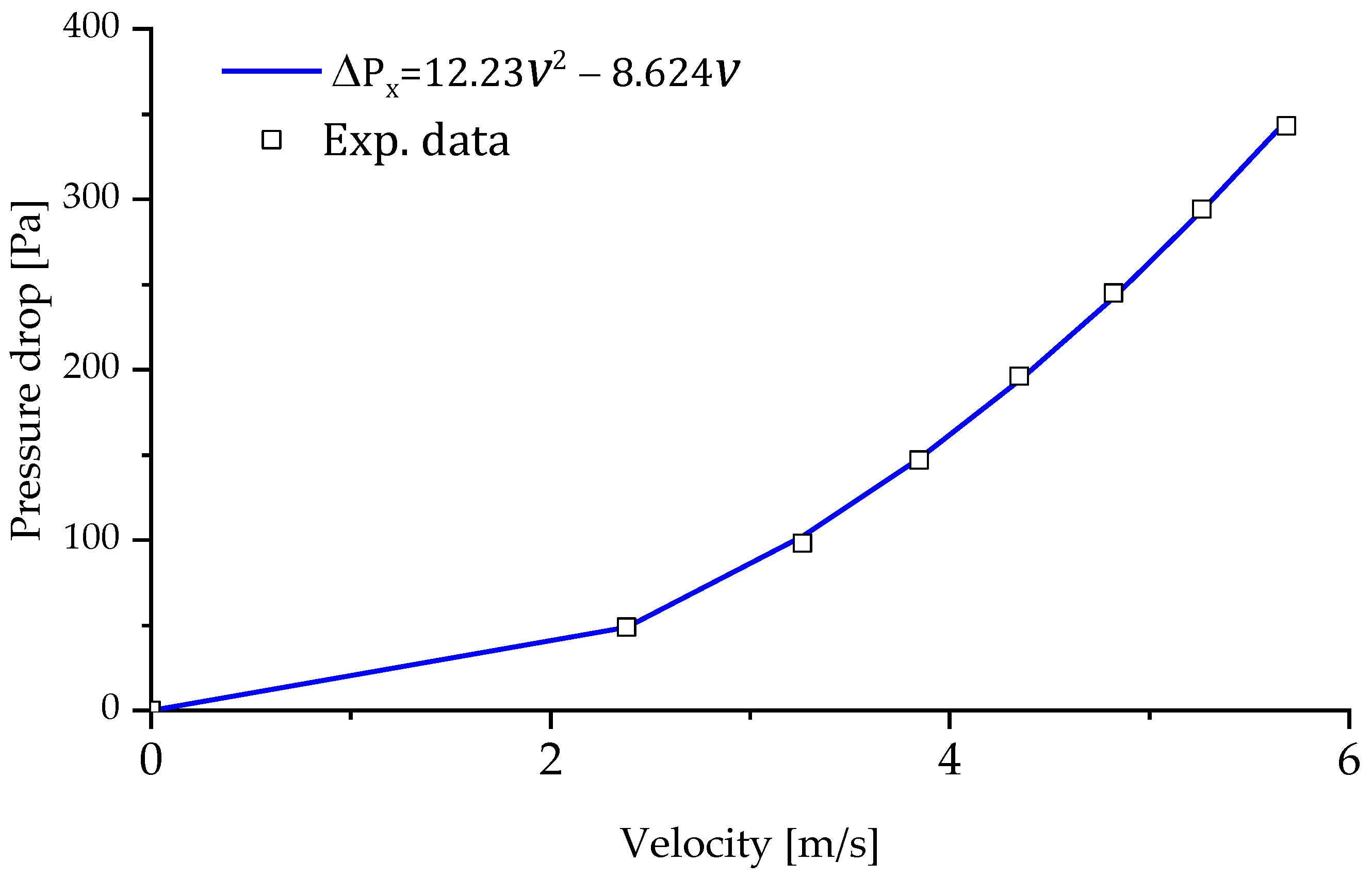
1.3. Porous Media Model for a Flame Arrestor

To ensure safety during operation, a flame arrestor is usually installed. It allows fluid to pass but prevents backfires, as well as larger fires or explosions. A flame arrestor forces the flame to pass through in only one direction and has a large contact area to remove a significant amount of heat from the flame.

Because a flame arrestor has a complex structure and thus requires an enormous number of numerical grids to resolve its detailed geometry, a porous media model, which simplifies a porous media region as a momentum sink, was applied [16]. The inertial and viscous resistance coefficients were calculated by Forchheimer as the following.

$$\Delta P=(\frac{\mu }{\alpha }V+\frac{1}{2}{C}_2\rho V^2)\Delta n$$

(3)

where $\mu$ and $\rho$ are the dynamic viscosity and density, respectively; $V$ is the magnitude of the velocity, $\Delta P=P_2-P_1$ is the pressure drop across the porous media region; $\Delta n$ is the length of the porous media region; $1/\alpha$ is the viscous loss (Darcy coefficient); and $C_2$ is the inertial resistance coefficient (Forchheimer coefficient).

2. Numerical Simulation

2.1. Geometry and Mesh

In this study, a model of VOC burner (from TEC Ltd., Ulsan, Republic of Korea) with five co-axial pipes, which was designed to ensure a large enough contact area for the fuel and gas when they are mixed, was considered. The schematic of the VOC burner is shown in Figure 2a. The position of the fuel supply inlet is marked “fuel inlet”, and it was 0.08 m in diameter. The fuel can be distributed to the 2nd and 4th axial pipes by the four connection tubes. The outside diameter of the stack is 0.6 m. Four air-inlets with a square section are in the bottom. A flame arrestor that is 0.025 m in length is installed above the burner. To prevent the high temperature of the burner from having a negative effect, insulation layers are installed inside the stack. The insulation materials have low thermal conductivity and anti-fire capability and are composed in 2 layers: Superwool^® Plus and WDS MultiFlexPlus^®. Stainless steel is used for the outside cover. The geometrical parameters of the combustor considered in this study are shown in

Table 1. Combustor parameters.

Design Model	$\mathbf{Air} \mathbf{Inlet}, {\mathit{d}}_{\mathit{a}}$$\left(\mathbf{m}\right)\times {\mathit{d}}_{\mathit{a}}\left(\mathbf{m}\right)$	$\mathbf{Stack} \mathbf{Height}, \mathit{H}\left(\mathbf{m}\right)$
M1	$0.15\times 0.15$	2.0
M2	$0.25\times 0.25$	2.0
M3	$0.15\times 0.15$	4.0

. An unstructured tetrahedral mesh was generated in Ansys ICEM-CFD software with a near-wall clustered mesh, as shown in Figure 2b.

2.2. Governing Equations

The chemical reactions involved in the gasification processes were simulated by solving the mass, momentum, and energy conservation equations and reactions for each individual species [3,7,8,10,11,12,13]. A finite volume-based commercial CFD solver, Ansys Fluent, is applied. The mass conservation for an incompressible flow was calculated, as follows [11].

$$\nabla ·(\rho \overrightarrow{u})=0$$

(4)

where $\rho$ is the species gas density; $\overrightarrow{u}$ is the velocity vector.

Similarly, the momentum conservation equation [12,13]

$$\frac{\partial (\rho \overrightarrow{u})}{\partial t}+\nabla ·(\rho \overrightarrow{u}\overrightarrow{u})=-\nabla p+\nabla ·\left(\stackrel{=}{\tau }\right)+S_i+\mathrm{g}\left(\rho -{\rho }_o\right)$$

(5)

where $p$is the pressure; t is the time; $\stackrel{=}{\tau }$ is the stress tensor; $S_i$ is source term due to porous media; and $\mathrm{g}\left(\rho -{\rho }_o\right)$ is buoyancy force due to gravity.

The total energy is obtained from the energy equation [12]:

$$\frac{\partial \left(\rho E\right)}{\partial t}+\nabla ·\left(\overrightarrow{u}\left(\rho E+p\right)\right)=\nabla ·\left({\mathsf{\lambda }}_c\nabla ·T-{\displaystyle \sum }_N{h}_i{\overrightarrow{J}}_i+\stackrel{=}{\tau }.\overrightarrow{u}-F_{h,i}\right)+{\displaystyle \sum }_N{h}_i{R}_i$$

(6)

where $E$ is the total energy; ${\mathsf{\lambda }}_c$ is the thermal conductivity; $T$ is the temperature; p is the pressure, and $h_i$ is enthalpy of species $i$; $R_i$ net rate product by chemical reaction; $F_{h,i}$ is the energy flux; $\overrightarrow{J_i}$ is the diffusion flux of species $i$ arising due to the gradient of concentration and temperature.

The species transport for the reactant and product of species $i$ was [10]:

$$\frac{\partial \left(\rho Y_i\right)}{\partial t}+\nabla · (\rho \overrightarrow{u}{Y}_i)=-\nabla · {\overrightarrow{J}}_i+R_i$$

(7)

where $Y_i$ is mass fraction (0$\le Y_i\le 1$) of each species; $R_i$ is the net rate of production by the chemical reaction. The mass diffusion fluxes in turbulent flows are:

$$\overrightarrow{J_i}=-\left(\rho D_{i,m}+\frac{{\mu }_t}{S_{Ct}}\right)\nabla Y_i-D_{T,i}\frac{\nabla T}{T}$$

(8)

where $S_{Ct}$ is the turbulent Schmidt number; ${\mu }_t$is the turbulence viscosity; and $D_{T,i }$is the thermal diffusion coefficient, $D_{i,m }$is the mass diffusion coefficient for species i. $S_{Ct}$was set to 0.7; T is the temperature.

A standard k−ε turbulent model was applied [7,10,12]. The transport equation for turbulence kinetic energy and its rate of dissipation were obtained from the following transport equations:

$$\frac{\partial }{\partial t}\left(\rho k\right)+\frac{\partial }{\partial x_i}\left(\rho k{u}_i\right)=\frac{\partial }{\partial x_i}\left[\left(\mu +\frac{{\mu }_t}{{\sigma }_k}\right)\frac{\partial k}{\partial x_i}\right]+G_k+G_b-\rho \epsilon -Y_M+S_k$$

(9)

$$\frac{\partial }{\partial t}\left(\rho \epsilon \right)+\frac{\partial }{\partial x_i}\left(\rho \epsilon u_i\right)=\frac{\partial }{\partial x_i}\left[\left(\mu +\frac{{\mu }_t}{{\sigma }_{\epsilon }}\right)\frac{\partial \epsilon }{\partial x_i}\right]+C_{1\epsilon }\frac{\epsilon }{k}\left(G_k+C_{3\epsilon }{G}_b\right)-C_{2\epsilon }\rho \frac{{\epsilon }^2}{k}+S_{\epsilon }$$

(10)

where ${\sigma }_k$ is the turbulent Prandtl number for turbulence kinetic energy; ${\sigma }_{\epsilon }$ is the turbulent Prandtl number for the turbulence dissipation rate; $G_k$ and $G_b$ represent the generation of turbulence due to mean velocity gradients and buoyance, respectively; $\mu$ is dynamic viscosity; ${\mu }_t=\rho C_{\mu }{k}^2/\epsilon$ is turbulent viscosity; and $C_{1\epsilon }$, $C_{2\epsilon }$, and $C_{3\epsilon }$ are model constants. The constants of this model are shown in

Table 2. Constant values in the k−ε model [9].

Constants	${\mathit{\sigma }}_{\mathit{k}}$	${\mathit{\sigma }}_{\mathit{\epsilon }}$	${\mathit{C}}_{1\mathit{\epsilon }}$	${\mathit{C}}_{2\mathit{\epsilon }}$	${\mathit{C}}_{\mathit{\mu }}$
Values	1.0	1.3	1.44	1.92	0.09

.

The $k-\omega$ SST model is based on the Wilcox $k-\omega$ model, in which the shear stress transport (SST) formulation switches to a $k-\epsilon$ behavior in the free stream, and it is more accurate than the standard k−ε turbulent model for the near-wall region [17]. The turbulence kinetic energy $k$ and specific dissipation rate $\omega$ were obtained from the following transport equations:

$$\frac{\partial }{\partial t}\left(\rho k\right)+\frac{\partial }{\partial x_i}\left(\rho k{u}_i\right)=\frac{\partial }{\partial x_i}\left[\left(\mu +\frac{{\mu }_t}{{\sigma }_k}\right)\frac{\partial k}{\partial x_i}\right]+G_k-Y_k+S_k$$

(11)

$$\frac{\partial }{\partial t}\left(\rho \omega \right)+\frac{\partial }{\partial x_i}\left(\rho \omega u_i\right)=\frac{\partial }{\partial x_i}\left[\left(\mu +\frac{{\mu }_t}{{\sigma }_{\omega }}\right)\frac{\partial \omega }{\partial x_i}\right]+G_{\omega }-Y_{\omega }+S_{\omega }$$

(12)

In these equations, $G_k$ represents the generation of turbulent kinetic energy due to mean velocity gradients; $G_{\omega }$ represents the generation of $\omega$; and $Y_k$ and $Y_{\omega }$ represent the dissipation of $k$ and $\omega$ due to turbulence. Turbulence viscosity is calculated using Equations (13)–(19).

$${\mu }_t=\frac{\rho k}{\omega }\frac{1}{max\left[\frac{1}{{\alpha }^{*}};\frac{S{F}_2}{a_1\omega }\right]}$$

(13)

$${\sigma }_k=\frac{1}{F_1/{\sigma }_{k,1}+\left(1-F_1\right)/{\sigma }_{k,2}}$$

(14)

$${\sigma }_{\omega }=\frac{1}{F_1/{\sigma }_{\omega ,1}+\left(1-F_1\right)/{\sigma }_{\omega ,2}}$$

(15)

$$F_1=\tan \mathrm{h}\left({\varphi }_1^4\right)$$

(16)

$${\varphi }_1=\min \left[\max \left(\frac{\sqrt{k}}{0.09\omega y};\frac{500\mu }{\rho y^2\omega }\right);\frac{4\rho k}{{\sigma }_{\omega ,2}{D}_{\omega }^{+}{y}^2}\right]$$

(17)

$$F_2=\tan \mathrm{h}\left({\varphi }_2^2\right)$$

(18)

$${\varphi }_2^2=\max \left[2\frac{\sqrt{k}}{0.09\omega y},\frac{500\mu }{\rho y^2\omega }\right]$$

(19)

$$\begin{gathered} {\alpha }^{*}={\alpha }_{\infty }^{*}=1; a_1=0.31; {\alpha }_0^{*}=0.024; {\alpha }_{\infty }^{*}=0.52; {\beta }_i=0.072; {\sigma }_{k,1}= \\ 1.176 ; {\sigma }_{k,2}=1.0; {\sigma }_{\omega ,1}=2.0; {\sigma }_{\omega ,1}=1.168 \end{gathered}$$

where y is the distance to the next surface and $D_{\omega }^{+}$ is the positive portion of the cross-diffusion term [17].

In this study, heat loss through the wall was considered using convective heat transfer with the convective heat transfer coefficient $h_f$ [11,13].

$$q=A{h}_f\left(T_w-T_f\right)$$

(20)

where $T_w$ and $T_f$ are the wall and free (ambient) temperature, respectively, and $A$ is the convection area.

When the temperature gradient in the computational domain was significant, the temperature $\left(T\right)$ effect on fluid density was calculated using Equation (21) [11,12].

$$\rho =\frac{P_{op}}{RT{{\displaystyle \sum }}_i\frac{Y_i}{M_{\omega ,i}}}$$

(21)

where $P_{op}$ is the operation pressure (atmosphere); $R$ is a universal gas constant; $M_{\omega ,i}$ is the molecular weight of species $i$; and $Y_i$ is the mass fraction of species $i$.

2.3. Validation of the Numerical Procedure

The present numerical method was validated with the combustion of methane–air reported by Brookes et al. [9]. Figure 3 shows the geometry and boundary conditions that were implemented in their experimental oxy-fuel combustor; the simplified geometry was used by Kassem et al. [7], who used the EDM and standard $k-\epsilon$ turbulent models. In this combustor, methane enters through the inner pipe, and the oxidizer is supplied through the outer pipe. The diameters of the inner and outer nozzles are 4.0 mm and 155.0 mm, respectively. Because the pipe is axisymmetric, a 2D plane computational domain with axisymmetric boundary conditions is assumed. The computational domain was discretized to 250,000 quadrilateral grid cells and the boundary conditions are shown in

Table 3. The boundary conditions.

Fuel Velocity (m/s)	${\mathit{T}}_{\mathit{C}\mathit{H}4}$ (K)	Oxidizer Velocity (m/s)	Fraction O2	${\mathit{T}}_{\mathit{O}2}$ (K)
20	290	0.5	0.23	300

. The EDM was combined with two different turbulence models, the standard k−$\epsilon$ and k−$\omega$ SST models, and results were compared with references [7,9].

The comparison of the calculated temperature with the experimental measurements is shown in Figure 4. Results are similar to those of Kassem et al. [7] and Brookes et al. [9]. The k−ω SST turbulence model produced better accuracy than the standard k−ε model, but it required more computing time and memory. The error in this study can be attributed to the neglect of the Arrhenius reaction rate; the combustion was instead assumed to be a one-step reaction controlled by the turbulence rate. Thus, the standard k−ε model in Fluent combined with the EDM might be reasonable for a turbulent combustor of CH₄ and CO.

2.4. Boundary Conditions

Simulations were performed using a transient approach with a steady solution as the initial condition. The boundary conditions for each case are shown in

Table 4. The boundary conditions.

Case	Design Model	Fuel Inlet	Air Inlet
		Fuel (CO) Mass Flow Rate (kg/h)	Pressure (Pa), Air Mass Flow Rate (kg/h)
1	M1	${\dot{m}}_f=180$	$p_{in}=0$
2	M2	${\dot{m}}_f=180$	$p_{in}=0$
3	M1	${\dot{m}}_f=180$	${\dot{m}}_{air}=720$ (by a fan)
4	M3	${\dot{m}}_f=180$	$p_{in}=0$
5	M3	${\dot{m}}_f=32$	$p_{in}=0$
6	M3	${\dot{m}}_f=54$	$p_{in}=0$
7	M3	${\dot{m}}_f=108$	$p_{in}=0$

. Specifically, Case 3 has a forced air stream of 720 kg/h, and the EA ratio was lower than 1 for the lean mixture process [5]. Here, the EA ratio is defined as the function of the stoichiometric and actual air flows, as shown by Equation (22):

$$EA=\frac{{\dot{m}}_{actual air}}{{\dot{m}}_{stoichiomtric air}}-1$$

(22)

The flame arrestor is modeled by the Forchheimer equation as a momentum sink in the momentum equation. The experiment was conducted to determine the coefficients in Equation (23). The pressure drops across the flame arrestor and the corresponding flow rates in various flow rate conditions were measured using a differential pressure gauge and a flowmeter, respectively, without chemical reaction. Figure 5 shows the experimental data and quadratic fit based on the Forchheimer equation for the velocity–pressure drop.

$$\Delta P_x=12.23V^2-8.62V$$

(23)

Compared with Equation (3), where $\rho =1.14 \mathrm{kg}/{\mathrm{m}}^3$; $\mu =1.784\times {10}^{-4}$; and $\Delta n=25 \mathrm{mm}$, it was determined that the viscous resistance factor was $1/\alpha$ = $1.9\times {10}^7$, and the inertial resistance was $C_2$ = 798. Because the effect of the porous media is valid only in the z-direction, it was set to a large arbitrary number, $1/\alpha$ = $2.0\times {10}^8$, in the x- and y-directions.

2.5. Grid Independence Test

To determine the best computational grid system a grid independence test was conducted with various mesh densities. A coarse mesh was defined as having 4 million elements; medium mesh, 8 million elements; fine mesh, 12 million elements; and an extra-fine mesh, 19 million elements. Figure 6 shows the combustion efficiency with various grid systems; here, the combustion efficiency is defined as the carbon conversion efficiency ($\eta$), as the ratio of the carbon mass flow rate in the produced CO₂ and in the fuel (CO) stream [18], as shown in Equation (24).

$$\eta =\frac{{\dot{m}}_{{\mathrm{carbon} \mathrm{in} \mathrm{produced} \mathrm{CO}}_2}}{{\dot{m}}_{\mathrm{carbon} \mathrm{in} \mathrm{fuel} \left(\mathrm{CO}\right)}}\times 100\%$$

(24)

There was a minor difference when the number of elements was higher than 8 million. To optimize the computational time and memory usage of the computer, as well as the accuracy of the data, the fine mesh was chosen as the standard for the main simulations.

3. Result and Discussion

3.1. Effect of a Flame Arrestor

The effect of a flame arrestor on flow within the fuel tubes is shown in Figure 7. The flame arrestor was modelled as a porous media region. Figure 7a depicts the significant non-uniform velocity distribution on the rings when a flame arrestor does not exist. Because the fuel is injected from the inlet on the left, higher velocity tends to occur on the right of the tubes as a result of the inertia of fluid. A relatively uniform velocity distribution forms after the fuel passes through a flame arrestor, although a slight difference between the left and right sides of the pipe remains. The comparison of velocity distribution along the axial direction of the pipes between the case without and with the flame arrestor can be seen in Figure 7b. The average velocity inside the flame arrestor (porous zone) was 2.7 m/s, corresponding to a pressure drop of 62 Pa.

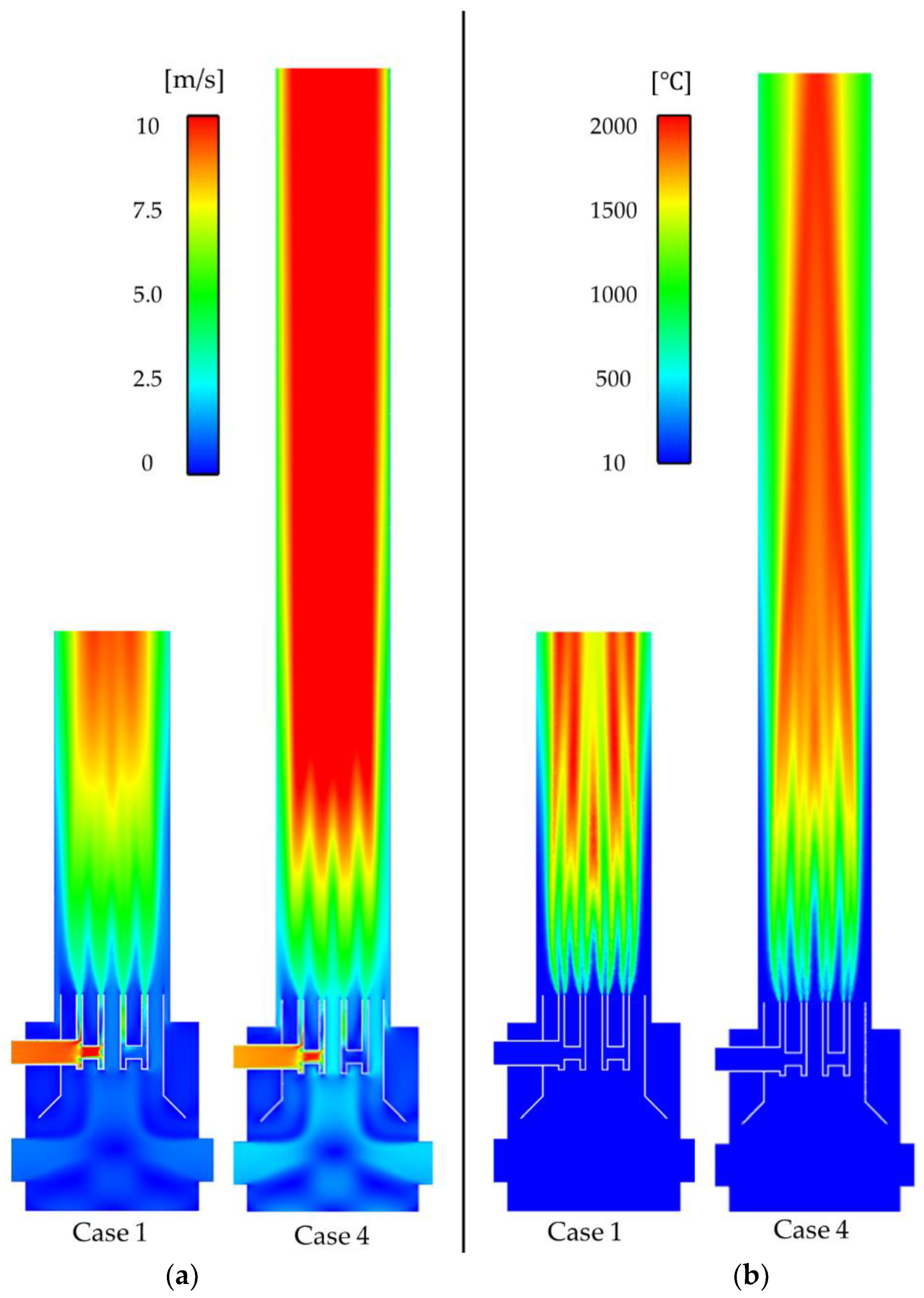
3.2. Effect of Combustor Design Parameters on the Combustion Performance

The effect of the air inlet on the efficiency of combustion was investigated. Figure 8 shows the velocity distribution on the axial plane with three different design parameters for the combustor. Case 1 had a normal-sized air inlet ($d_a$ = 0.15 m) with a square section; Case 2 had a larger air inlet ($d_a$ = 0.25 m), and Case 3 had a normal-sized air inlet with a fan. For Case 1 and Case 2, the pressure boundary condition was applied at the air inlet, whereas for Case 3, constant airflow of 720 kg/h was set to model the fan. The airflows for Case 1 and Case 2 were calculated to be 103 kg/h and 106 kg/h, respectively. The combustion efficiencies of Case 1 and Case 2 were 63% and 64%, respectively, as shown in

Table 5. Comparison of the fuel and oxygen mass flow rates and combustion efficiency.

	Case 1	Case 2	Case 3
Fuel mass flow rate, ${\dot{m}}_{fuel}$(kg/h)	180	180	180
Air mass flow rate, ${\dot{m}}_{air}$(kg/h)	103	106	720
Combustion efficiency, $\eta$ (%)	63	64	84

. Higher performance (84%) was obtained in Case 3, in which more air flows into the combustion chamber by means of a forced stream. Figure 9 shows the temperature distribution in the axial plane under various air mass flow rate conditions. The temperature was highest at the center and decreased toward the wall. The results show that the combustion efficiency depended on the air flow rate, with the size of the air inlet having only a minor effect.

The effect of the stack height on combustion efficiency was also investigated by considering stacks of 2 m and 4 m. It is known that a higher stack enhances airflow coming into the combustor by the buoyancy effect, which in turn improves the combustion performance. Figure 10 compares the velocity and temperature at different stack heights. The average velocity was 0.9 m/s for a stack of 2 m and 1.4 m/s for a stack of 4 m. The combustion performance was 63% and 94% for stack heights of 2 m and 4 m, respectively. Thus, the combustion performance was enhanced by 50% when the stack height increased from 2 m to 4 m. This agrees with stack effect that was described in reference [2]. In particular, it was observed that most of the airflow entered the combustor through the center pipe because the horizontal connecting tubes hindered the flow of air to the other surrounding pipes.

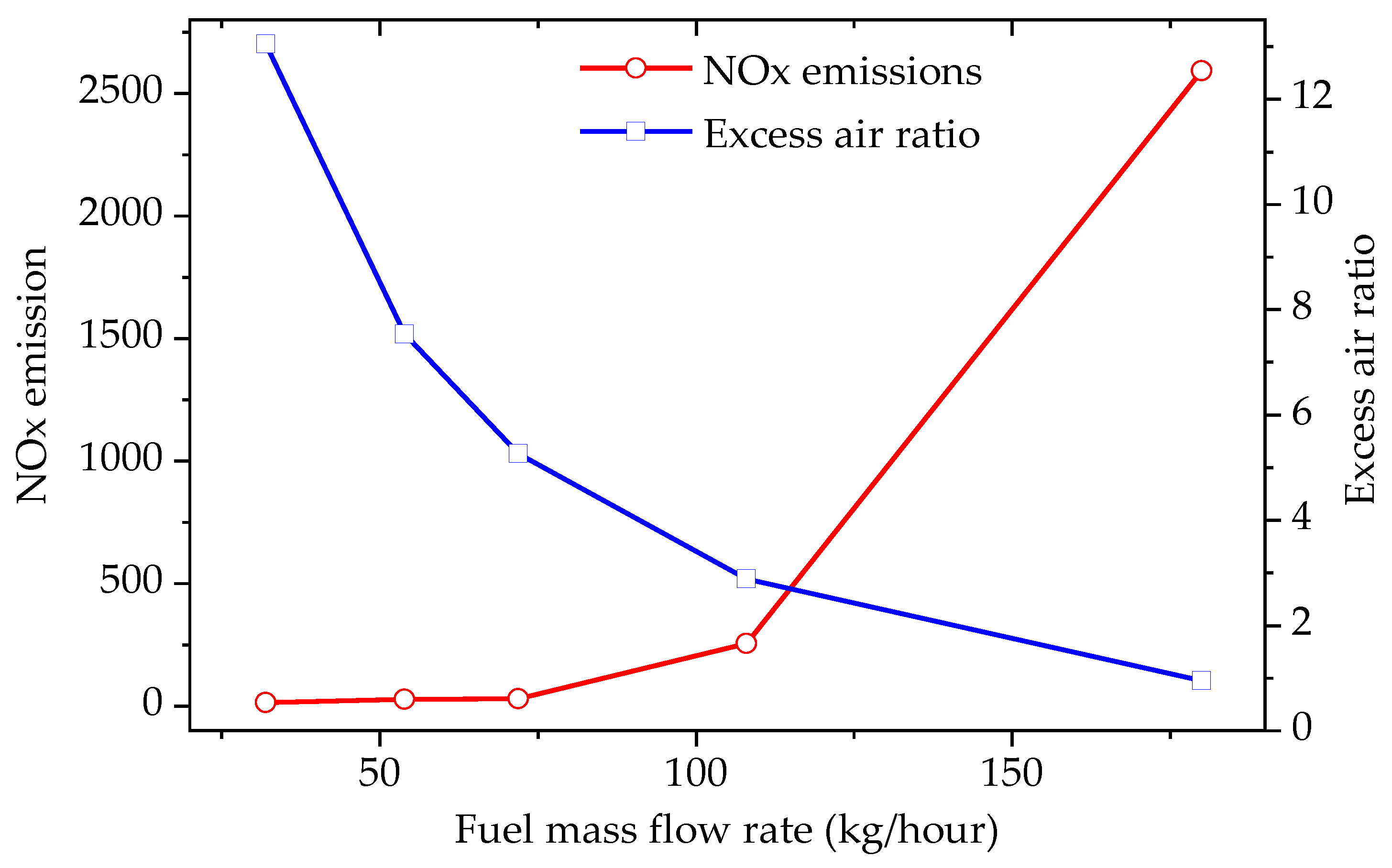
3.3. Effect of the Fuel Mass Flow Rate (FMR) on Combustion Performance

Figure 11 shows the EA ratio as a function of the FMR. A lower FMR produces a higher EA ratio, and vice versa. Thirteen times more air, relative to stoichiometric air, was present when the FMR was 32 kg/h. The EA ratio was 1.1 at the maximum FMR with complete combustion (Case 4). A higher EA number is more efficient, but it causes a higher level of NOx emissions, as shown in Figure 12. The relationship of EA ratio and NOx emissions with fuel mass flow rate showed a similar trend to that in the previous study [3,5]. The FMR must be less than 180 kg/h for complete combustion.

As plotted in Figure 13, it was observed that the temperature was symmetrically distributed along the center line of the stack, which prevented direct flame from affecting the insulation material on the stack wall. As the fuel mass flow rate increased, the outlet temperature also increased gradually due to an increase in the volume flow rate of the air, which led to an increase in the heat generated by the reactions. The maximum temperature was near the central region and tended to decrease gradually toward the near-wall regions. The maximum temperature at the inner walls did not exceed 1450 °C, as shown in Figure 13, which satisfied the conditions required by these materials.

4. Conclusions

The conjugate heat transfer analyses of the process of combusting VOCs and heat transfer in the insulated wall layer were conducted by using a standard $k-\epsilon$ turbulence model and the EDM for chemical reaction modeling. Based on the numerical simulations, detailed thermal fluid flow characteristics of natural and forced combustion in a VOC burner with the effect of a flame arrestor were obtained.

Results showed that the size of the air inlet had only a minor effect on combustion efficiency and that the airstream forced by a fan significantly enhanced the combustion performance. In particular, increasing the height of the stack from 2 m to 4 m greatly increased combustion efficiency from 63% to 94%, with a 50% increase in the incoming air flow rate by natural convection, which emphasizes the importance of stack height in combustor design. In addition, from the heat conduction analysis for the stack wall, the heat insulation system of the considered model has been shown to effectively prevent heat transfer to the outer wall surface. Further detailed parametric studies for different configurations of VOC burner will be necessary.

References

1. Muir, B.; Sobczyk, M.; Bajda, T. Fundamental features of mesoporous functional materials influencing the efficiency of removal of VOCs from aqueous system. Sci. Total Environ. 2021, 784, 147121. [Google Scholar] [CrossRef] [PubMed]
2. Das, P.; Chandramohan, V.P. Effect of chimney height and collector roof angle on flow parameters of solar updraft tower (SUT) plant. J. Therm. Anal. Calorim. 2019, 136, 133–145. [Google Scholar] [CrossRef]
3. Pundle, A.; Sullivan, B.; Means, P.; Posner, J.D.; Kramlich, J.C. Predicting and analyzing the performance of biomass-burning natural draft rocket cookstoves using computational fluid dynamics. Biomass Bioenergy 2019, 131, 105402. [Google Scholar] [CrossRef]
4. Lee, C.C.; Tran, M.V.; Nurmukan, D.; Tan, B.T.; Chong, C.T.; Scribano, G. Investigation of flame and stabilization characteristics of palm-methyl-esters diffusion flames. Fuel 2022, 313, 123034. [Google Scholar] [CrossRef]
5. Qian, X.; Lee, S.; Chandrasekaran, R.; Yang, Y.; Caballes, M.; Alamu, O.; Chen, G. Electricity evaluation and emission characteristics of poultry litter co-combustion process. Appl. Sci. 2019, 9, 4416. [Google Scholar] [CrossRef] [Green Version]
6. Al-Arkawazi, S.A.F. Analyzing and predicting the relation between air–fuel ratio (AFR), lambda (λ) and the exhaust emissions percentages and values of gasoline-fueled vehicles using versatile and portable emissions measurement system tool. SN Appl. Sci. 2019, 1, 1370. [Google Scholar] [CrossRef] [Green Version]
7. Kassem, H.I.; Sqar, K.M.; Aly, H.S.; Sies, M.M.; Wahid, M.A. Implementation of the eddy dissipation model of turbulent non-premixed combustion in OpenFoam. Int. Commun. Heat Mass Transf. 2011, 38, 363–367. [Google Scholar] [CrossRef]
8. Murugan, P.C.; Prasad, G.A.; Sekhar, S.J. Implementation of species-transport model in numerical simulation to predict the performance of downdraft gasifier with biomass blends. Energy Res. J. 2019, 10, 36–47. [Google Scholar]
9. Brookes, S.J.; Moss, B.J. Measurements of soot and thermal radiation from confined turbulent jet diffusion flames of methane. Combust. Flame 1999, 116, 49–61. [Google Scholar] [CrossRef]
10. Yilmaz, H.; Cam, O.; Tangoz, O.; Yimaz, I. Effect of different turbulence models on combustion and emission characteristics of hydrogen/air flames. Int. J. Hydrog. Energy 2017, 42, 25744–25755. [Google Scholar] [CrossRef]
11. Jiaqiang, E. Numerical investigation on hydrogen/air non-premixed combustion in a three-dimensional micro combustor. Energy Convers. Manag. 2016, 134, 427–438. [Google Scholar]
12. Halouane, H.; Dehbi, A. CFD simulations of premixed hydrogen combustion using the Eddy Dissipation and the Turbulent Flame Closure models. Int. J. Hydrogen Energy 2017, 42, 21990–22004. [Google Scholar] [CrossRef]
13. Yilmaz, H.; Kareyen, S.; Tepe, A.U.; Bruggemann, D. Colorless distributed combustion characteristics of hydrogen/air mixtures in a micro combustor. Fuel 2022, 332, 126163. [Google Scholar] [CrossRef]
14. Zhen, H.S.; Wei, Z.L.; Liu, Z.H.; Wang, X.C.; Huang, Z.H.; Leung, C.W. A state-of-the-art review of lab-scale inverse diffusion burners & flames: Form laminar to turbulent. Fuel Process. Technol. 2021, 222, 106940. [Google Scholar]
15. Artemov, V.; Beale, S.B.; de Vahl Davis, G.; Escudier, M.P.; Fueyo, N.; Launder, B.E.; Leonardi, E.; Malin, M.R.; Minkowycz, W.J.; Patankar, S.V.; et al. A tribute to D.B. Spalding and his contributions in science and engineering. Int. J. Heat Mass Transf. 2009, 52, 3884–3905. [Google Scholar] [CrossRef] [Green Version]
16. Farah, H.D. Numerical Study of Detonation Flame Arrestor Performance and Detonation Interaction with the Arrestor Element. Ph.D. Thesis, The University of Texas at Arlington, Arlington, TX, USA, 2019. [Google Scholar]
17. Menter, F.R. Two-equation eddy-viscosity turbulence models for engineering applications. AIAA J. 1994, 32, 1598–1605. [Google Scholar] [CrossRef] [Green Version]
18. Burtt, D.C.; Corbin, D.J.; Armitage, J.R.; Crosland, B.M.; Jefferson, A.M.; Kopp, G.A.; Kostiuk, L.W.; Johnson, M.R. A methodology for quantifying combustion efficiencies and species emission rates of flares subjected to crosswind. J. Energy Inst. 2022, 104, 124–132. [Google Scholar] [CrossRef]
Figure 1. The types of burner (a) non-premixed; (b) premixed; (c) partial premixed.
Energies 16 00170 g001
Figure 2. (a) Schematic of the VOC burner; (b) computational grid system for the VOC burner.
Energies 16 00170 g002
Figure 3. Schematic diagram of the furnace of experiment [7].
Energies 16 00170 g003
Figure 4. Temperature profiles at the height of (a) h = 0.15 m; (b) h = 0.30 mm; and (c) along the axial direction [7,9].
Energies 16 00170 g004
Figure 5. Relationship between pressure drops and velocity in the flame arrestor.
Energies 16 00170 g005
Figure 6. Grid independence test with different numbers of elements.
Energies 16 00170 g006
Figure 7. Effect of a flame arrestor on the velocity distribution: (a) isoview, (b) axial plane.
Energies 16 00170 g007
Figure 8. Comparison of the velocity distribution in the axial plane in different air inlet conditions (y = 0).
Energies 16 00170 g008
Figure 9. Comparison of temperature contours in the axial plane under different airflow conditions.
Energies 16 00170 g009
Figure 10. Comparison of the velocity and temperature distributions in the axial plane at different stack heights: (a) velocity, (b) temperature.
Energies 16 00170 g010
Figure 11. Excess air ratio and efficiency at different fuel mass flow rates.
Energies 16 00170 g011
Figure 12. NOx emission and excess air ratio at different fuel mass flow rates (z = 3 m).
Energies 16 00170 g012
Figure 13. Comparison of temperature profiles at the axial position of z = 3.5 m with different FMRs.
Energies 16 00170 g013