Article

Research on Production Profiling Interpretation Technology Based on Microbial DNA Sequencing Diagnostics of Unconventional Reservoirs

1
School of Energy Resources, China University of Geosciences (Beijing), Beijing 100190, China
2
School of Petroleum Engineering, China University of Petroleum (Beijing), Beijing 102249, China
3
Geology Research Institute, Greatwall Drilling Company, China National Petroleum Corporation (CNPC), Beijing 100101, China
4
The Second Gas Production Plant of PetroChina Changqing Oilfield Company, Yulin 719000, China
*
Author to whom correspondence should be addressed.
Energies 2023, 16(1), 358; https://doi.org/10.3390/en16010358
Submission received: 31 October 2022 / Revised: 21 December 2022 / Accepted: 26 December 2022 / Published: 28 December 2022

Abstract

:
Production profiling technology is an important method for monitoring the dynamics of oil and gas reservoirs which can effectively improve the efficiency of oil recovery. Production profiling is a technique in which a test instrument is lowered from the tubing to the bottom of the well to measure flow, temperature, pressure, and density in a multi-layer section of a producing well. Normal production profiling process needs to stop production, operate complex, consume long time and high cost. Furthermore, the profile cannot be continuously monitored for a long time. To address these limitations, this paper proposes a production profiling interpretation method based on reservoir primitive microbial DNA sequencing. The microbial stratigraphic baseline with high-resolution features is obtained by sampling and DNA sequencing of produced fluid and cuttings from different wells. Specifically, the random forest algorithm is preferred and improved by comparing the accuracy, precision, recall, F1-score, and running time of three clustering methods: Naïve-Bayes classifier, random forest classifier, and back-propagation classifier. Constructing PSO-random forest model is based on stratigraphic records and produced fluid bacteria features. The computational accuracy and efficiency of this method allows it to describe the production profile for each formation. Moreover, this test process does not need to stop production with simple operation and does not pollute the formation. Meanwhile, by sampling fluid production at different stages, it can achieve the purpose of long-term effective dynamic monitoring of the reservoir.

1. Introduction

Rapid economic development has greatly increased the demand for petroleum resources, which in turn has contributed to the development of the oil exploration business. The exploration and exploitation of oil fields is directly related to the quality of oil business development and has a direct impact on economic security. Production profiling technology is one of the most critical technical tools in the current oil exploration industry, which directly affects the quality and efficiency of oil recovery. This paper provides an in-depth analysis of the production profiling technology and interpretation methods.
Production profiling technology is indispensable to the production logging process. At present, mature production profiling technology is to use cables, continuous tubing, and crawlers to transport the production profiling instruments through the oil jacket annulus to the injection section. At the same time, turbine flow meters and water-holding rate meters are used to monitor the flow and water content in real time. However, normal fluid production profiling tests in horizontal wells face problems such as multi-phase fluid stratification in the horizontal section and the inability to lower the cable. 2011, Lv Yiming used instrumented test tools such as MAPS array loggers and crawlers for fluid production profiling tests, but it was difficult to access the well and costs high [1]. 2021, Di Dejia proposed the fiber optic temperature and pressure testing method, which could not monitor for a long time. This technology is expensive and shows great difficulty in construction and data interpretation. Therefore, the technology needs further improvement [2]. In 2021, Qing Chang proposed the method of using substance tracer for production profiling, and selected elements with very small content in the formation fluid as markers to analyze the fluid production in each section [3]. In 2016, P.F. Yue proposed the swabbing fluid production profiling technique, which was to extend the swab tubular into downhole instead of the original production tubular to obtain the well production [4]. This production profiling technique required little well slope, but the operation time was long and the strong pumping led to a lower accuracy as it did not reflect the real situation of reservoir fluid production (S.B. Du et al., 2018) [5]. In 2008, H.Z. Cui proposed the annular production profiling technique, which was more commonly used in the later stages of oilfield development. This technique involved a small-diameter tester that was lowered into the formation from a test hole at the eccentric wellhead and fused with static data to achieve a dynamic monitoring effect [6]. The annular type required a relatively large well slope, less than 20° above the pump hang. The test was carried out under normal production of the well and the results could reflect the fluid production of the reservoir (S. B. Du et al., 2018) [5]. In 2016, D.Q. Qin proposed the pre-set production profiling technique, which used a crawler to transport the downhole instrument to the measurement well section and combined it with the test instrument to achieve the production profiling purpose [7]. The pre-set had no requirement for well slope and could accurately reflect the reservoir fluid production, but the operation time was long and the production investment was high [5]. In summary, the normal production profiling technology had disadvantages such as the need to stop production during operation, complicated and time-consuming operational steps. Moreover, these techniques commonly cost high and could not be continuously monitored for a long time. With the increasingly widespread application of microbial gene sequencing technology within the petroleum area, this paper proposes a production profiling technique based on microbial DNA sequencing, which can address the above problems.
Modern civilization compares oil to the “blood of the earth”. In health testing, we often draw blood for genetic testing to find out the relevant genes and factors that lead to the occurrence of a disease. Moreover, we often provide targeted treatment for these conditions. Similarly, genetic sequencing of petroleum microorganisms allows us to monitor reservoir production dynamics in a timely manner and to obtain the production profiling at different stages in real time, thus providing an important basis for reservoir production plan adjustment (Figure 1).
Microbial gene sequencing technology has been widely used in the petroleum field for a long time. In 1984, E. Y. Chen proposed the use of microbial DNA sequencing to determine the location and extent of microbial corrosion on pipelines [8]. In 2021, Y.P. Tang proposed to find oil and gas enrichment zones by analyzing the development level of microorganisms that feed on light hydrocarbons [9]. In 1947, Zobell proposed microbial enhanced recovery (MEOR) technique for tertiary oil recovery. This technique had the advantages of low cost, environmental protection, and extended reservoir life [10]. Microorganisms are able to survive under reservoir temperatures and pressures. Therefore, microorganisms are pervasive in the subsurface and are present in primary and secondary pores, fractures, and faults. In 2020, Jordan Sawadogo compared DNA sequencing results of produced fluids sampled from different wellheads and concluded that the higher the similarity of sequencing results, the stronger the inter-well connectivity [11]. In 2019, Michael Hale used the production profiling constructed from cuttings and produced fluid DNA sequencing results to determine the formation with higher contribution to produced fluid. More specifically, a method to determine the range of minimum and maximum fracture extension height after fracturing was proposed [12]. In 2020, Mathias Schlecht determined the effect of completion sequence on the degree of fracture extension, inter-well connectivity, and the effect of proppant loading intensity on fracture extension with the produced fluid DNA sequencing results [13]. In 2019, Michael Hale demonstrated that this technique could distinguish fracture fluids from formation fluids by determining the effect of microbial DNA sequencing results on early fluid production [14]. In 2019, Elizabeth Dennet obtained the most productive formation fluids by sequencing the produced fluids and comparing the results with those obtained by traditional tracer methods, the conclusions were consistent [12]. As of 2018, DNA sequencing technology has been applied to more than 200 wells in eight basins in the Northern America, including the Permian Basin, Eagle Ford, and Bakken Shale zones. Subsurface DNA diagnostics were used to evaluate inter-well communication, calculate oil reserves, and establish production profiling. Formation communication could also be determined based on fluid-producing microbial DNA information to maximize reservoir optimization, such as well spacing and completion design (Silva, J, 2018) [15]. In 2020, Zhang Yuran conducted a 10-month-long multi-point monitoring of microbial in a network of hydraulic-conducting fractures in a gold mine tunnel 1500 m deep from the surface in South Dakota, USA. The longest sustained and highest resolution data on the microbial community of the deep fracture aquifer were obtained to date. This data validated the diversity of microbial communities in deep ground, with distinct microbial community distributions in different fractures within the same formation. This verified that the resolution of DNA sequences was sufficiently high in dimensionality and sensitivity to distinguish between localized areas of the same geological formation, while the geochemistry of two fractures was almost identical [16]. In 2022, Zhang Yuran obtained the relative abundance of microbial community in fracture fluids and its change over time through a new generation of high-throughput sequencing technology. It was verified that although the composition of deep microbial community was extremely stable most of the time, the microbial community has changed rapidly and substantially at several time points. The microbial community of different production wells has significant correlation across time and space [17]. Taken together, deep-ground microbial DNA sequencing results have been shown to have sufficiently high-resolution characteristics to be applied in fluid-producing profiling techniques.
Therefore, the goal of this study is to construct a reservoir microbial DNA sequence-based production profiling interpretation method for tracing the dynamic behavior of reservoir fluids. Through sampling and cryogenic transportation of the produced fluids and cuttings from different wells, laboratory processing, and DNA sequencing, the baseline indicates that the characteristics of formations constructed and the produced fluids are stratigraphically traced. The existing mainstream microbial traceability methods include Source Tracker based on Bayesian algorithm and FEAST based on expectation maximization algorithm [18,19]. However, the accuracy of these methods is low, and the method of increasing the accuracy by the number of iterations obviously leads to an increase in running time. Moreover, the construction of a production profiling does not require the traceability for each formation individually. Therefore, this paper proposes a production fluids traceability algorithm. By comparing the production fluids traceability accuracy of three clustering methods such as Naïve Bayesian, back propagation, and random forest, it was found that random forest is preferred. The improved PSO-random forest clustering algorithm can accurately describe the production fluids profiles. The production profiling method is a non-invasive technique, which does not need to stop the operation. By sampling and tracing the produced fluid at different stages, the purpose of long-term and effective dynamic monitoring of the reservoir can be achieved.
Under the current international situation, it is necessary for petroleum resources and shallow geothermal resources to coexist, so as to meet the global energy demands. Reasonable development and utilization of shallow geothermal resources to achieve clean heating is an effective solution to alleviate the pressure on resources and environment caused by excessive dependence on fossil energy heating. Therefore, the design of borehole heat exchangers (BHE) and simulation of the grout material impact of borehole heat exchangers in aquifers are particularly important [20]. The presence of the borehole filling material does not significantly influence either the energy exchange or the temperature profile in the aquifer. Consistent with the viewpoint in this paper, shallow geothermal resources can also realize long-term regeneration and recycling.

2. Methods

This paper focuses on the establishment of the production profiling through sample preparation, DNA sequencing and data processing, traceability of establishment of produced fluids, and produced fluid profiles. DNA sequencing are performed on cuttings and produced fluids samples from two straight and horizontal wells. The process of cuttings and produced fluids samples preparation includes DNA extraction and PCR amplification. The DNA sequencing results are processed to filter the data for downstream analysis to establish the stratigraphic baseline. Based on the three methods of Naive Bayes, random forest, and back propagation, the stratigraphic formations are clustered. The random forest algorithm is optimized and improved to efficiently and accurately trace the stratigraphic origin of the produced fluid, so as to construct the production profiling and monitor the fracture extension height after fracturing in real time. The main method flow of this paper is shown in the Figure 2. Through the above methods, this paper aims to propose a production profiling interpretation method based on reservoir primitive microbial DNA sequencing.

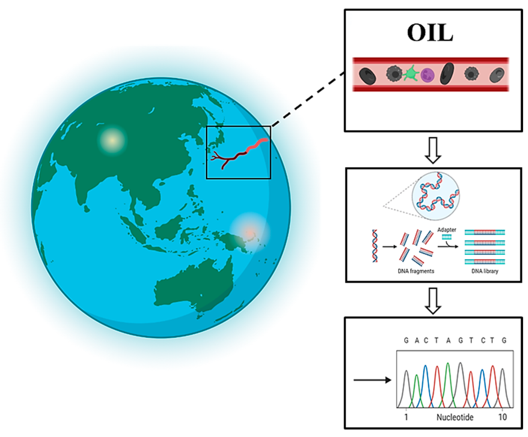
2.1. Sample Preparation

Block X is a relatively simple structure, longitudinally including ten small layers with a wide distribution area and a single layer thickness of about 20 m. The core of the main area has an average porosity of 29.4% and an average permeability of 74.5 × 10⁻³ μm2, which belongs to a high-porosity medium-low permeability reservoir. The reservoir microbial community data with high resolution are obtained by sampling cuttings as well as up to 5 months of produced fluids.
Cuttings are usually sampled from the shaker at the wellhead. Samples are collected every 3–4 m in straight wells and every 10 m in horizontal wells. The sampling process does not require the deployment of downhole tools, sample collection does not cause rig downtime. The process is non-polluting and non-destructive to the formation background concentration. Sampling of produced fluids is performed every 15 days. Produced fluids are collected directly from the wellhead, and liquid samples are collected in sterile conical flasks, each container containing 30 mL and cooled immediately after sampling to reduce microbial bloom, with cooling temperatures near −80 °C [21]. Finally, the cuttings and produced fluids samples are quickly transported to the laboratory.

2.1.1. Sample Pretreatment

The cuttings in the laboratory are size-sorted, and those with diameters of 1~3 cm are retained, cleaned, and ground to a fine powder, and then collected into conical flasks. About 10~50 g of cuttings fine powder is added to the centrifuge tube, and 100 μL of cleaning buffer was added to make a solution; then one percent of the solution volume of sodium dodecyl sulfate was added to the solution and mixed well to get the buffer solution (adjust the pH of the buffer solution to 7.5, then add 10 times the volume of distilled water of the buffer solution and mix well) [22]. The bacterial solution was concentrated by filtration with a filter membrane. Then the mixture was centrifuged at 12,000 rpm/min for 15 min. The bacterial precipitate after centrifugation is frozen to −80 °C and stored until extracted.

2.1.2. DNA Extraction

Microbial DNA is extracted from cuttings and produced fluids samples respectively. First, 82 mL of DNA extraction buffer, 0.5 mL of 6% sodium pyrophosphate, and 30 g of 0.1 mm zirconium beans were added to the bear beater container, and mixed well and heated. Then the samples were transferred to a centrifuge tube, and lysozyme, 340 μL protease K (Merck, 20 mg/mL), 3.4 mL 20% SDS were added and incubated in a water bath at 62 °C for 45 min. About 10 μL of LPA (2–4 m/μL) was added andmixed well. Then, 0.04 times the volume of 5 M sodium chloride and 0.7 equal volume of isopropanol were added. The samples were incubated on ice and then centrifuged to collect the supernatant. One volume of phenol: imitation: isoamyl alcohol was added and the sample was repeatedly centrifuged to extract purified DNA.

2.1.3. PCR Amplification

The purpose of PCR amplification is to achieve DNA replication of low biomass sample organisms in vitro, thereby significantly increasing the amount of trace DNA. PCR amplification of 16S ribosomal RNA gene can be carried out from most new bacteria using primers, and highly conservative sequences between primers and bacterial species are annealed [23]. Using Veriti, pre-denature for 25 cycles for 5 min at 93 °C, denature for 30 s, anneal for 40 s at 55 °C, and extend for 1 min at 72 °C.

2.2. DNA Sequencing and Data Processing

2.2.1. DNA Sequencing

During sequencing, the DNA strands bind to the surface of the enclosed cells and replicate the scaffold as in PCR. After sequencing, the DNA sequence data can be converted to readable text and the raw sequence data are stored in the database and associated with the original sample metadata. For sequencing results, the reads are spliced into Tags by Overlap relationships between reads. The Tags are clustered into bacteria at a given degree of similarity, and the bacteria are then annotated with species by comparing them with the database to determine the types of bacteria and their abundance.

2.2.2. Downstream Data Filtering

Figure 3 represents the accuracy of DNA sequencing results at different sample amounts and biomass. It can be seen that the accuracy of DNA sequencing results is higher when the number of samples is higher and the biomass is higher. This is due to the fact that when the sample number and biomass are higher, the DNA sequences contaminated by environmental and other factors have less influence on the data accuracy and the DNA sequencing results are more accurate. Since the biomass of cuttings microorganisms is low, it is more difficult to extract DNA from the samples. DNA sequences contaminated by environment account for a larger proportion of the DNA sequences, which have a greater impact on the accuracy of the subsequent analysis results, so a strict quality control process is designed to ensure the accuracy of downstream analysis.
First set negative control experiment before DNA extraction, the community is diluted with microbial free water for eight rounds of consecutive three-fold. With the increase of dilution, the sample microbial sequence gradually reduced, after which the sequenced DNA marker is the laboratory reagent contaminant sequence.
Define downstream analytical mass fraction, which means the number of actual DNA sequences of the sample as a percentage of the number of all DNA sequences measured, i.e., the DNA sequences with laboratory contaminating reagents removed as a percentage of the number of all DNA sequences obtained by sequencing, denoted as:
D o w n s t r e a m   a n a l y s i s   m a s s   f r a c t i o n = ( 1 Number   of   contaminated   DNA   sequences Total   sample   DNA   sequences ) × 100 %
Figure 4 shows that 86% of the sample data are available for further downstream analysis. All data are divided into three parts according to the 80% threshold and total biomass (number of DNA sequences per sample), where the yellow area with downstream analysis mass fraction less than 0.8 and also lower biomass is invalid area, which cannot be used for further sequencing analysis due to low downstream analysis mass fraction. The sequencing data with downstream analysis mass fraction above 0.8 are mainly concentrated in the range of biomass 5~30. The blue area meets both the medium biomass and downstream analysis mass fraction above 0.8, so it can be used for downstream analysis. The sequencing data in the biomass greater than 30 region are considered to be caused by microbial overgrowth, so the sequencing data in the purple region also cannot be used for downstream analysis; the data in the valid region that can be used for downstream analysis after quality control are shown in the blue region in Figure 4.

2.3. Traceability of Produced Fluids

2.3.1. Produced Fluids Traceability Model

This model assumes that all pollution sources have been eliminated from the above downstream data filtering process, and all sequencing results are obtained from the bacteria of cuttings and produced fluids. At the same time, this model assumes that bacteria do not propagate further from the deep ground to the surface, the sequencing results can completely reflect the underground situation. More specifically, all formations characteristic data do not consider human interaction factors. It is assumed that the correlation error of variables in the prediction model is within an acceptable range.
Clustering is a process of classifying data into different classes, so objects in the same cluster have great similarity, while objects between different clusters have great dissimilarity. Since this paper aims to explore the probability that the production fluid originates from each formation, the data training set has been assigned labels, and the output variables are discrete, so it is a classification problem. The classification problem is predicted by constructing a model to discover new layers based on the existing feature information for the attributes of the features to be classified. As shown in Figure 5, the input data required to build the liquid-producing formation traceability model include the baseline data of formations obtained from DNA sequencing of cuttings microorganisms, which means the bacteria and their abundance in each formation. The data are obtained from DNA sequencing of cuttings in two straight wells and two horizontal wells. The output is the probability that the produced fluid originates from each formation, which means the contribution of each formation to the produced fluid.
There are many types of common classification algorithms, among which the back propagation approach to classify data sets is achieved by simulating the behavior of the human brain, i.e., building a mesh model similar to synaptic connections. And association rule-based classification uses a heuristic approach to select the best rule for classification, which is required to satisfy specific conditions.
Bayesian classification algorithm uses Bayesian principle to calculate the probability size of samples to be classified belonging to different classes for selecting the class to which the samples belong. The support vector machine algorithm classifies sample points in a dataset by constructing a hyperplane that satisfies the minimum distance between two sample points of different categories separated by the closest distance to this plane on either side of the plane. The random forest method randomly samples the sample observations and feature variables of the dataset separately, and the result of each sampling is a tree, and each tree generates rules and classification results that match its own attributes, and the forest finally integrates the rules and classification results of all decision trees. Due to the characteristics of the data set in this paper and the characteristics of the classification algorithms studied, the model performance of three classification algorithms, back propagation, Naive Bayes, and random forest, is investigated in this paper.

2.3.2. Clustering Method Optimization

Sample data interpretation and clustering model is shown in Figure 6.
The specific analysis process is shown below.
(1)
Data standardization;
In order to avoid the influence of the scale on the variable data, the data should be standardized first. The normalization treatment used in this paper is Range0tol (graded regular transformation/specified transformation), where the transformed data have a minimum of 0 and a maximum of 1, and the rest are in the interval [0, 1] with a graded dimensionless difference of 1.
(2)
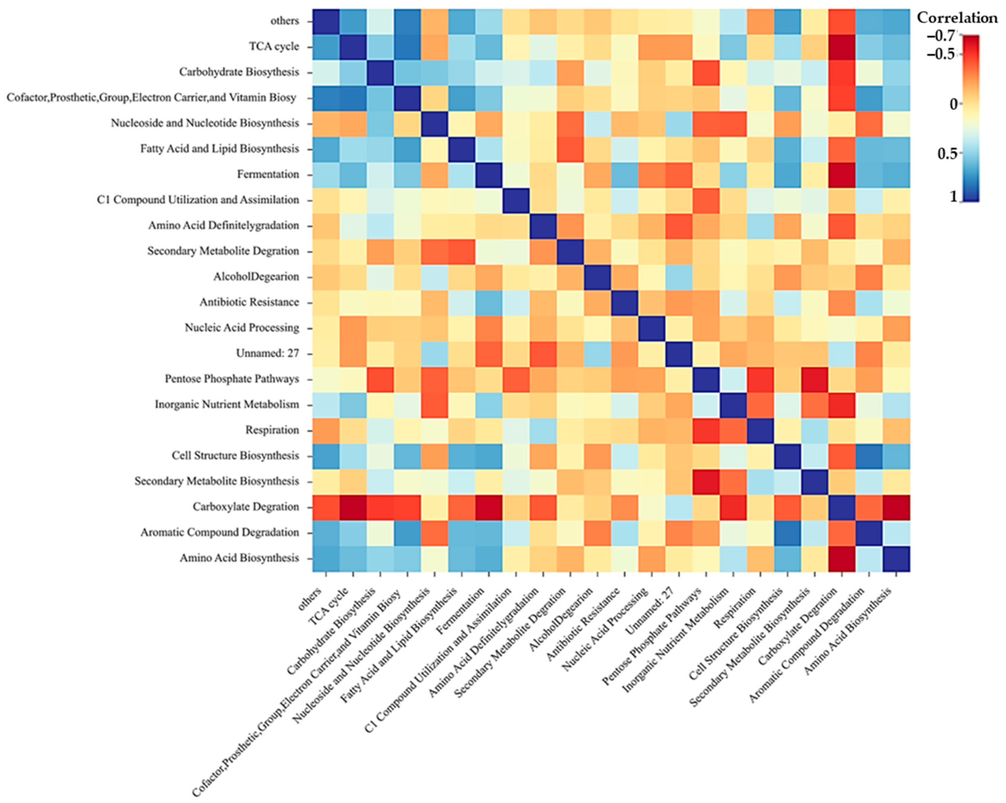
Correlation analysis;
Correlation is a measure of the relevance of data attributes, and the correlation coefficient can be used to measure the degree of correlation between two things. In this paper, Pearson coefficient is used to determine the degree of correlation between different formations of bacteria. As shown in Figure 7, according to Pearson correlation analysis, the following correlation heat map can be obtained.
(3)
Clustering method selection;
The clustering method used in this paper is shown below, and the specific steps are detailed in the Appendix A.
  • Naive Bayes classification;
It is a series of simple probabilistic classifiers based on the application of Bayes’ theorem under the assumption of strong independence between features. Using different formations and their abundance as variables, a Naive Bayes classifier capable of distinguishing different formation is generated, and the network diagram is shown in Figure 8a.
  • Random forest classification method;
Random forest classification in the process of generating many decision trees, by randomly sampling the sample observations and feature variables of the data set respectively, each sampling result is a tree, and each tree will generate rules and classification results that match its own properties, and the forest finally integrates the rules and classification results of all decision trees to achieve the classification of the random forest algorithm. The network diagram is shown in Figure 8b.
  • Back Propagation classification method;
Back propagation is a multilayer feedforward network trained by error backpropagation algorithm, which is one of the most widely used back propagation models. As shown in Figure 9, the learning rule of back propagation is to use the most rapid descent method to continuously adjust the weights and thresholds of the network by backpropagation to minimize the classification error rate of the network.
(4)
Production profiling traceability algorithm preferences Method;
First, evaluate the parameter sensitivity of each method. The sensitivity of each algorithm parameter is compared with the weight of each factor for algorithm optimization. In order to compare the model performance of the three classification methods, the preferred algorithm of the production profiling traceability algorithm is obtained by comparing the five evaluation indexes accuracy, precision, recall, F1-score, and running time of the three clustering methods respectively. Accuracy indicates the proportion of the total number of samples with the same actual source of produced fluid and the predicted source of produced fluid to the predicted source of produced fluid in the formation. Precision indicates the proportion of the number of samples that are actually 1 out of the number of all samples with a predicted result of 1. Recall is the proportion of the total number of samples with the same actual source and predicted source to the actual source. ROC curve, called receiver operating characteristic curve, reflects the trend of true positive rate (TPR) with false positive rate (FPR). It is a curve plotted with the true positive rate (sensitivity) as the vertical coordinate and the false positive rate (1-specificity) as the horizontal coordinate.

2.3.3. Improvement of Clustering Method

Random forest is a combined classification method of ensemble learning. As an important machine learning algorithm, stochastic forest algorithm is generally applicable to most data sets. By using PSO algorithm to optimize and weight leaf nodes, the performance of traditional random forest algorithm can be improved and its classification ability can be improved. Taking advantage of PSO algorithm’s strong global search ability and fast convergence speed, the random forest is improved. As a combination method of classifiers, the randomization of the random forest algorithm in the selection of training data sets and eigenvalues can effectively avoid the disadvantage of over fitting decision trees, and enhance the generalization ability of the model. But in fact, it is precisely because of the two randomization processes of the decision tree generation algorithm that the classification accuracy of each decision tree or even each leaf node of the same decision tree is quite different. In the traditional random forest model, the voting weight of each decision tree is equal, which results in that the voting of some decision trees or leaf nodes with poor performance will affect the final classification results of the entire random forest classifier [24].
Therefore, this paper proposes a leaf weighted random forest algorithm based on PS0 optimization, which applies different weights to each leaf node of each decision tree in the random forest, and uses PS0 algorithm for adaptive optimization, so as to improve the overall performance of the random forest classifier. When PSO algorithm is used as the optimization algorithm, the population is small and easy to converge, but it is easy to fall into the local optimal solution. If the population is large, the convergence time is long, so set the initial particle number to 50; set the maximum number of iterations to 150. The inertia weight describes the influence of the velocity of the previous generation of particles on the velocity of the current generation. When this value increases, the global optimization ability is strong, and the local optimization ability is weak, with the value of 0.9. The individual learning factor and sociological factor are both 2.

3. Results

3.1. Establishment of Stratigraphic Baseline

Based on the cuttings microbial DNA sequencing results, the following stratigraphic characteristics can be obtained (Figure 10). Figure 10 shows the processing map of sequencing results, according to the sequencing results. It can be seen that Aromatic Compound Biosynthesis has the highest percentage of formations, followed by Secondary Metabolite Degradation, Secondary Metabolite Biosynthesis, Inorganic Nutrient Metabolism formations. It can also be seen that the subsurface of block X is characterized by biodiversity. The resolution of the method of constructing a yield profile based on microbial DNA sequencing diagnosis is more considerable.

3.2. Traceability Algorithm Preference and Improvement Results

3.2.1. Traceability Algorithm Preference Results

Randomly select 70% as the training set, and the remaining 30% as the test set for sample prediction. As can be seen from Figure 11, the whole graph is divided into two parts according to the position of the curve. The area under the curve is called AUC (area under curve), which is used to indicate the prediction accuracy, and the higher the AUC value, that is, the larger the area under the curve, the higher the prediction accuracy. The closer the curve is to the upper left corner (the smaller the X and the larger the Y), the higher the prediction accuracy, so the random forest prediction accuracy is the highest.
The accuracy rate indicates the proportion of correct predicted samples to the total samples, and the larger the accuracy rate, the better. Recall rate indicates the proportion of the results that are actually positive samples that are predicted to be positive samples, and the larger the recall rate, the better. The F1-score is the summed average of the precision and recall rates, and the precision and recall rates affect each other. As can be seen from Table 1 and Table 2, according to the accuracy, recall, precision, F1-score, and AUC of the three methods, it can be concluded that the precision of the random forest is greater than that of the Naive Bayes method, and the back propagation classification has the lowest precision. Therefore, the random forest method is preferred for constructing the production profiling traceability algorithm in this paper. We then assessed the evaluation index using random forest of whole samples in vertical wells and horizontal wells. It can be seen from Figure 12 that the evaluation index reflects the high accuracy of the random forest algorithm for both vertical and horizontal wells. Thus, the random forest algorithm is the optimal algorithm. At the same time, it also proves that the random forest algorithm is applicable to the construction of production profiling of vertical wells and horizontal wells.
Comparing the running time for vertical and horizontal well samples, the Naive Bayes running time is the longest, about 7~15 s, the back propagation takes about 4~12 s, while the random forest can achieve the computation result of fluid production traceability in less than 2 s (Figure 13). Based on the running time consideration, the random forest algorithm is the most preferred algorithm.
Since the Naive Bayes algorithm presupposes no correlation between attributes and is used to calculate the posterior probability from the prior data to determine the classification. When the attributes are not independent of each other, the prediction effect is not good. The correlation coefficients of Cofactor, Prosthetic, Group, Electron Carrier, and Vitamin Biosy and Aromatic Compound Degradation were 0.71, Cell Structure. The correlation coefficients of Biosynthesis and C1 Compound Utilization and Assimilation are 0.674, which makes the classification effect of the Naive Bayes algorithm unsatisfactory. Back propagation has low learning rate and long training time. The advantages of random forest for feature selection on this dataset are as follows: first, the decision trees are constructed in parallel, and each tree does not affect each other; second, the final result is obtained by voting on multiple trees, which makes the outliers have less influence on the result; third, the generalization error is estimated by unbiased estimation, which has strong generalization ability; fourth, the features are selected randomly, which can avoid overfitting Fourth, the features are selected randomly, which can avoid overfitting and increase the classification accuracy. The preferred algorithm is the random forest algorithm.

3.2.2. Improvement Results of Traceability Algorithm

The random forest algorithm is used to calculate the formation of origin of the sap-producing formations, and the features are ranked from smallest to largest in importance, and the factors are eliminated based on the threshold value of the feature weight coefficient, so that the features with the smallest degree of importance are deleted at each iteration. Thus, the feature selection can eliminate the redundant features in the data, thus reducing the running time, preventing overfitting, and improving the classification accuracy of the model. It is a good improvement to the problem of poor classification caused by the large number of feature dimensions of the weak classifier support vector machine.
For the problem of high feature dimension and infinite amplification of noise points in this algorithm, in this paper, two improvement measures are proposed, and the improved algorithm flow is as follows:
(1)
Pre-processing the data, the main steps include (a) filling the missing values by the mean fill method, and (b) normalizing the data.
(2)
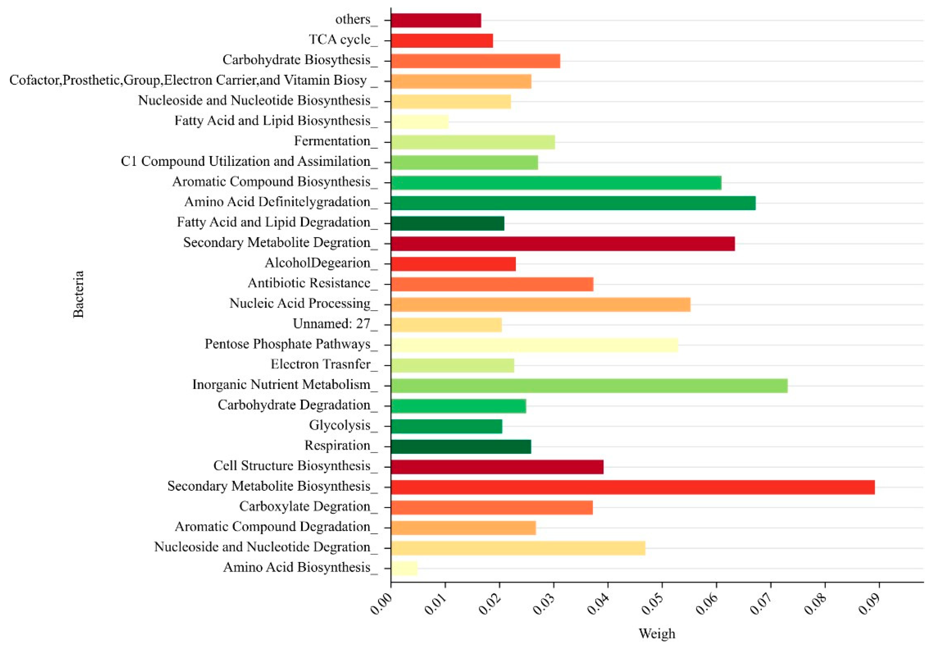
The 28 bacteria affecting the classification are brought into the random forest algorithm to calculate the feature importance magnitude, and the factors with the lowest importance degree are removed. Importance magnitude and the factors with the lowest degree are removed, and the process is repeatedly cycled until the factor feature importance degree are greater than the set threshold, that is, this stage is ended and the best feature subset was obtained. The importance magnitude of each bacterium is shown in the figure below (Figure 14).
The sensitivity of three algorithm model parameters is shown in Figure 15. As shown in the figure, the parameter sensitivity of random forest algorithm is most similar to the weight of each parameter calculated by entropy weight method. Therefore, the random forest algorithm is more optimal.
(3)
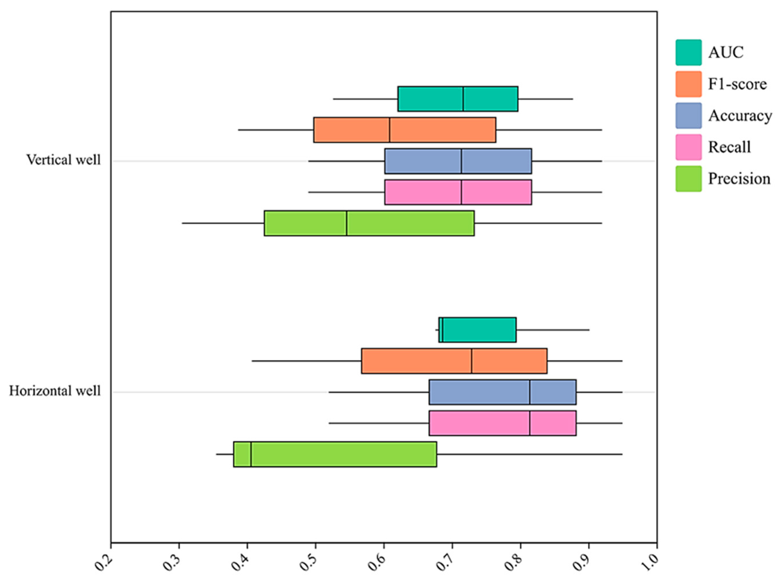
Randomly select 70% as the training set, and the remaining 30% as the test set. The maximum number of iterations is 150. Conduct sample prediction based on PSO random forest method. The confusion matrix is chosen as the evaluation metric for the improved algorithm. Based on the confusion matrix, four core metrics of the model can be derived: accuracy, accuracy, recall, and F1-score value. Accuracy is the ratio of the sum of true positive and true negative values to the total number of samples. The accuracy is also the ratio of the number of samples with the same prediction category and real category to the total number of samples. Accuracy is the sum of true positive values divided by true positive values and false positive values. Recall is the ratio of true positive values to the sum of true positive values and false negative values; F1-score combines two evaluation indexes, precision, and recall, and calculates the magnitude of each index when the true classification effect is the same for the predicted formation and the actual formation, i.e., the mean and weighted mean of each index, respectively. Set the parameters as shown in the following table. When the number of iterations reaches 150, the algorithm stops. The boundary and external conditions of PSO algorithm is shown in Table 3.
The classification effect of the traditional random forest classification model before the improvement is tested according to the above evaluation indexes and the testing process. The total number of samples tested for the improved PSO algorithm-based random forest classifier is 182 samples, and the final classification results of the algorithm are obtained as shown in the following table (Table 4).
From the above table, it can be seen that all the indicators in the improved algorithm are significantly better than the original random forest algorithm. Through the analysis of the above evaluation indexes, it can be seen that the prediction performance of the improved classification algorithm in this paper is much higher than that of the traditional classifier, and the prediction of the source formation of the liquid-producing formations has a more perfect effect, which is a good solution to the problem that the traditional classification effect is not satisfactory due to the high dimensionality of the data set and many noisy points and cannot be eliminated. The improved algorithm can effectively avoid the shortcomings of the traditional algorithm in updating the weights, the defects that the noise points are infinitely enlarged and the accuracy of the model is reduced. From the training data, the error rate is 0.03. At the same time, considering the influence of contaminated DNA sequence on accuracy in the whole process from sampling to laboratory treatment, this sequence should be identified as an unknown source category in the traceability process model. In conclusion, there is some uncertainty in this model.

3.3. Construction of Fluid-Producing Profiles

The random forest method is used to cluster the stratigraphic baseline and predict the categories of 5-month production fluid to realize the traceability of production fluid. So as to calculate the contribution rate of each formation and construct the production profiling map to realize the monitoring technology of production profiling at different stages. The five-month fluid production profile obtained by the random forest clustering and prediction method is shown below, where the vertical coordinates indicate each formation and the horizontal coordinates indicate the contribution rate of each formation to the production. The target layer is Formation 5 indicated in yellow (Figure 16). By constructing the production profiling of over 5 months, we have confirmed that this method can effectively monitor reservoir production performance for a long time.

4. Discussion

4.1. Advantages Compared with Traditional Production Profiling Technology

One of the major advantages of the production profiling technology proposed in this paper is that we first combine the DNA sequencing diagnostics technology with machine learning interpretation technology. The production profiling technology based on the microbial DNA sequencing diagnostics only needs to sample the cuttings and produced fluids, which does not pollute the formation and has no impact on operation. The second advantage of this technology is that we establish a production profiling interpretation model suitable for DNA sequencing results. This model can accurately and quickly trace the formation source of produced bacteria, and achieve the effect of showing the contribution rate of each formation. The PSO-optimized random forest clustering algorithm was constructed to describe the contribution of each formation to the production fluid. The precision reached 0.97, which improved by 0.02 compared to that before optimization. More specifically, the last advantage is that through sampling and sequencing of produced fluids at different periods, the production profiling in the whole stage can be obtained by the above machine learning model, so as to realize the long-term effective monitoring of unconventional reservoirs.

4.2. Future Research

The production profiling interpretation technology based on microbial DNA sequencing diagnostics constructed can monitor the reservoir. Meanwhile, the method can also be used for downstream applications. More specifically, the fracture height can be observed from the production profiling from different periods. The formations whose contribution rate exceed the average are the formations which the fracture passes. At the same time, it can be judged whether the fracture passes through the interlayer according to the produced fluids. After that, we l apply it to more reservoirs and compare it with the production data to verify its accuracy and make improvements. In the future, we will also focus on the sampling and sequencing of horizontal microbial samples and construct a 3D production profiling model, which will be of great help to horizontal well water exploration.

5. Conclusions

In this paper, we propose a production profiling interpretation technology based on microbial DNA sequencing diagnostics. Based on the microbial DNA sequencing results of the sampled cuttings and produced fluids up to 5 months, a high precision and speed fluid production profile traceability model based on PSO-optimized random forest clustering algorithm is constructed. It is used for the purpose of dynamic monitoring of reservoir production and long-time continuous monitoring. Specifically, the main conclusions are as follows:
(1)
A complete production profiling process including petroleum microorganism sampling and transportation methods, DNA extraction and PCR amplification methods, and DNA sequencing methods is established. The strategic baseline map is obtained by these methods, which reflects the bacteria species and their abundance in each formation. It illustrates the characteristics of formation bacteria and lays a foundation for the construction of the production profiling.
(2)
The random forest algorithm for the production profiling traceability algorithm is preferred by comparing the accuracy, precision, recall, F1-score, and running time of the three clustering methods of Naive Bayes, back propagation, and random forest. The PSO-optimized random forest clustering algorithm is constructed to describe the contribution of each formation to the production fluid. The precision reached 0.97, which improved 0.02 compared with that before optimization.
(3)
Previous studies about the present production profiling technologies have a short validity period, which can only reflect the temporary situation. Our laboratory results suggest that it is possible to conduct production profiling interpretation technology based on microbial DNA sequencing diagnostics of unconventional reservoirs in a simple and pollution-free way. By constructing the production profiling of over 5 months, we have confirmed that this method can effectively monitor reservoir production performance for a long time.

Author Contributions

Conceptualization, H.Y. and L.W.; methodology, H.Y.; software, H.Y.; validation, H.Y., X.Q. and Z.R.; formal analysis, H.Y.; investigation, H.Y., H.W.; resources, H.Y., Y.W.; data curation, H.Y.; writing—original draft preparation, H.Y.; writing—review and editing, H.Y.; visualization, H.Y.; supervision, S.W.; project administration, S.W.; funding acquisition, S.W. All authors have read and agreed to the published version of the manuscript.

Funding

This research received no external funding.

Data Availability Statement

The data presented in this study are available on request from the corresponding author.

Conflicts of Interest

The authors declare no conflict of interest.

Appendix A

(1)
Data standardization: In order to avoid the influence of the scale on the variable data, the data should be standardized first.
The normalization process used in this paper is Range0tol (graded regular transformation/specified transformation), and the transformed data has a minimum of 0 and a maximum of 1. The rest is in the interval [0, 1] with a graded difference of 1 and no dimension. The formula for calculating data normalization is shown below.
{ x i j * = x i f min x i j ( 1 i n ) R j x i j * = 0.5   When   R j = 0 When   R j 0 ( i = 1 , 2 n ; j = 1 , 2 . m )
(2)
Correlation analysis.
Correlation is a measure of the relevance of data attributes, and the correlation coefficient can be used to measure the degree of correlation between two things. In this paper, Pearson coefficient is used to determine the degree of correlation between different formations of bacteria.
ρ j = i = 1 17 ( x j i x ¯ j ) ( a i a ¯ ) i = 1 17 ( x j i x ¯ j ) 2 i = 1 17 ( a i a ¯ ) 2
where ρj is Pearson coefficient of the j-th formation, and j is one of the formations; i represents the abundance of 28 formations; a is the actual result.
(3)
Naive Bayes: each data sample of this classifier is represented by an n-dimensional feature vector [25,26]
X = {x1, x2, …, xn}, describing respectively for n feature formation attributes A1, A2, …, An of the samples with n metrics. The class labeling attribute C = {c1, c2, …, cm}. Given a sample of data X with unknown class label, the classification method will predict that X belongs to the class with maximum posterior probability (under condition X), i.e., the Naive Bayes classification assigns unknown samples to class c values independent of the classification attributes of the sample. When and only when P(ci|X) > P(cj|X), i ≠ j. So, the classification problem is transformed into finding the maximum P(Ci|X).
From Bayes’ theorem, we have
P ( c i X ) = P ( X c i ) P ( c i ) P ( X )
Maximize P(X|ci) P(ci). Assume that each category is conditionally independent, that is, there is no dependency between attributes. Therefore:
P ( X c I ) = k = 1 n p ( x k c I )
Here, P(ci), p(xk|ci), k = 1, 2, …, n can be calculated by maximum likelihood estimation
P ( c I ) = | T ( c i ) | | T | , p ( x k c I ) = T ( x k , c i ) | T ( c i )
Classify the unknown sample X, and calculate P(ci|X) P(ci) for each ci. Sample X is classified into class ci, if and only if P(X|ci) P(ci) > P(X|cj) P(cj), 1 ≤ j ≤ m, j ≠ i.
(4)
The algorithm steps of the random forest are as follows [27,28].
(A)
Draw the training set from the original sample set. In each round, n training samples are drawn from the original sample set using the Bootstrapping method (with put-back sampling). A total of k rounds are performed to obtain k mutually independent training sets.
(B)
One model is obtained using one training set at a time, and a total of k models are obtained for k training sets.
(C)
For the classification problem: the k models obtained in the previous step are used to obtain the classification results by voting; for the regression problem, the mean value of the above models is calculated as the final result.
(5)
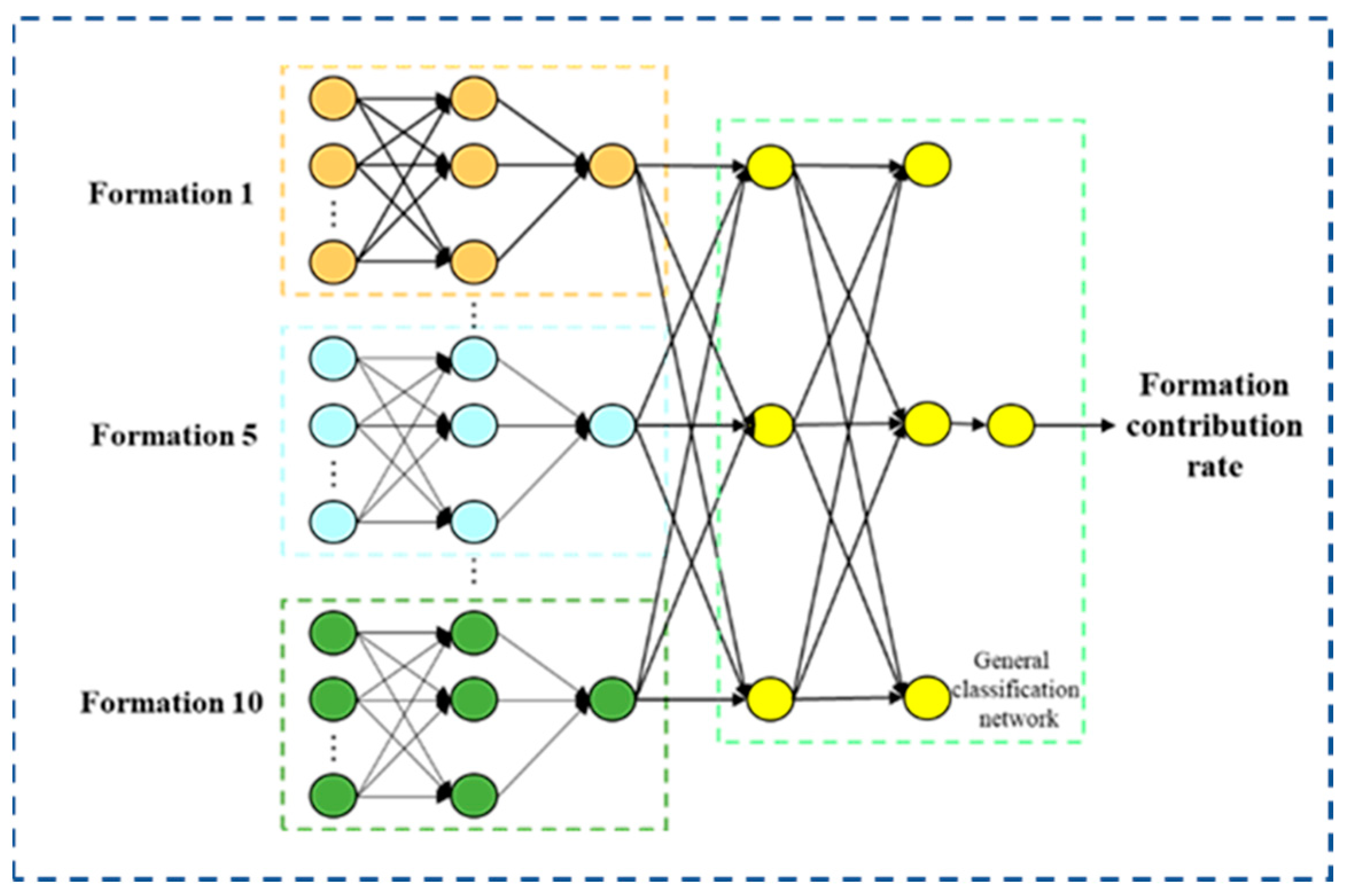
Back propagation: where the input layer of this model is the sequencing data of the stratigraphic baseline, the implicit layer is the new clustering result, and the output layer is the probability that the fluid production originates from each formation, the contribution rate of each formation. The output of the implicit layer is set to Fj, the output of the output layer is set to Ok, the excitation function of the system is set to G, and the learning rate is set to β. Then the mathematical relationship between its three layers is as follows [29].
The desired output of the system is set to Tk, then the error E of the system can be expressed by the variance of the actual output value and the desired target value with the following relational expression.
{ F j = G ( i = 1 m ω i j x i + a j ) O k = j = 1 l F j ω j k + b k
Using the gradient descent principle, the updating formula of system weight and offset is as follows
{ ω i j = ω i j + β F j ( 1 F j ) x i k = 1 n ω j k e k ω j k = ω j k + β F j e k { a j = a j + β F j ( 1 F j ) x i k = 1 n ω j k e k b k = b k + β e k
E = 1 2 k = 1 n ( T k O k ) 2
e k = T k O k
(6)
Accuracy is the percentage of all samples with correct predictions divided by the total sample, and generally speaking the closer to 1 the better. Its meaning is the proportion of predicted and actual categories that are both 1 to the predicted category of 1. For this data set is the total number of samples with the same actual source of fluid production for that formation and the predicted source of fluid production for that formation as a percentage of the predicted source of fluid production for that formation. The formula for this is.
P r e c i s i o n = T P T P + F P
A c c u r a c y = T P + T N T P + T N + F P + F N
(7)
Precision, which indicates the proportion of the number of samples that are actually 1 among the number of samples with a prediction result of 1.
(8)
Recall, which indicates the proportion of all samples with true 1 that are correctly predicted by us. A higher recall means that we try to capture as many minority classes as possible, and a lower recall means that we do not capture enough minority classes. For this dataset the meaning is expressed as the proportion of the total number of samples with the same actual source of fluid production as the predicted source of fluid production in the formation to the actual source of the formation. The formula for this is:
R e c a l l = T P T P + F N
(9)
In order to balance both precision and recall, we create a summed average of the two numbers as a comprehensive metric to consider the balance between them, called F measure. The F measure is distributed between [0, 1], and the closer to 1, the better. The significance for this dataset is that for a high proportion of the total number of samples where both the actual and predicted sources of fluid production are from that formation to the predicted source of that formation, it will inevitably lead to a decrease in the proportion of the total number of samples where both the actual and predicted formations are from that formation to the actual source of that formation. The ideal F1-score metric is one in which the difference between the accuracy and recall rates is small and both are improved, and the formula is:
F m e a s u r e = 2 1 P r e c i s i o n + 1 R e c a l l = 2 × P r e c i s i o n × R e c a l l P r e c i s i o n + R e c a l l
(10)
The ROC curve, known as receiver operating characteristic curve, reflects the trend of true positive rate (TPR) with false positive rate (FPR), and is a curve plotted with true positive rate (sensitivity) as the vertical coordinate and false positive rate (1-specificity) as the horizontal coordinate. According to the position of the curve, the whole graph is divided into two parts. The area of the lower part of the curve is called AUC (area under curve), which is used to indicate the prediction accuracy, and the higher the AUC value, i.e., the larger the area under the curve, the higher the prediction accuracy. The higher the AUC value, the larger the area under the curve, the higher the prediction accuracy. The closer the curve is to the upper left corner (the smaller the X and the larger the Y), the higher the prediction accuracy.

References

  1. Lv, Y.; Wang, B.; Huang, W.; Han, E. Integrated technology of horizontal well water detection and testing. Pet. Field Mach. 2011, 40, 93–95. [Google Scholar]
  2. Di, D.; Guo, X.; He, Z.; Pang, W. Testing Technology of Intelligent Tracer Production Profile. Oil Gas Well Test. 2021, 30, 44–49. [Google Scholar]
  3. Chang, Q.; Liu, Y.; Lu, W.; Wang, X.; Zhang, H.; Zhang, L. Diagnostic technology of trace substance tracers for shale oil horizontal well pressure drainage. Oil Gas Well Test. 2021, 30, 32–38. [Google Scholar]
  4. Yue, P. Research on logging technology of liquid production profile. Petrochem. Technol. 2016, 23, 147. [Google Scholar]
  5. Du, S.; Liu, Q.; Luo, W.; Ma, G. Evaluation and application of liquid production production profiling technology in low permeability reservoirs. Petrochem. Appl. 2018, 37, 87–90. [Google Scholar]
  6. Cui, H. Research on Comprehensive Interpretation Method of Annular Fluid Production Profile. J. Pet. Nat. Gas 2008, 3, 266–268. [Google Scholar]
  7. Qin, D.; Gao, Y.; Yu, Y. Evaluation on the adaptability of liquid production production profiling of preset downhole traction horizontal wells. Petrochem. Technol. 2016, 23, 278. [Google Scholar]
  8. Chen, E.Y.; Chen, R.B. Monitoring Microbial Corrosion in Large Oilfield Water Systems. J. Pet. Technol. 1984, 36, 1171–1176. [Google Scholar] [CrossRef]
  9. Tang, Y.; Xu, K.; Gu, L.; Yang, F.; Gao, J.; Ren, C.; Wang, G. Research Progress in Theory and Technology of Microbial Exploration for Oil and Gas. Pet. Exp. Geol. 2021, 43, 325–334. [Google Scholar]
  10. Brown, L.R. Microbial enhanced oil recovery (MEOR). Curr. Opin. Microbiol. 2010, 13, 316–320. [Google Scholar] [CrossRef] [PubMed]
  11. Sawadogo, J.; Haggertty, M.; Mallory, C.; Huchton, J.; DeAngelis, W.; Price, C. Impact of Completion Design and Interwell Communication on Well Performance in Full Section Development: A STACK Case Study Using DNA Diagnostics. In Proceedings of the SPE Annual Technical Conference & Exhibition, Houston, TX, USA, 12–14 October 2020. SPE-201726-MS. [Google Scholar]
  12. Ursell, L.; Hale, M.; Menendez, E.; Zimmerman, J.; Dombroski, B.; Hoover, K.; Ishoey, T. High Resolution Fluid Tracking from Verticals and Laterals Using Subsurface DNA Diagnostics in the Permian Basin. In Proceedings of the SPE/AAPG/SEG Unconventional Resources Technology Conference, Denver, CO, USA, 22–24 July 2019. [Google Scholar]
  13. Sawadogo, J.; Ursell, L.; Reeve, N.; Schlecht, M. Mature Fields—Optimizing Waterflood Management Through DNA Based Diagnostics. In Proceedings of the Abu Dhabi International Petroleum Exhibition & Conference, Abu Dhabi, United Arab Emirates, 9–12 November 2020. [Google Scholar]
  14. Percak-Dennett, E.; Liu, J.; Shojaei, H.; Luke, U.; Thomas, I. High Resolution Dynamic Drainage Height Estimations using Subsurface DNA Diagnostics. In Proceedings of the SPE Western Regional Meeting, San Jose, CA, USA, 24 April 2019. [Google Scholar]
  15. Silva, J.; Ursell, L.; Percak-Dennett, E. Applying Subsurface DNA Diagnostics and Data Science in the Delaware Basin. In Proceedings of the SPE Hydraulic Fracturing Technology Conference and Exhibition, The Woodlands, TX, USA, 23 January 2018. [Google Scholar]
  16. Zhang, Y.; Dekas, A.E.; Hawkins, A.J.; Parada, A.E.; Gorbatenko, O.; Li, K.; Horne, R.N. Microbial Community Composition in Deep-Subsurface Reservoir Fluids Reveals Natural Interwell Connectivity. Water Resour. Res. 2020, 56, e2019WR025916. [Google Scholar] [CrossRef] [Green Version]
  17. Zhang, Y.; Horne, R.N.; Hawkins, A.J.; Primo, J.C.; Gorbatenko, O.; Dekas, A.E. Geological activity shapes the microbiome in deep-subsurface aquifers by advection. Proc. Natl. Acad. Sci. USA 2022, 119, e2113985119. [Google Scholar] [CrossRef] [PubMed]
  18. Knights, D.; Kuczynski, J.; Charlson, E.; Zaneveld, J.; Mozer, M.C.; Collman, R.G.; Bushman, F.; Knight, R.; Kelley, S.T. Bayesian community-wide culture-independent microbial source tracking. Nat Methods 2011, 8, 761–763. [Google Scholar] [CrossRef] [PubMed] [Green Version]
  19. Shenhav, L.; Thompson, M.; Joseph, T.A.; Briscoe, L.; Furman, O.; Bogumil, D.; Mizrahi, I.; Pe’er, I.; Halperin, E. FEAST: Fast expectation-maximization for microbial source tracking. Nat Methods 2019, 16, 627–632. [Google Scholar] [CrossRef] [PubMed]
  20. Alberti, L.; Angelotti, A.; Antelmi, M.; La Licata, I. Borehole Heat Exchanger simulations in aquifer: The borehole grout influence in Thermal Response Test modeling. In Proceedings of the 87° Congresso della Società Geologica Italiana, Milan, Italy, 10–12 September 2014. [Google Scholar]
  21. Bao, Y.J.; Xu, Z.; Li, Y.; Yao, Z.; Sun, J.; Song, H. High-throughput metagenomic analysis of petroleum-contaminated soil microbiome reveals the versatility in xenobiotic aromatics metabolism. J. Environ. Sci. 2017, 56, 25–35. [Google Scholar] [CrossRef] [PubMed]
  22. Dai, X.; Wang, Y.; Luo, L.; Pfiffner, S.M.; Li, G.; Dong, Z.; Xu, Z.; Dong, H.; Huang, L. Detection of the deep biosphere in metamorphic rocks from the Chinese continental scientific drilling. Geobiology 2021, 19, 278–291. [Google Scholar] [CrossRef] [PubMed]
  23. Lasken, R.; McLean, J. Recent advances in genomic DNA sequencing of microbial species from single cells. Nat. Rev. Genet. 2014, 15, 577–584. [Google Scholar] [CrossRef] [PubMed]
  24. Hu, M.; Zhang, S. A leaf node weighted Random Forest algorithm based on PSO optimization. Mod. Comput. 2022, 28, 1–4. [Google Scholar]
  25. Xie, B. Application of Naive Bayesian Classification in Data Mining. J. Gansu Union Univ. Nat. Sci. Ed. 2007, 21, 79–82+91. [Google Scholar]
  26. Liu, W.; Liang, S.; Wang, C. Naive Bayesian classification method based on weighted kernel principal component. J. Chang. Univ. Technol. China 2022, 43, 610–618. [Google Scholar]
  27. Adeeyo, Y. Random Forest Ensemble Model for Reservoir Fluid Property Prediction. In Proceedings of the SPE Nigeria Annual International Conference and Exhibition, Lagos, Nigeria, 1–3 August 2022. [Google Scholar]
  28. Gamal, H.; Alsaihati, A.; Elkatatny, S.; Abdulraheem, A. Sonic Logs Prediction in Real Time by Using Random Forest Technique. In Proceedings of the ARMA/DGS/SEG 2nd International Geomechanics Symposium, Virtual, 1–4 November 2021. [Google Scholar]
  29. Zhao, H.; Geng, Y.; Liu, Z.; Wang, W.; Zhou, Z.; Kao, J. Study on Fracture-Cavity Instability of Carbonate Rocks Based on Back-Propagation (BP) Back propagation. In Proceedings of the 53rd U.S. Rock Mechanics/Geomechanics Symposium, New York, NY, USA, 23–26 June 2019. [Google Scholar]
Figure 1. Significance of DNA sequencing of petroleum-based microorganisms.
Energies 16 00358 g001
Figure 2. Produced fluids profile model based on microbial DNA sequencing.
Energies 16 00358 g002
Figure 3. Heat map of the accuracy of sequencing results. The higher the biomass and the higher the number of samples, the greater the accuracy of sequencing results. Due to the low microbial biomass of cuttings, the accuracy of sequencing results is greatly affected. Therefore, a strict quality control process is required to ensure the accuracy of downstream analysis.
Energies 16 00358 g003
Figure 4. Quality control of DNA markers. The valid area meets both the medium biomass and downstream analysis mass fraction above 0.8, so it can be used for downstream analysis. The sequencing data in the biomass greater than 30 region is considered to be caused by microbial overgrowth, and insufficient biomass will seriously affect accuracy. So, the overbreeding area and invalid area also cannot be used for downstream analysis.
Energies 16 00358 g004
Figure 5. Data on the input side of the produced fluids traceability model. The data includes bacteria species and their percentage in each formation.
Energies 16 00358 g005
Figure 6. Sample data interpretation and clustering model. The establishment of the formation traceability model of the production fluid first requires converting the DNA sequencing results of the samples into a matrix, where each column represents a layer and each row represents a formation feature. A new layer is obtained by clustering the sample data by three methods: random forest, back propagation, and Naive Bayes. After that, the formations contained in the yield sequencing results are clustered as features to sub-trace the probability of originating from each formation.
Energies 16 00358 g006
Figure 7. Formation correlation heat map. It can be understood that the correlation coefficient of Cofactor, Prosthetic, Group, Electron Carrier, and Vitamin Biosy and Aromatic Compound Degradation is 0.71, Cell Structure Biosynthesis and C1 Compound Utilization and Assimilation had a correlation coefficient of 0.674.
Energies 16 00358 g007
Figure 8. (a) Network diagram of Naïve Bayes. (b) Network diagram Naïve Bayes, back propagation.
Energies 16 00358 g008
Figure 9. Network diagram of random forest classifier. The back propagation includes an input layer, a hidden layer, and an output layer.
Energies 16 00358 g009
Figure 10. Stratigraphic baseline map. The stratigraphic baseline map shows the formations contained at different depths and their abundance, and different formations are indicated by different colors.
Energies 16 00358 g010
Figure 11. Comparison of ROC of three methods. The area under the curve is called AUC (area under curve), which is used to indicate the prediction accuracy. The accuracy of random forest is greater than back propagation is greater than Naïve Bayes.
Energies 16 00358 g011
Figure 12. Overall performance of the random forest algorithm in vertical and horizontal wells. No matter vertical well or horizontal well, the accuracy of the optimized random forest algorithm is very high. At the same time, it also proves that the random forest algorithm is applicable to the production profiling of vertical wells and horizontal wells.
Energies 16 00358 g012
Figure 13. Comparison of the running time of the three algorithms. Whether vertical or horizontal wells, the running time of random forest is shorter than that of back propagation, and the naive Bayesian algorithm takes the longest running time.
Energies 16 00358 g013
Figure 14. Histogram of importance of each bacterium. Secondary Metabolite Biosynthesis has the highest weight; Amino Acid Biosynthesis has the lowest weight.
Energies 16 00358 g014
Figure 15. The sensitivity of three algorithm model parameters. The random forest model is shown in the green bar, the back propagation model is shown in the orange bar, the Naïve Bayes model is shown in the blue bar.
Energies 16 00358 g015
Figure 16. Five months production profiling. The fracturing operation started on day 15, and the contribution rate of the target formation increased significantly from day 15, which matches the actual production data. The dashed line in the graph shows the average contribution rate of all formations. It is obvious from the graph that the contribution rate of Formation 2, 3, 4, 5 and 6 exceeds the average, which leads to the conclusion that the fracture height extends up to Formation 2 and down to Formation 6.
Energies 16 00358 g016
Table 1. Comparison of accuracy of three methods with horizontal well data.
Vertical WellAUCF1-ScoreAccuracyRecallPrecision
Random Forest0.87750.920.920.920.92
Back Propagation0.71650.6090.7140.7140.546
Naïve Bayes0.52610.3870.490.490.305
Table 2. Comparison of accuracy of three methods with direct well data.
Horizontal WellAUCF1-ScoreAccuracyRecallPrecision
Random Forest0.90160.950.950.950.95
Back Propagation0.68650.7290.8140.8140.406
Naïve Bayes0.67610.4070.520.520.355
Table 3. The boundary and external conditions of PSO algorithm.
ParameterValue
Maximum Iterations150
Inertia weight0.9
Individual learning factors2
Sociology Department Factor2
Maximum iteration speed4
Table 4. Comparison of accuracy before and after algorithm improvement under horizontal well data.
Horizontal WellAUCF1-ScoreAccuracyRecallPrecision
Random Forest0.90160.950.950.950.95
Random Forest Based
on PSO Optimization
0.93420.970.970.970.97
Disclaimer/Publisher’s Note: The statements, opinions and data contained in all publications are solely those of the individual author(s) and contributor(s) and not of MDPI and/or the editor(s). MDPI and/or the editor(s) disclaim responsibility for any injury to people or property resulting from any ideas, methods, instructions or products referred to in the content.

