Abstract
Electric power systems have experienced the rapid insertion of distributed renewable generating sources and, as a result, are facing planning and operational challenges as new grid connections are made. The complexity of this management and the degree of uncertainty increase significantly and need to be better estimated. Considering the high volatility of photovoltaic generation and its impacts on agents in the electricity sector, this work proposes a multivariate strategy based on design of experiments (DOE), principal component analysis (PCA), artificial neural networks (ANN) that combines the resulting outputs using Mixture DOE (MDOE) for photovoltaic generation prediction a day ahead. The approach separates the data into seasons of the year and considers multiple climatic variables for each period. Here, the dimensionality reduction of climate variables is performed through PCA. Through DOE, the possibilities of combining prediction parameters, such as those of ANN, were reduced, without compromising the statistical reliability of the results. Thus, 17 generation plants distributed in the Brazilian territory were tested. The one-day-ahead PV generation forecast has been considered for each generation plant in each season of the year, reaching mean percentage errors of 10.45% for summer, 9.29% for autumn, 9.11% for winter and 6.75% for spring. The versatility of the proposed approach allows the choice of parameters in a systematic way and reduces the computational cost, since there is a reduction in dimensionality and in the number of experimental simulations.
1. Introduction
The increase in the share of renewable energies in the electricity matrix around the world is a demand of economic, social and environmental interest [1]. The broad perspectives for the use of fossil fuels reinforce the potential of these resources to supply electricity [2]. Authors in [3] cite solar energy as the main focus for investors in recent years. In this context, to deal with unexpected changes in weather conditions and to carry out a rigorous control and management of solar energy in smart systems, it is necessary to adopt photovoltaic (PV) energy generation prediction models. The effectiveness of these models impacts system efficiency and safety, and the measurements provide reliable information for energy customers and suppliers [4].
However, several authors point out that the meteorological factors and the distribution networks’ infrastructure conditions are aspects that strongly influence the efficient use of solar energy as an alternative source [5]. The influence of some meteorological factors was tested in several studies, which reinforced the urgent need to propose methods for monitoring phenomena and robust forecasting models [6]. There are several methodologies for predicting solar irradiance, the most common being analytical, stochastic, empirical, statistical models and artificial neural networks [6].
Artificial neural networks have been widely used to predict photovoltaic power generation [7]. Some research has pointed out the advantages of big data analysis for renewable energy forecasting [8].Works [9,10,11] present predictive solutions based on supervised or unsupervised machine learning. For this sake, such as the integrated autoregressive moving average model, pattern sequence prediction and artificial neural network (ANN) models are discussed.
The PV output power prediction model developed by [7] was applied for short-term prediction, specifically, one hour ahead. In this case, the authors used the extreme learning machine (ELM) algorithm. For day-ahead photovoltaic output power prediction, the researchers tested the model using daily average solar radiation (W/m²), wind speed (m/s), ambient and module temperature (°C). The ELM-based model was compared with two other models, one using support vector regression (SVR) and the other using ANN. The results showed that the ELM presented greater precision and less computational time in the short-term prediction of daily and hourly photovoltaic output power.
To improve the ELM, [12] implemented a new model called expanded ELM (EELM) for photovoltaic energy forecasting. EELM breaks new ground by allowing automatic selection of hidden layer number and random input weights. However, the higher extrapolation capabilities of the EELM have only been demonstrated for a forecast horizon of less than 1 h. Based on the research works mentioned above, the effectiveness of a photovoltaic power generation prediction model can be made even more accurate through experimentation with viable scenarios. According to [13], machine learning methods are very effective for predicting photovoltaic energy generation, given the non-linear nature of the variables. However, the authors indicate that combined methods should be adopted in order to capture the stochastic characteristic of solar irradiance and the high variability of measurements. Therefore, the main objective of this work is to propose a multivariate strategy based on design of experiments (DOE), principal component analysis (PCA), artificial neural networks (ANN) that combines the resulting outputs using Mixture DOE (MDOE) for photovoltaic generation prediction a day ahead.
DOE is a statistical optimization tool in which each experimental run is a test and allows the investigator to discover some information about a process or system [14]. Subsequently, the best configurations observed in the DOE approach are maintained, through a cluster analysis, to form a combined forecast. An ensemble forecast tends to improve the results of individual [15] models. The proposed combination considers that a mixture analysis calculates the definition of the set weights. Finally, the combined result obtained is analyzed to determine if it has equivalence with the original dataset. This analysis is performed using the confidence ellipse for the data at a 95% confidence level.
2. Literature Review
The intermittent nature of solar generation brings operational challenges to the electrical system, which compromises the quality and security of supply, and can lead to voltage fluctuations and harmonic distortion [16]. One way to deal with this problem is to define accurate predictions [17].
The work developed by [18] proposed a method for predicting photovoltaic generation using a hybrid model that combines signal decomposition, artificial intelligence models, deep learning models and swarm optimization model. The performance of the proposed system is not discussed if the amount of data increases.
The model proposed by [19] investigates the performance of LSTM, convolutional, and hybrid convolutional–LSTM networks on residential photovoltaic generation data. The evaluation metrics were used to compare the results with a decomposable time series forecasting model known as Prophet, considering different time scales. The author considers forecasts individually and does not mention whether the combination of results improves the performance of forecast models.
The authors at [20] have pursued a multivariate approach, based on the convolutional neural network (CNN) that considers the use of climate variables in the forecasting process. The results, at the end of this computation, are combined to improve the final output. However, the elucidated model does not offer tools to the analyzer to indicate which variables/parameters may interfere with the forecast results.
In some cases, finding variables that can help the forecasting process can be a challenging task. From the work developed by [21], it is interesting to observe the use of satellite images to compose the input data of the forecast models. The proposal is based on convolutional long short term memory network (Conv–LSTM) and extreme gradient boosting (XGBoost). However, the authors do not explore the combined prediction and dimensionality reduction of the data (since satellite images require more computational space compared to textual data).
The combined forecast, based on scenarios, was explored in [22] and showed better results compared to the use of individual models. Even so, the work does not discuss how the parametric variation of the models influences the result, nor does it present a model for reducing the dimensionality of the data.
Clustering of climate data by season of the year was considered in [23] using the Fuzzy C-Means (FCM) algorithm for one-day-ahead forecasting. The model based on least squares support vector machine (LSSVM) outperformed other forecasting models. The work does not consider the combined forecast.
An approach based on gated recurrent unit (GRU), random forest was compared with the results of LSTM and RNN, using daily and monthly data [24]. The results achieved are interesting, but the work does not consider the seasonal separation of the data and does not allow the analyzer to verify which parameters influence the forecast result.
The research carried out in [25] proposes an approach for clustering regions and forecasting photovoltaic generation, which lists locations with better viability for the installation of photovoltaic panels. A probabilistic method combined with machine learning models for forecasting photovoltaic generation is considered to be more suitable for the study horizon and data discretization, which is monthly. A study was carried out in Mexico in regions with meteorological and topographic variability, finding that the points with the highest solar incidence are not always the points that promote the highest yield of energy generation.
Artificial neural networks using the Levenberg–Marquardt training algorithm were considered in the research conducted by the authors in [26]. The selected meteorological variables include temperature, relative humidity, solar irradiance and wind speed. Keeping the angle definitions, the study showed promise. However, the authors do not detail how the parametric variation of the forecast model impacts the results.
The very short-term forecast conducted by [27] analyzes the data forecast with discretization varying from minute to minute related to the cloud accumulation indicator. In this study, the authors highlighted the use of neural networks and random forest models. The data considered in this study are not subjected to dimensionality reduction and the parametric configuration of the models is not detailed.
A study conducted by [28] analyzed the performance of a regression network and particle swarm optimization model for a dataset from a plant located in Brazil. The time horizon considered was one day ahead with hourly discretization. The model parameters were statically defined and the impact of their variation on the prediction results was not considered.
The key contributions of this research, trying to fill these gaps, are summarized in:
- Reduce the dimensionality of climate data to facilitate the capture by machine learning models of the intrinsic non-linearity of these time series, and mitigate possible noise that may exist in the data.
- Group similar days using cluster analysis technique to compose the forecast. This also reduces the amount of data finished by the machine learning model.
- Parameterize the execution of the experiment using the DOE statistical tool, which reduces the search space, saving computational resources and time without losing statistical reliability.
The scientific community has turned its eyes to the various deep learning models [29] and their example-based training applications. Some variations of these algorithms can be mentioned, such as long short term memory networks (LSTMs), convolutional neural networks (CNNs), radial basis function networks (RBFNs), multilayer perceptrons (MLPs).
LSTMs are a specialization of recurrent neural network (RNN) that preserve information over a period of time, learning and storing that information whose interdependence is observed, being widely used in time series forecasting problems. The multiple layers of CNNs have filters that enable performing convolution operations and are especially useful for extracting features from data. RBFNs have the versatility to solve classification, regression and prediction problems because they are feedforward-type networks, which means input, hidden and output layers are present and the activation functions are a radial basis type. MLPs are also a type of feedforward network where input and output layers are fully connected, so weights and bias are calculated and activation functions are applied to compute the result. Table 1 shows a brief analysis of the application of these models recently.

Table 1.
Some recent applications of deep learning models.
3. Proposed Methodology
The proposed methodology is summarized in Figure 1, and essentially uses DOE, PCA and ANN. The methodological process of this work is based on research [37]. The authors encourage the application of this model due to its versatility, which reduces the computational effort and tends to produce good results. To facilitate the reader’s understanding, each topic that composes the steps of this process is detailed.
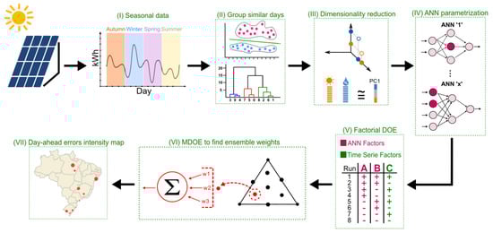
Figure 1.
Proposed strategy for photovoltaic (PV) generation forecast using cluster analysis, principal component analysis (PCA), artificial neural network (ANN), design of experiments (DOE) and Mixture DOE (MDE). Source: own authors.
The proposed methodology’s application helps operate active distribution networks and emerging transmission systems, since the operator is informed about the actual generation availability in the next time window. Thus, generation and system configuration adjustments are possible, enabling the utilities to provide a reliable service.
In addition to the use of DOE, this work introduces the use of principal component analysis to reduce the dimensionality of climate data, with minimal loss of information, for training the machine learning model.
3.1. Data Collection and Preparation
An essential step that precedes data analysis is collecting and preparing time series. This data is often difficult to obtain due to the data protection policy of local generation plants [38], which can compromise advances of photovoltaic generation forecasting. The entire forecasting process can be compromised if this step is not seriously considered [39]. This step covers correcting missing data, normalizing data, adjusting data resolution and grouping data [40]. Real photovoltaic generation data were used from the PVOutput.org [41] repository, with the daily resolution, except for the data from the generation plants of the cities of Machado and Passos, which were acquired from the Federal Institute of South of Minas Gerais IFSULDEMINAS.
Seventeen generating units are considered in this study; each one has a different generation capacity and is geographically separated throughout the Brazilian territory. The reason for choosing these units was due to the availability and quality of data in the time horizon of the study. Missing or null data were disregarded.
The climatic data were obtained through the National Institute of Meteorology (INMET) [42], considering the weather stations closest to the previously selected photovoltaic generation plants, covering sixteen parameters: instantaneous temperature (°C), maximum temperature (°C), minimum temperature (°C), instantaneous humidity (%), maximum humidity (%), minimum humidity (%), instantaneous precipitation (°C), maximum precipitation (°C), minimum precipitation (°C), pressure instantaneous (hPa), maximum pressure (hPa), minimum pressure (hPa), wind speed (m/s), wind direction (°), wind gust (m/s) and radiation (KJ/m²).
In order to facilitate the identification of each photovoltaic generation plant, and their respective climatic data, the closest city to that measurement point was considered and these characteristics are listed in the following Table 2:
Table 2.
Detailing of photovoltaic generation plants.
The data series was divided into seasons, since each one presents different characteristics that can be relevant factor for the success of a more accurate forecast. The increase or decrease in the efficiency of the panels can be influenced by environmental factors in the region, such as wind speed, humidity, dust, temperature, among others [43], justifying the segmentation by season. In Brazil, summers are hot and humid, with a predominance of rain in several regions, while winter causes drought and cold. From Figure 2, it is possible to identify these periods throughout the months of the year.

Figure 2.
Four subdivisions of the periods of the year for the Brazilian territory. Hot and rainy summers, dry winters and windy autumns. Source: own authors.
Therefore, when it comes to photovoltaic generation, the panels can gain or lose efficiency due to numerous uncontrollable factors, related to the season [44], such as the accumulation of dust, predominance of clouds over the generation area, cooling of solar cells, etc. The separation of data into seasons aims to mitigate these effects so that the forecast model does not suffer from the inconsistencies that can be generated in the training process.
Since each photovoltaic generation plant has different generation capacity, and the climatic data have different measurement units, two ways of normalizing the data were considered, placing them in a feasible scale for the optimization process through algorithms of machine learning.
The first, which uses the maximum and minimum values of time series, rescales the data within the interval between 0 and 1 and is observed in Equation (1), where “” is the observed value, “” the minimum value of time series and “” the highest value [45]:
The other normalization technique, known as standardization or Z-Score method, uses the mean and standard deviation of the series itself, making the normalized value centered around the mean with unit standard deviation [46]. The standardization calculation is performed according to the Equation (2), where “” is the observed value, “” is the mean and “” the standard deviation.
3.2. Hierarchical Cluster–Grouping of Similar Days
After dividing the data series into seasons, the hierarchical clustering technique was used to group the days with certain similarity levels. These grouping methods initially consider each data point (or object) as a group [47]. Then, similar objects begin to coalesce to form groups. Figure 3, in a simplified way, schematizes the separation of the six data points into groups and structures the minimalist representation of the respective dendrogram. The distance between the groups that form is calculated by the linkage method, which in this work considered the following two: Complete and Ward.
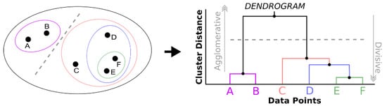
Figure 3.
Schematic example of grouping six data points and their representation in the dendrogram. Source: own authors.
The Complete linkage method, also known as the furthest neighbor, calculates the maximum distance between an object in a given cluster and another object belonging to another cluster. In general, the diameter of the formed groups tends to have similar sizes. The Complete method was chosen because it performs well in certain cases [48] and is represented by Equation (3), where “” is the distance between the clusters “” and “” and “” symbolizes an object “” in the cluster “” [49].
Ward’s linkage method minimizes the sum of squares within each cluster, and the distance between these clusters is calculated by the sum of squared deviations from the points to the centroids. In this case, each group tends to have the same number of objects. The choice of Ward’s method to compose the experiments of this work was because that it demonstrates good separability between groups and consistency [50]. Equation (4) calculates the Ward’s distance, where “” represents the number of objects present in cluster “y”, and so on.
3.3. Principal Component Analysis (PCA) for Dimensionality Reduction
PCA is a multivariate tool widely used in the literature [51]. It reduces the dimensionality of the dataset, to an uncorrelated set, known as principal components, that may explain the whole original set. It can separate out information that is redundant and random. The representation of the variance of the data tends to be in the first components (where the first component has the maximum explanation compared to the other components [52] and so on). The noise tends to be in the last components, that is, the principal components are uncorrelated linear combinations [53] of the original variables weighted by the eigenvalues.
According to [54], it can be described briefly by considering observation vectors and the respective mean vector (where the ellipsoid axis origin will be). The change to the origin is described . Rotating the axis centered on the mean results in principal components, which are uncorrelated. The rotation movement multiplies each by an orthogonal matrix , according to Equation (5):
If is orthogonal, then , and the distance to the origin remains the same, as observed in Equation (6):
The rotation transforms to a point, keeping the same distance from the origin. The calculation of matrix allows the discovery of the axes of the ellipsoid, making uncorrelated. In this way, the sample covariance matrix of , is desired to be diagonal, as in Equation (7):
where is the covariance matrix of . Since are the eigenvalues of and an orthogonal matrix in which the columns are the normalized eigenvectors of , . The transpose of matrix is the orthogonal matrix that diagonalizes , as shown in Equation (8):
so that is the normalized th eigenvector of . The principal components are represented by the variables , , …, in . The diagonal elements of are eigenvalues of . This makes the eigenvalues of the variances of the principal components , as described in Equation (9):
Since the eigenvalues are the variances of the principal components, the expression of percentage of explanation by the first components is used:
Reducing the dimensionality of meteorological data, for training machine learning models, avoids overfitting and allows the original data to be replaced by this new dataset, reduced, but retains most of the original information [55].
The application of the PCA method extends to problems in different areas and has contributed to interesting solutions. For example, recently, some authors [56] have proposed a variation of the PCA combined with the modified affinity propagation clustering algorithm (called PCA-MAP) to classify tourist preference information. It is also worth mentioning the work by [57] that explores day-ahead carbon price prediction using PCA combined with several machine-learning methods, providing dimensionality reduction from 37 variables to only 4.
This work considers data dimensionality reduction in two specific cases, depending on the methodological process, defined by the consideration, or not, of the meteorological variables.
Figure 4 exemplifies the structure of the data collected, with each line representing a measurement day and each column representing an observed variable. The first column consists of the photovoltaic generation data. The others (2 to 17) comprise the climatic variables. The PCA is applied, when the climatic variables are considered in the experimental run, in columns 2 to 17 of Figure 4.

Figure 4.
PCA is applied to reduce the climatic variables of columns 2 to 17. Source: own authors.
On the other hand, when the experimental process does not consider the climatic variables, but only the photovoltaic generation variables, a data restructuring is necessary. In this case, the data stacking process for model training is exemplified in Figure 5. Here, six generation days before the observed measurement day are chosen. These six days will compose the training data referring to that observed day, as observed in Figure 5 “A” (green) and “B” (yellow) markings. As one walks through the generation data structure, the sliding window forms new training data for the measurements of subsequent days. Finally, the PCA is applied to this dataset (columns 2 to 7). The region highlighted in red is disregarded in this situation because it has many null cells, which represents noise for the prediction model.
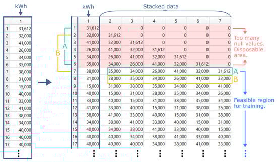
Figure 5.
Reorganizing generation data for training: stacking data for training based on information from the previous 6 days. Source: own authors.
Thus, when the climatic variables are considered, there is a reduction of 16 observations. When only the photovoltaic generation is considered, there is a formation of six variables for dimensionality reduction.
3.4. Artificial Neural Networks (ANN) Parametrization
There are numerous situations in which using of artificial neural networks is satisfactory [58], such as pattern recognition, classification, fault detection and PV generation forecasting [59]. Since the photovoltaic generation prediction problem has, in essence, non-linear characteristics, machine learning models try to efficiently capture these variations and present them in the output [60], but with the premise that there is no model in the literature that performs well in all cases. ANNs were chosen in this work because of their superior performance compared to other machine learning models [61].
Essentially, an ANN is made up of three layers [62], in its minimal architecture. The first layer is known as data input. This layer may contain one or more neurons. The second layer, known as the intermediate (or hidden) layer, may not be unique and has several neurons set by the analyzer, independent of the number chosen for the first layer. Finally, there is the last layer, or output layer, where the results are obtained after the training and testing process.
Neurons are present in all layers and constitute the network’s architecture, and can be added (or removed) from each layer as it fits well (or poorly) to the problem at hand. The anatomy of a neuron shows that it receives an input, computes the weights relative to that input, and returns the result via an activation function [63]. The training process consists of transferring information from one layer to another, by optimizing the adjustment of weights in the neurons, until a condition is reached. Equation (11) expresses, in a simplified way, the mathematical modeling of this calculation:
where ‘z’ is the network output, ‘b’ the bias value, ‘x’ the input information, ‘w’ the related weight and ‘n’ the total number of inputs.
The definition of parameters that optimize the functioning of the ANN is not immediate, and often there is no consensus regarding certain choices, such as the number of layers and the number of neurons in each layer [64]. Some authors consider the choice of parameters by trial-and-error [65] and not in a systematic way. The ANN parameters considered in this work were based on [66] and [67] research and are detailed in the next section, which presents DOE as a statistical tool for reducing the parametric search space.
3.5. Factorial Design of Experiments (DOE)
It is noticed in the literature, a vast record of the use of DOE, such as for parametric calibration of prediction models [68], to choose the training set [69] and also applied parameter optimization in manufacturing simulations [70]. The DOE, through the composition of its statistical tools, allows the relationship between cause and effect to be systematically identified, which can lead to a solution that optimizes the process. In general, there is a choice of factors and levels, response variables, the structure of the experimental design and the execution itself [14]. The logic of choice is intrinsically linked to the type of study.
Full or fractional factorial designs, usually with two levels, are well accepted by the industry [71]. Full factorial designs consider all possible combinations, which generates a search space with a dimension of 2k, where k is the number of factors. It is understood that, by increasing the number of factors (even their respective levels), full factorial design leads to an extremely high number of experimental runs, which can generate high costs and high time demands [72]. Thus, this study considers a two-level fractional factorial design due to the natural limitations of a simulated experiment, which are the scarcity of computational resources and time.
Figure 6 shows a schematic representation to clarify the potential of DOE, which allows the analyzer to restrict the parametric search space to factors that potentially lead to the solution of the problem. Scanning the entire search space implies a high computational and time cost. Thus, based on references (from the literature, for example), it manages to reduce this search space to a specific set of parameters, which naturally does not guarantee the optimal solution, but it allows having an idea of this adjustment and how the factors interact with each other.
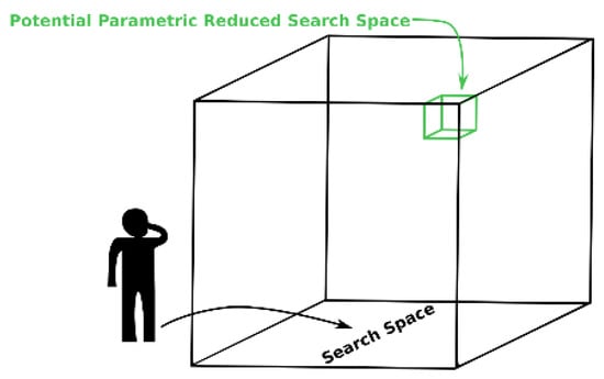
Figure 6.
Room analogy: The analyzer knows there is a resource and time constraint to scan the entire room for the potential optimal parametric match. However, based on previous experience (or previous research) he knows that there is a reduced search region that could lead to a good solution to the problem (not necessarily the optimal one). Source: own authors.
A lot of data, both from photovoltaic generation and climate, as well as the number of parameters from the machine learning models that can be combined, challenge the processing power of current computers, which is limited [40]. When referring to research involving computer simulation, there is usually many data and/or parameters involved. In order to mitigate the computational cost of the experiments of this work, the DOE was considered to reduce the parametric search space as it is an effective tool for this purpose [73].
The quality of reducing (or increasing) the depth of this search using DOE is measured in terms of confounding and is summarized in the experiment’s resolution. When there is a shortage of resources to carry out the experiments, in addition to choosing the levels of factors, the DOE allows the reduction of experimental runs, maintaining the statistical reliability [72] of these runs. As shown in Figure 7, this work considered level IV resolution, since at this level the main effects are considered without confusion with the interactions of two factors.

Figure 7.
Factorial design: experimental resolutions. This work considers 11 factors and 32 experimental runs. Source: own authors.
This research considered 11 factors in the experimental architecture, being separated into five factors related to the time series and six factors associated with the artificial neural network. The versatility of the experimental design, related to the essence of the photovoltaic generation prediction problem, allowed the choice of factors and their respective levels to be based on previous works [67], and one of these works also considers this object of study [37]. Knowing that there are numerous combinations of factors and that each factor has numerous levels, this search space becomes reduced when using DOE and, in this way, the analyzer can make changes in the factors or levels and understand the impact that this change has on the quality of the results. Table 3 summarizes each factor considered.
Table 3.
DOE Factors and Levels.
3.6. Mixture Design of Experiments (MDOE) for Defining the Ensemble Weights
Combining forecasts is to try to achieve better performance against the forecasters when considered individually [74]. The literature reports an empirical benefit of this combination in improving the forecast results [75]. Thus, this work uses Mixture DOE to combine the prediction results. Specifically, a mixing experiment considers finding the optimal proportions for each ingredient, that is, in the prediction problem, this proportion is identified by the weights and the factors represent the ingredients of this analogy.
Here, the combined value (which is taken as an answer) depends only on the weights (proportion of ingredients) and not just on the factors themselves. According to [76], the weights are non-negative, expressed as fractions of the mixtures, whose sum of all factors (ingredients) must be unity, as described in Equation (12):
Considering an example with three factors, or ingredients, there is a graphic representation of this arrangement as a triangle, as seen in Figure 8. The vertices are considered pure mixtures, because at these points the values of the weights of the other factors are null [14]. As the number of factors increases, the geometric representation also changes. For example, when considering four factors, the representation is given by a tetrahedron. Several factors greater than or equal to five are feasible, but there is no longer any possibility of visual representation.

Figure 8.
Mixture DOE example: Simplex Design with three factors. Source: own authors.
The metrics for evaluating and defining the weights is based on the mean absolute percentage error (MAPE), which has already been used in recent forecasting works [77], and on the root mean squared error (RMSE), which penalizes errors of greater magnitude, for comparison purposes. The error calculation is obtained as shown in Equation (13), for MAPE, and in Equation (14), for RMSE:
so that is the actual measurement value of the photovoltaic generation, is the predicted value and corresponds to the number of predicted points.
Figure 9 details the pseudocode that automates the prediction process described in the previous topics. The implementation of this algorithm took place through the Matlab software.
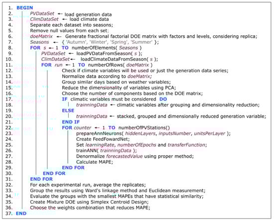
Figure 9.
Proposed pseudocode to automate the photovoltaic forecasting process. Source: own authors.
4. Case Study
Since, in Brazil, photovoltaic generation represents the largest share of renewable energy growth [78], this case study considered seventeen photovoltaic generation plants located in different regions of the country. The forecast was performed one day ahead, considering each season of the year, that is, at the end of the execution of the experiments, there were four forecasts for each generation plant (one for each season of the year). The forecast day was chosen randomly, given that the time interval of each generation plant did not always coincide (due to lack of data, for example).
The number of principal components, as a DOE factor, can be considered one of the key items in this research, as it leads to a reduction in the dimensionality of climatic variables. The levels vary between 2 and 3, which means that sometimes two components were used to train the model, and sometimes three components were used. The reduction in dimensionality implies a small loss of information. Thus, it is interesting to present the accumulated percentage of the variance at each level, for each city (generation plant).
From Figure 10, it is observed that the variance explanation of the climate variables, for each generation unit and considering each season of the year, is above 60%, with an approximate average of 75% of total explanation. For this graphical demonstration, the ‘MaxMin’ normalization process was used.

Figure 10.
Overview of the percentage of representation of the variance of climate variables considering two principal components. Source: own authors.
When considering three components, a natural increase in the explanation of the variance of climatic variables is perceived, which is shown in Figure 11. In this case, the percentage of explanation accumulated is above 75% for all generation plants and seasons, with an approximate average of 85% of explanation for all seasons. This means that if three components are used, there is a greater representation of the data set, which implies more information for adjustment and training of the forecast model. The idea is precisely to test, using the DOE statistical tool, if there is interference in the prediction results when an extra component is considered (or not).

Figure 11.
Overview of the percentage of representation of the variance of climate variables considering three principal components. Source: own authors.
4.1. Experiment Preparation Stage
All generation data were acquired from the pvoutput.org [41] repository, except for two photovoltaic generation plants, Machado and Passos, whose data were provided by the Federal Institute of Education, Science and Technology of South of Minas Gerais - IFSULDEMINAS. In order to facilitate the collection of this data, in an automated way, a script was implemented in the Java programming language that makes a request to the repository and download the data series with daily discretization, organizing them by generation plant. It is important to highlight a limitation that was observed in relation to the availability of data: there are more than 17 generation plants available in the repository, but many of them do not have the respective climate information, which was acquired from another database, the National Institute of Meteorology.–INMET [42].
The data collection stage was challenging, as much of this information had missing data, with noise and often without public access. Thus, since meteorological stations are dispersed throughout the Brazilian territory, they do not always coincide with being close to a given photovoltaic generation plant or even with the availability of climatic data, which reduces the number of experimental cases. In addition to the fact that climate data is not available for all generation plants (and vice versa), there is also the challenge of synchronizing measurement periods: often there is generation data for a range of dates, but there is no information weather forecast for the same period. When this happens, that time interval must be discarded. This is a reason why it was not possible to consider the same forecast day (respecting the season) for all generation units.
After eliminating missing data and synchronizing the date periods, the data was separated into seasons so that the training of the forecast model took place only with the specific data of that season. This process was considered because it is believed that each season of the year has its own characteristics, which can affect energy generation. For example, excess dust due to dry weather, or even the passage of clouds in periods of rain, can change the behavior and correlation of the data.
4.2. Day Ahead Forecasting by Season
The forecast is performed for each generation plant, taking one day ahead per season. With the DOE matrix, as in Table 4, all 32 experimental runs must be executed, which essentially translates the parametric variation in the search space. For each experimental run, the artificial neural network is re-initialized, in order to avoid interference in the results from one experimental run to another.
Table 4.
Structure of the DOE experimental matrix.
The experiments were performed in an automated way, whose algorithm was implemented in the Matlab® language. Thus, the average MAPE of each season of the year is included in Table 5, for all the experimental runs defined above.
Table 5.
Forecast results in terms of their mean errors (MAPEs) after each experimental run, separated by season.
Main effects plots allow the analyzer to visualize the parameters that may be influence the forecast positively (or negatively). Thus, the flexibility of analyzing forecasts by season, in terms of the parameters that most influence the entire process, stands out as one of the advantages of this methodology. Considering the average MAPE of each season of the year as a DOE response, the main effects of this execution can be identified. Here, the vertical axes of the graph show the average variation of the MAPE error, while the levels of each factor are distributed on the horizontal axes, i.e., in the case of photovoltaic forecasting, the smaller the error, the better the parameter level is. Figure 12 grouped four graphs, with Figure 12A showing the main effects of autumn, Figure 12B the main effects of winter, Figure 12C the main effects of spring and Figure 12D the main effects of summer.

Figure 12.
Main effects plot for each season, considering the average error of all seventeen generation plants. Source: own authors.
Autumn, represented by Figure 12A, presented interesting characteristics regarding the choice of some parameters, emphasizing the number of main components, which three adjusted well; the number of hidden layers was set to two; and the training algorithm was ‘Levenberg–Marquardt’. The other parameters, with a smaller variation in the error, such as the normalization method, verify that ‘minMax’ fits well; the use of climatic variables, in this case, had little effect on the results; the linkage method for day groupings was ‘complete’; the number of groups for cluster formation was four; the number of units per layer two; learning rate with little variation from one parameter to another; the number of epochs remained at 100; and the transfer function with little variation in error. Autumn was the only season of the year that differed from work expectations in terms of the use of climate variables.
On the other hand, winter, represented by Figure 12B, emphasizes the use of climatic variables in the forecast, with significant interference in the error variation. The normalization method that best fitted for this season was also ‘minMax’; the linkage method represented little variation in error; the number of clusters was four; the number of main components was three; the number of hidden layers two; the number of elements per layer hardly changes the error, as well as the number of epochs and the transfer function; the training algorithm was ‘Levenberg–Marquardt’.
In the same way, spring, represented by Figure 12C, promotes greater emphasis on the use of climate variables in the forecasting process, having good representation in error. In general, parameters like normalization method point to ‘minMax’, like the previous ones; hidden layers 2; and ‘Levenberg–Marquardt’ training algorithm. The other parameters exert little influence on the forecast error, considering this season of the year.
Last but not least, summer, represented by Figure 12D, also highlights the use of climate variables in the forecasting process, contributing to the reduction of error. As in the other seasons of the year, the normalization method was kept as ‘minMax’ as indicated to reduce the error. The binding method for forming the groups of similar days was ‘Ward’; The number of main components three; the number of neurons per layer 1.5 (according to the multiplication equation explained in the previous section); and symmetric ‘sigmoid’ transfer function. The other parameters not mentioned have little influence on the error when varied.
As expected from this investigation, most of the results indicate that the use of climatic variables, with at least three principal components in dimensionality reduction, contributes to the forecast error reduction.
4.3. Ensemble Forecasting
The motivation of the combination is to produce more accurate results than the best forecast components, considered individually. Thus, the combination of the prediction results used the Mixture DOE statistical tool to find the ideal weights so that the ensemble could be formed. Before, it was necessary to define how many factors (ingredients) would participate in this mixture. For this, the forecast results of each experimental run, initially processed, were classified according to the MAPE. Eight groups were chosen through cluster analysis, which uses the Ward linkage method with Euclidean distance. From these eight prediction groups, the one-way analysis of variance using Tukey’s comparison procedure was performed, so that only the group(s) with the smallest MAPEs, statistically different from the others, were chosen.
Figure 13 presents the interval plot that relates MAPEs by the groups. The group that statistically differed from the others and had the lowest MAPE was chosen. In the case of the forecast related to autumn, shown in Figure 13A, the results belonging to the ‘7’ group were chosen, which were three elements. The winter season, indicated by Figure 13B, revealed two statistically equal groups with lower MAPE, ‘4’ and ‘7’, with the total of these two groups having four elements. Spring identified the group numbered ‘2’ in Figure 13C, which had five elements favorable to the combination, and summer classified the group numbered ‘8’ in Figure 13D as the group with the lowest MAPE, having three elements. Thus, the formation of the Mixture DOE is a function of the number of elements (factors or ingredients) to be combined. In this case, each factor represents the weight that optimizes the combination and aims to reduce the total MAPE.

Figure 13.
Main effects plot for each season, considering the average error of all seventeen generation plants. Source: own authors.
Table 6 summarizes the weight combinations for three elements. Here, the average MAPEs are presented for the autumn and summer seasons. Specifically, for autumn, the weights that best fitted the forecasts were (0.333, 0.333, 0.333) with a mean MAPE of 9.29% and a standard deviation of 7.23. For the summer, the combination of weights that best fitted the forecasts was (0.00, 0.50, 0.50), with a mean MAPE of 10.45% and a standard deviation of 7.34.
Table 6.
Mixture DOE arrangement considering three elements to be combined. Results for autumn and winter are listed.
Table 7 lists the combinations of weights for the day’s forecast whose season is winter. This table presents four elements that participate in this combined forecast. The weights that make this mixture ideal are given by (0.00, 0.00, 0.50, 0.50) with an average MAPE of 9.11% and standard deviation of 5.55.
Table 7.
Mixture DOE arrangement considering four elements to be combined. Results for winter are listed.
Table 8 lists the weights for the spring day forecast. Since there are now five elements to combine, the table naturally grows. The ideal combination of these elements is given by the weights (0.00, 0.00, 0.333, 0.333, 0.333) with a mean MAPE of 6.75% and a standard deviation of 6.47.
Table 8.
Mixture DOE arrangement considering four elements to be combined. Results for spring are listed.
When one of the weights is null, it indicates that that respective element does not contribute to the formation of the ensemble and can be discarded, since the multiplication by zero is zero. A geometric representation of each combination can be visualized using the triangle (for three elements) and the tetrahedron (for four elements). Five or more elements are feasible, but the geometric representation is more difficult to see. From this perspective, Figure 14 presents the representation of the ideal point of a combination of forecasts for each season of the year, except spring (which has five weights). Autumn and summer appear in Figure 14A,C, respectively, through the triangle and winter in Figure 14B, through the tetrahedron.
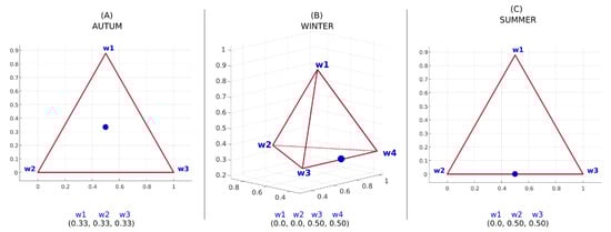
Figure 14.
Adjusted weight combination that configures the smallest forecast errors for the seventeen generation plants, separated by season: (A) Autumn—(0.33, 0.33, 0.33); (B) Winter—(0.0, 0.0, 0.5, 0.5); (C) Summer—(0.0, 0.5, 0.5) and spring, which is not plotted because the combination elements contained 5 factors (hard to see): (0.0, 0.0, 0.33, 0.33, 0.33). Source: own authors.
As each generation plant has a photovoltaic generation capacity different from the others, forecasted values may vary in scale. This phenomenon is also observed during the calculation of the RMSE, which penalizes higher errors in its metric. Therefore, the actual values and the predicted values are shown in Table 9. The lowest values in scale are observed in Machado and Passos, respectively, and the highest values in scale are observed in Ituporanga.
Table 9.
Predicted values and actual generation values for each generation plant, grouped by season.
These forecasted values were compiled into a chart (Figure 15) where each red dot represents a forecast value for one day ahead for each generation plant. The yellow dots indicate the actual generation values. Charts are grouped by season.
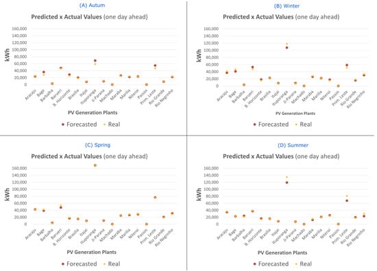
Figure 15.
Predicted versus actual values plot, grouped by season.
The map in Figure 16 displays the final, combined forecast for each photovoltaic generation plant and its respective MAPEs. The highest numerically observed values of the MAPEs were 28.4% (autumn—Bagé) and 23.6% (summer—Rio Negrinho). On the contrary, the numerically lower values for each season were 0.1% (winter—Machado and spring—Ituporanga), 0.5% (autumn—Niterói and spring—Niterói), 0.6% (winter—Passos) and 0.9% (summer—Bagé). The season with the lowest overall average was spring, possibly because it is less subject to uncontrollable factors, such as movement of clouds, dust, etc.

Figure 16.
Error intensity map by season: the results displayed are the minimum MAPEs found for each generation plant, after the process of combining the results. The maps were generated using the JavaScript language, through the open source library jQuery MAPAEL [79]. Source: own authors.
There are studies that use different databases of regions with different characteristics from each other. For purposes of comparison with the works developed in the existing literature, the results that use the MAPE metric associated with machine learning models and hybrid models are perceived in an average error range of 10% to 15%, approximately. These values were obtained from [80], which investigated about 180 papers related to photovoltaic generation forecast published in the last fifteen years. Therefore, the results found in the case study of this work were optimized from the average error of seventeen generation plants, analyzed together. These results are consistent with the study proposed by [80].
5. Conclusions
This work presented a photovoltaic generation prediction methodology, whose versatility allows the analyzer to identify the parameters that most interfere with the results. As the main contribution, the reduction of dimensionality of meteorological data in this process is highlighted. Keeping the levels of explanation of the variables, the reduction of the data set using PCA explained the variance of seventeen climatic variables, reducing them to two or three variables, with a satisfactory degree of average explanation around 75–85%.
It was experimentally found that the combined forecast produced better results when compared to the best forecasters, considered individually. The case study covered 17 generation plants located in different regions of the Brazilian territory, and the parametric evaluation considered all these plants together. The smallest mean errors found for the combined seasonal forecast were 9.29% and standard deviation 7.23 for autumn, 10.45% and standard deviation 7.34 for summer, 9.11% and standard deviation 5.55 for winter and 6.75% and standard deviation 6.47 for spring. Since the amount of climate data and photovoltaic generation tends to increase, future work should explore other heuristic methods besides ANNs to verify the fit to the data, which can be different for different regions.
Therefore, this article presents a methodological proposal that promotes advances in the studies and practice of adopting one-step-ahead prediction models based on machine learning for short-term predictions. Specifically, the one-day-ahead time horizon was considered. Faced with the challenge of guaranteeing greater precision, the proposed model brings contributions insofar as it reduces training time and computational costs, and optimizes hyperparameters of the algorithms and models complex temporal characteristics.
Furthermore, the choice of forecasting methods based on artificial intelligence and not strictly on traditional statistical methods allowed the reproduction of non-linear behaviors more accurately. It is also worth mentioning the theoretical contribution of this research in several fields of knowledge. The multidisciplinary bias of the study, involving statistics, engineering and data science, brings advances in different areas.
Limitations of this study include, since heuristic methods are considered: there is no guarantee of obtaining the optimal forecasting solution, as well as uncontrollable factors (such as dust deposited on the panels, damaged sensors, lack of data, etc.) that can lead to inconsistent predictions.
Author Contributions
Conceptualization, M.O.M. and P.P.B.; methodology, M.O.M. and A.C.Z.d.S.; software, M.O.M. and T.O.; validation, T.O. and P.P.B.; investigation, B.D.B.; writing—original draft preparation, B.M.K.; writing—review and editing, A.C.Z.d.S.; visualization, B.D.B.; supervision, P.P.B. All authors have read and agreed to the published version of the manuscript.
Funding
This research received no external funding.
Data Availability Statement
The data presented in this study are available on request from the corresponding author. The data are not publicly available due to statistical analysis and pre-processing techniques needed.
Acknowledgments
This work has been supported in part by the following Brazilian Research Agencies: Federal Institute of Education, Science and Technology—South of Minas Gerais - IFSULDEMINAS, UNIFEI, UNICAMP, FAPESP, FAPEMIG, INERGE, CAPES, CNPq, FINEP. One author is funded by grant #2021/11380-5, CPTEn-FAPESP.
Conflicts of Interest
The authors declare no conflict of interest.
References
- Zeren, F.; Akkuş, H.T. The relationship between renewable energy consumption and trade openness: New evidence from emerging economies. Renew. Energy 2019, 147, 322–329. [Google Scholar] [CrossRef]
- Du, E.; Zhang, N.; Hodge, B.-M.; Wang, Q.; Lu, Z.; Kang, C.; Kroposki, B.; Xia, Q. Operation of a High Renewable Penetrated Power System with CSP Plants: A Look-Ahead Stochastic Unit Commitment Model. IEEE Trans. Power Syst. 2018, 34, 140–151. [Google Scholar] [CrossRef]
- Wang, Q.; Hobbs, W.B.; Tuohy, A.; Bello, M.; Ault, D.J. Evaluating Potential Benefits of Flexible Solar Power Generation in the Southern Company System. IEEE J. Photovolt. 2021, 12, 152–160. [Google Scholar] [CrossRef]
- Yousefi, M.; Hajizadeh, A.; Soltani, M.N. A Comparison Study on Stochastic Modeling Methods for Home Energy Management Systems. IEEE Trans. Ind. Inform. 2019, 15, 4799–4808. [Google Scholar] [CrossRef]
- Sobri, S.; Koohi-Kamali, S.; Rahim, N.A. Solar photovoltaic generation forecasting methods: A review. Energy Convers. Manag. 2018, 156, 459–497. [Google Scholar] [CrossRef]
- Rodrigues, B.K.F.; Gomes, M.; Santanna, A.M.O.; Barbosa, D.; Martinez, L. Modelling and forecasting for solar irradiance from solarimetric station. IEEE Lat. Am. Trans. 2021, 20, 250–258. [Google Scholar] [CrossRef]
- Hossain, M.; Mekhilef, S.; Danesh, M.; Olatomiwa, L.; Shamshirband, S. Application of extreme learning machine for short term output power forecasting of three grid-connected PV systems. J. Clean. Prod. 2017, 167, 395–405. [Google Scholar] [CrossRef]
- Zhen, Z.; Liu, J.; Zhang, Z.; Wang, F.; Chai, H.; Yu, Y.; Lu, X.; Wang, T.; Lin, Y. Deep Learning Based Surface Irradiance Mapping Model for Solar PV Power Forecasting Using Sky Image. IEEE Trans. Ind. Appl. 2020, 56, 3385–3396. [Google Scholar] [CrossRef]
- Cui, J.; Liu, S.; Yang, J.; Ge, W.; Zhou, X.; Wang, A. A Load Combination Prediction Algorithm Considering Flexible Charge and Discharge of Electric Vehicles. In Proceedings of the 2019 IEEE 10th International Symposium on Power Electronics for Distributed Generation Systems (PEDG), Xi’an, China, 3–6 June 2019; pp. 711–716. [Google Scholar] [CrossRef]
- Gomez-Quiles, C.; Asencio-Cortes, G.; Gastalver-Rubio, A.; Martinez-Alvarez, F.; Troncoso, A.; Manresa, J.; Riquelme, J.C.; Riquelme-Santos, J.M. A Novel Ensemble Method for Electric Vehicle Power Consumption Forecasting: Application to the Spanish System. IEEE Access 2019, 7, 120840–120856. [Google Scholar] [CrossRef]
- Zheng, Y.; Song, Y.; Hill, D.J.; Meng, K. Online Distributed MPC-Based Optimal Scheduling for EV Charging Stations in Distribution Systems. IEEE Trans. Ind. Inform. 2018, 15, 638–649. [Google Scholar] [CrossRef]
- Mishra, S.; Tripathy, L.; Satapathy, P.; Dash, P.K.; Sahani, N. An Efficient Machine Learning Approach for Accurate Short Term Solar Power Prediction. In Proceedings of the 2020 International Conference on Computational Intelligence for Smart Power System and Sustainable Energy (CISPSSE), Keonjhar, India, 29–31 July 2020; pp. 1–6. [Google Scholar] [CrossRef]
- Yao, T.; Wang, J.; Wu, H.; Zhang, P.; Li, S.; Xu, K.; Liu, X.; Chi, X. Intra-Hour Photovoltaic Generation Forecasting Based on Multi-Source Data and Deep Learning Methods. IEEE Trans. Sustain. Energy 2021, 13, 607–618. [Google Scholar] [CrossRef]
- Montgomery, D.C. Design and Analysis of Experiments; John Wiley & sons: Hoboken, NJ, USA, 2017. [Google Scholar]
- Galicia, A.; Talavera-Llames, R.; Troncoso, A.; Koprinska, I.; Martínez-Álvarez, F. Multi-step forecasting for big data time series based on ensemble learning. Knowl.-Based Syst. 2018, 163, 830–841. [Google Scholar] [CrossRef]
- Lin, J.; Ma, J.; Zhu, J. A Privacy-Preserving Federated Learning Method for Probabilistic Community-Level Behind-the-Meter Solar Generation Disaggregation. IEEE Trans. Smart Grid 2021, 13, 268–279. [Google Scholar] [CrossRef]
- Huang, X.; Li, Q.; Tai, Y.; Chen, Z.; Liu, J.; Shi, J.; Liu, W. Time series forecasting for hourly photovoltaic power using conditional generative adversarial network and Bi-LSTM. Energy 2022, 246, 123403. [Google Scholar] [CrossRef]
- Zhou, Y.; Wang, J.; Li, Z.; Lu, H. Short-term photovoltaic power forecasting based on signal decomposition and machine learning optimization. Energy Convers. Manag. 2022, 267, 115944. [Google Scholar] [CrossRef]
- Costa, R.L.D.C. Convolutional-LSTM networks and generalization in forecasting of household photovoltaic generation. Eng. Appl. Artif. Intell. 2022, 116, 105458. [Google Scholar] [CrossRef]
- Zhang, C.; Peng, T.; Nazir, M.S. A novel integrated photovoltaic power forecasting model based on variational mode decomposition and CNN-BiGRU considering meteorological variables. Electr. Power Syst. Res. 2022, 213, 108796. [Google Scholar] [CrossRef]
- Si, Z.; Yang, M.; Yu, Y.; Ding, T. Photovoltaic power forecast based on satellite images considering effects of solar position. Appl. Energy 2021, 302, 117514. [Google Scholar] [CrossRef]
- Wang, Z.; Wang, C.; Cheng, L.; Li, G. An approach for day-ahead interval forecasting of photovoltaic power: A novel DCGAN and LSTM based quantile regression modeling method. Energy Rep. 2022, 8, 14020–14033. [Google Scholar] [CrossRef]
- Gu, B.; Shen, H.; Lei, X.; Hu, H.; Liu, X. Forecasting and uncertainty analysis of day-ahead photovoltaic power using a novel forecasting method. Appl. Energy 2021, 299, 117291. [Google Scholar] [CrossRef]
- Dai, Y.; Wang, Y.; Leng, M.; Yang, X.; Zhou, Q. LOWESS smoothing and Random Forest based GRU model: A short-term photovoltaic power generation forecasting method. Energy 2022, 256, 124661. [Google Scholar] [CrossRef]
- Borunda, M.; Ramírez, A.; Garduno, R.; Ruíz, G.; Hernandez, S.; Jaramillo, O.A. Photovoltaic Power Generation Forecasting for Regional Assessment Using Machine Learning. Energies 2022, 15, 8895. [Google Scholar] [CrossRef]
- Khan, M.A.; Ashraf, B.; Ali, H.; Khan, S.; Baig, D.-E. Output Power Prediction of a Photovoltaic Module through Artificial Neural Network. IEEE Access 2022, 10, 116160–116166. [Google Scholar] [CrossRef]
- Niccolai, A.; Ogliari, E.; Nespoli, A.; Zich, R.; Vanetti, V. Very Short-Term Forecast: Different Classification Methods of the Whole Sky Camera Images for Sudden PV Power Variations Detection. Energies 2022, 15, 9433. [Google Scholar] [CrossRef]
- Yin, L.; Cao, X.; Liu, D. Weighted fully-connected regression networks for one-day-ahead hourly photovoltaic power forecasting. Appl. Energy 2023, 332, 120527. [Google Scholar] [CrossRef]
- Zhao, E.; Sun, S.; Wang, S. New developments in wind energy forecasting with artificial intelligence and big data: A scientometric insight. J. Inf. Technol. Data Manag. 2022, 5, 84–95. [Google Scholar] [CrossRef]
- Peng, L.; Wang, L.; Xia, D.; Gao, Q. Effective energy consumption forecasting using empirical wavelet transform and long short-term memory. Energy 2022, 238, 121756. [Google Scholar] [CrossRef]
- Arvanitidis, A.I.; Bargiotas, D.; Daskalopulu, A.; Kontogiannis, D.; Panapakidis, I.P.; Tsoukalas, L.H. Clustering Informed MLP Models for Fast and Accurate Short-Term Load Forecasting. Energies 2022, 15, 1295. [Google Scholar] [CrossRef]
- Haghighat, F. Predicting the trend of indicators related to COVID-19 using the combined MLP-MC model. Chaos Solitons Fractals 2021, 152, 111399. [Google Scholar] [CrossRef]
- Yuan, F.; Zhang, Z.; Fang, Z. An effective CNN and Transformer complementary network for medical image segmentation. Pattern Recognit. 2023, 136, 109228. [Google Scholar] [CrossRef]
- Satyanarayana, G.; Deshmukh, P.; Das, S.K. Vehicle detection and classification with spatio-temporal information obtained from CNN. Displays 2022, 75, 102294. [Google Scholar] [CrossRef]
- Khalifani, S.; Darvishzadeh, R.; Azad, N.; Rahmani, R.S. Prediction of sunflower grain yield under normal and salinity stress by RBF, MLP and, CNN models. Ind. Crop. Prod. 2022, 189, 115762. [Google Scholar] [CrossRef]
- Yang, K.; Wang, Y.; Li, M.; Li, X.; Wang, H.; Xiao, Q. Modeling topological nature of gas–liquid mixing process inside rectangular channel using RBF-NN combined with CEEMDAN-VMD. Chem. Eng. Sci. 2023, 267, 118353. [Google Scholar] [CrossRef]
- Moreira, M.; Balestrassi, P.; Paiva, A.; Ribeiro, P.; Bonatto, B. Design of experiments using artificial neural network ensemble for photovoltaic generation forecasting. Renew. Sustain. Energy Rev. 2021, 135, 110450. [Google Scholar] [CrossRef]
- Srivastava, S.; Lessmann, S. A comparative study of LSTM neural networks in forecasting day-ahead global horizontal irradiance with satellite data. Sol. Energy 2018, 162, 232–247. [Google Scholar] [CrossRef]
- Aksu, G.; Güzeller, C.O.; Eser, M.T. The Effect of the Normalization Method Used in Different Sample Sizes on the Success of Artificial Neural Network Model. Int. J. Assess. Tools Educ. 2019, 6, 170–192. [Google Scholar] [CrossRef]
- Massaoudi, M.; Chihi, I.; Abu-Rub, H.; Refaat, S.S.; Oueslati, F.S. Convergence of Photovoltaic Power Forecasting and Deep Learning: State-of-Art Review. IEEE Access 2021, 9, 136593–136615. [Google Scholar] [CrossRef]
- PVOutput 2021. Available online: https://www.pvoutput.org/ (accessed on 1 December 2021).
- INMET Meteorological Database. Available online: https://portal.inmet.gov.br/ (accessed on 13 December 2021).
- Donaldson, D.L.; Piper, D.M.; Jayaweera, D. Temporal Solar Photovoltaic Generation Capacity Reduction from Wildfire Smoke. IEEE Access 2021, 9, 79841–79852. [Google Scholar] [CrossRef]
- Zhang, X.; Li, Y.; Lu, S.; Hamann, H.F.; Hodge, B.-M.S.; Lehman, B. A Solar Time Based Analog Ensemble Method for Regional Solar Power Forecasting. IEEE Trans. Sustain. Energy 2019, 10, 268–279. [Google Scholar] [CrossRef]
- Alaraj, M.; Kumar, A.; Alsaidan, I.; Rizwan, M.; Jamil, M. Energy Production Forecasting from Solar Photovoltaic Plants Based on Meteorological Parameters for Qassim Region, Saudi Arabia. IEEE Access 2021, 9, 83241–83251. [Google Scholar] [CrossRef]
- Urolagin, S.; Sharma, N.; Datta, T.K. A combined architecture of multivariate LSTM with Mahalanobis and Z-Score transformations for oil price forecasting. Energy 2021, 231, 120963. [Google Scholar] [CrossRef]
- De Almeida, F.A.; De Mello, L.G.; Romao, E.L.; Gomes, G.F.; Gomes, J.H.D.F.; De Paiva, A.P.; Filho, J.M.; Balestrassi, P.P. A PCA-Based Consistency and Sensitivity Approach for Assessing Linkage Methods in Voltage Sag Studies. IEEE Access 2021, 9, 84871–84885. [Google Scholar] [CrossRef]
- De Luca, G.; Zuccolotto, P. Hierarchical time series clustering on tail dependence with linkage based on a multivariate copula approach. Int. J. Approx. Reason. 2021, 139, 88–103. [Google Scholar] [CrossRef]
- Tokuda, E.K.; Comin, C.H.; Costa, L.D.F. Revisiting agglomerative clustering. Phys. A Stat. Mech. Appl. 2022, 585, 126433. [Google Scholar] [CrossRef]
- de Almeida, F.A.; Romão, E.L.; Gomes, G.F.; Gomes, J.H.D.F.; de Paiva, A.P.; Filho, J.M.; Balestrassi, P.P. Combining machine learning techniques with Kappa–Kendall indexes for robust hard-cluster assessment in substation pattern recognition. Electr. Power Syst. Res. 2022, 206, 107778. [Google Scholar] [CrossRef]
- Xia, J.; Zhang, Y.; Song, J.; Chen, Y.; Wang, Y.; Liu, S. Revisiting Dimensionality Reduction Techniques for Visual Cluster Analysis: An Empirical Study. IEEE Trans. Vis. Comput. Graph. 2022, 28, 529–539. [Google Scholar] [CrossRef]
- Ahmadi, M.; Samet, H.; Ghanbari, T. A New Method for Detecting Series Arc Fault in Photovoltaic Systems Based on the Blind-Source Separation. IEEE Trans. Ind. Electron. 2020, 67, 5041–5049. [Google Scholar] [CrossRef]
- Johnson, R.A.; Wichern, D.W. Applied Multivariate Statistical Analysis; Pearson Prentice Hall: Hoboken, NJ, USA, 2007. [Google Scholar]
- Rencher, A.C. Methods of Multivariate Analysis; Wiley: Hoboken, NJ, USA, 2003. [Google Scholar]
- Ge, L.; Xian, Y.; Yan, J.; Wang, B.; Wang, Z. A Hybrid Model for Short-term PV Output Forecasting Based on PCA-GWO-GRNN. J. Mod. Power Syst. Clean Energy 2020, 8, 1268–1275. [Google Scholar] [CrossRef]
- Wang, L.; Wang, S.; Yuan, Z.; Peng, L. Analyzing potential tourist behavior using PCA and modified affinity propagation clustering based on Baidu index: Taking Beijing city as an example. Data Sci. Manag. 2021, 2, 12–19. [Google Scholar] [CrossRef]
- Rudnik, K.; Hnydiuk-Stefan, A.; Kucińska-Landwójtowicz, A.; Mach, Ł. Forecasting Day-Ahead Carbon Price by Modelling Its Determinants Using the PCA-Based Approach. Energies 2022, 15, 8057. [Google Scholar] [CrossRef]
- Khelil, C.K.M.; Amrouche, B.; Kara, K.; Chouder, A. The impact of the ANN’s choice on PV systems diagnosis quality. Energy Convers. Manag. 2021, 240, 114278. [Google Scholar] [CrossRef]
- Dhimish, M.; Holmes, V.; Mehrdadi, B.; Dales, M. Comparing Mamdani Sugeno fuzzy logic and RBF ANN network for PV fault detection. Renew. Energy 2018, 117, 257–274. [Google Scholar] [CrossRef]
- Wang, J.; Zhou, Y.; Li, Z. Hour-ahead photovoltaic generation forecasting method based on machine learning and multi objective optimization algorithm. Appl. Energy 2022, 312, 118725. [Google Scholar] [CrossRef]
- Kim, J.; Oh, H.; Choi, J.K. Learning based cost optimal energy management model for campus microgrid systems. Appl. Energy 2022, 311, 118630. [Google Scholar] [CrossRef]
- Lin, Y.; Li, B.; Moiser, T.M.; Griffel, L.M.; Mahalik, M.R.; Kwon, J.; Alam, S.M.S. Revenue prediction for integrated renewable energy and energy storage system using machine learning techniques. J. Energy Storage 2022, 50, 104123. [Google Scholar] [CrossRef]
- Yahya, Z.; Imane, S.; Hicham, H.; Ghassane, A.; Safia, E.B.-I. Applied imagery pattern recognition for photovoltaic modules’ inspection: A review on methods, challenges and future development. Sustain. Energy Technol. Assess. 2022, 52, 102071. [Google Scholar] [CrossRef]
- Kotu, V.; Deshpande, B. Chapter 4-Classification. In Data Science, 2nd ed.; Morgan Kaufmann: Burlington, MA, USA, 2019; pp. 65–163. [Google Scholar] [CrossRef]
- Mahfoud, S.; Derouich, A.; EL Ouanjli, N.; EL Mahfoud, M. Enhancement of the Direct Torque Control by using Artificial Neuron Network for a Doubly Fed Induction Motor. Intell. Syst. Appl. 2022, 13, 200060. [Google Scholar] [CrossRef]
- Zekić-Sušac, M.; Has, A.; Knežević, M. Predicting energy cost of public buildings by artificial neural networks, CART, and random forest. Neurocomputing 2021, 439, 223–233. [Google Scholar] [CrossRef]
- Balestrassi, P.; Popova, E.; Paiva, A.; Lima, J.M. Design of experiments on neural network’s training for nonlinear time series forecasting. Neurocomputing 2009, 72, 1160–1178. [Google Scholar] [CrossRef]
- Pontes, F.J.; Amorim, G.F.; Balestrassi, P.P.; Paiva, A.P.; Ferreira, J.R. Design of experiments and focused grid search for neural network parameter optimization. Neurocomputing 2016, 186, 22–34. [Google Scholar] [CrossRef]
- Chu, X.; Luo, Y.; Wang, J.; Guo, W.; Wu, F.; Wang, W.; Li, W. Fast Multiple Edge Response Method Based on the Design of Experiment and Machine Learning. IEEE Microw. Wirel. Compon. Lett. 2021, 31, 521–524. [Google Scholar] [CrossRef]
- Sbayti, M.; Ghiotti, A.; Bahloul, R.; BelhadjSalah, H.; Bruschi, S. Effective strategies of metamodeling and optimization of hot incremental sheet forming process of Ti6Al4Vartificial hip joint component. J. Comput. Sci. 2022, 101595. [Google Scholar] [CrossRef]
- Antony, J. 6-Full Factorial Designs. In Design of Experiments for Engineers and Scientists, 2nd ed.; Elsevier: Oxford, UK, 2014; pp. 63–85. [Google Scholar] [CrossRef]
- Jankovic, A.; Chaudhary, G.; Goia, F. Designing the design of experiments (DOE) – An investigation on the influence of different factorial designs on the characterization of complex systems. Energy Build. 2021, 250, 111298. [Google Scholar] [CrossRef]
- Khan, K.; Shukla, S.; Singh, B. Improved Performance Design Realization of Fractional kW Induction Motor with Predictive Current Control for Water Pumping. IEEE Trans. Ind. Appl. 2020, 56, 4575–4587. [Google Scholar] [CrossRef]
- Kourentzes, N.; Barrow, D.; Petropoulos, F. Another look at forecast selection and combination: Evidence from forecast pooling. Int. J. Prod. Econ. 2019, 209, 226–235. [Google Scholar] [CrossRef]
- Qian, W.; Rolling, C.A.; Cheng, G.; Yang, Y. Combining forecasts for universally optimal performance. Int. J. Forecast. 2022, 38, 193–208. [Google Scholar] [CrossRef]
- Cornell, J.A. Experiments with Mixtures: Designs, Models, and the Analysis of Mixture Data; Wiley: Hoboken, NJ, USA, 2011. [Google Scholar]
- Niu, D.; Yu, M.; Sun, L.; Gao, T.; Wang, K. Short-term multi-energy load forecasting for integrated energy systems based on CNN-BiGRU optimized by attention mechanism. Appl. Energy 2022, 313, 118801. [Google Scholar] [CrossRef]
- Rigo, P.D.; Siluk, J.C.M.; Lacerda, D.P.; Spellmeier, J.P. Competitive business model of photovoltaic solar energy installers in Brazil. Renew. Energy 2022, 181, 39–50. [Google Scholar] [CrossRef]
- Brouté, V. jQuery Mapael-Dynamic vector maps. Available online: https://github.com/neveldo/jQuery-Mapael (accessed on 13 December 2021).
- Nguyen, T.N.; Müsgens, F. What drives the accuracy of PV output forecasts? Appl. Energy 2022, 323, 119603. [Google Scholar] [CrossRef]


Disclaimer/Publisher’s Note: The statements, opinions and data contained in all publications are solely those of the individual author(s) and contributor(s) and not of MDPI and/or the editor(s). MDPI and/or the editor(s) disclaim responsibility for any injury to people or property resulting from any ideas, methods, instructions or products referred to in the content. |
© 2022 by the authors. Licensee MDPI, Basel, Switzerland. This article is an open access article distributed under the terms and conditions of the Creative Commons Attribution (CC BY) license (https://creativecommons.org/licenses/by/4.0/).