Cooling Optimization Strategy for a 6s4p Lithium-Ion Battery Pack Based on Triple-Step Nonlinear Method

Abstract

In a battery cooling system, by adopting a cooling optimization control strategy, the battery temperature under different external environments and load currents can be adjusted to ensure performance and safety. In this study, two modes of the thermal management system are established for the 6s4p (six serial and four parallel batteries in a stage) battery pack. A single particle model, considering battery aging, is adopted for the battery. Furthermore, a cooling optimization control strategy for the battery is proposed based on the triple-step nonlinear method, and then the optimization effect is validated under two C-rate charge–discharge cycles, NEDC cycles, and US06 cycles. Moreover, an extended PID control strategy is constructed and compared with the triple-step nonlinear method. A comparison of pump power, thermal behavior, and aging performance indicate parallel cooling is more advantageous. This verifies the validity of the triple-step nonlinear method and shows its advantages over the extended PID method. The present study provides a method to investigate the thermal behavior and aging performance of a battery pack in a BTM system, and fills in the research gaps in the cooling optimization control strategy for battery packs.

1. Introduction

The vigorous development and widespread introduction of electric vehicles (EVs) have placed higher requirements on the driving endurance and safety performance of EVs [1]. Lithium-ion batteries (LIBs) are widely used in the automobile industry and in energy storage due to their high energy density [2,3]. However, the size and number of batteries cannot be increased indefinitely due to the limitations in vehicle space. Therefore, increasing the energy density and power density of batteries has become a priority to improve the driving endurance of EVs [4]. As the energy density and power density of the battery increase, the heat generation also increases. This requires an effective cooling method to dissipate the large amount of heat accumulated inside the battery over time [5]. Otherwise, the battery temperature will rise sharply and the battery capacity will continuously decline. In severe cases, it may even lead to thermal runaway or fire and explosion [6,7]. In addition, there are also many studies on the generation of LIBs for systematic research [8,9].

Many investigations have been conducted to better understand and improve battery performance. Some researchers have established battery thermal management (BTM) systems to control the temperature [10,11,12,13]. Studies of BTM system include air-cooling [14,15], liquid-cooling [16,17], phase-change material cooling [18,19], heat pipe-cooling [20,21], and cooling systems combined with the aforementioned methods [22,23,24]. Other researchers have studied the internal aging mechanism and battery aging to lay a foundation for the design of BTM systems [25,26]. Birkl et al. [27] summarized the causes, mechanisms, modes, and effects of battery aging. The causes trigger the mechanisms, and the mechanisms contribute to the modes of aging. The aging modes can be divided into three categories: loss of lithium inventory, loss of active material of the negative electrode (NE), loss of active material of the and positive electrode (PE). These modes contribute to the aging of the battery and the battery capacities decline. A widely studied aging mechanism is the formation of a solid electrolyte interface (SEI) [28,29]. The charge–discharge rate (C-rate, defined as the measurement of the charge and discharge speed, which equals the current required for the battery to charge or discharge its capacity in a specified time) and ambient temperature are generally considered to be the important factors affecting the aging mechanisms [30,31]. Many experimental studies on battery aging and thermal management systems have been conducted. However, experiments on thermal management systems are complicated and time-consuming, especially when multiple charge–discharge cycle tests are required to consider battery aging. Numerical simulations of BTM systems under different EV-related cycle conditions are efficient and low-cost as they can reduce the number of experiments [32].

The difficulty in the simulation of LIBs is related to their multi-domain and multi-physics characteristics. Therefore, various battery models have been used to characterize the performance of LIBs, and these models have been developed to study electrochemical performance [33], aging [34], and even thermal runaway [35]. The single particle (SP) model is a commonly-used reduced-order electrochemical model, which was proposed by Haran et al. [36] based on the pseudo-two-dimensional model of Doyle–Fuller–Newman [37]. In the SP model, it is assumed that both electrodes are composed of multiple spherical particles of uniform size and the current is uniformly distributed on both electrodes. Therefore, each electrode can be approximated as a single spherical particle. The SP model is described by a set of ordinary differential equations, and it is derived directly from a comprehensive electrochemical model, thus explicitly preserving many important battery properties with high computational efficiency. The disadvantage of the SP model is that the electrolyte physics and degradation are not considered, so the accuracy at high C-rates is affected. Many researchers have established advanced SP models to address this deficiency.

Rahimian et al. [38] compared the SP model with a semi-empirical equivalent circuit model to predict battery voltages under constant current charge and discharge for different LIB datasets. The results showed that the SP model outperforms the equivalent circuit model in its predictive power for all datasets, while the computation time of both models was on the same order of magnitude. Li et al. [39] developed an aging model based on the SP model considering SEI layer formation and the stress due to the volume expansion of the particles in the active material. The Li-ion loss model due to SEI layer formation was integrated with an advanced SP model that incorporates electrolytic physics. This model can rapidly predict capacity fade and voltage profile changes as a function of cycle number and temperature with high accuracy. Richardson et al. [40] compared the SP model and the Doyle–Fuller–Newman model for different electrode materials, including lithium nickel manganese cobalt oxide, graphite, and lithium iron phosphate (LFP). Motivated by these differences, correction terms for the SP model were derived. Incorporating this into the SP model resulted in a corrected SP model that was significantly more accurate than the original SP model. Ren et al. [41] proposed an extended SP model with higher accuracy. Based on this model, a new state of charge (SOC) closed-loop estimation algorithm model was constructed. The results showed that the extended SP model can effectively simulate the performance of the battery, and the closed-loop SOC estimation algorithm can correct the initial SOC error without increasing the computational complexity.

In the modeling of the BTM system, in addition to the selection and optimization of a battery model to ensure the accuracy of the simulation, it is also necessary to select an appropriate cooling method. As mentioned above, the current main cooling methods for batteries are air cooling and liquid cooling. However, the research on battery cooling mainly focuses on the structural design and analysis of factors, and research on the optimization and control strategy of battery cooling is still in its infancy. Ji et al. [42] proposed an active temperature control method to equalize the temperature distribution of the batteries by adjusting the coolant flow rate. The optimal cooling flow rate was determined by setting different coolant flow rates to find the lowest battery temperature. This method is complex and costly and is not suitable for complicated operating conditions. Zhu et al. [43] presented a finite-set-based model predictive control strategy for the BTM in hybrid EVs and verified the strategy under different cycle conditions. However, due to a large amount of computational data and high hardware requirements, this optimization process using dynamic programming algorithms was complicated. Ma et al. [44] proposed a cooling optimization strategy for LIBs based on the triple-step nonlinear method and compared the strategy with the PID method under NEDC and US06 cycle conditions. The results showed that the proposed method ensures a stable operating temperature and cooling process of LIBs. Ma et al. [45] further proposed a nonlinear model predictive control to optimize the cooling process of the battery module. The simulation results showed that the nonlinear model predictive control method ensured that the battery works near a target temperature under different working conditions. However, the battery model used in these studies was a lumped thermal model, which cannot reflect the electrochemical performance and aging of the battery. Moreover, the proposed cooling optimization strategies have only been used for the verification of a single battery, and the effect of applying a battery pack has not been studied.

As mentioned above, the advanced SP model is rarely used in the modeling of a BTM system and the cooling optimization strategy has been verified only for a single battery, which limits the application in real scenarios. Therefore, the gaps and deficiencies that are present in the literature are investigated in this study. First, a one-dimensional thermal management model of the 6s4p (six serial and four parallel batteries in a stage) battery pack is established for the first time based on our previous work [32]. The SP model, with a consideration of battery aging, is adopted to the 6s4p battery pack, so the electrochemical performance and degradation of each cell can be obtained more accurately. Secondly, two modes of the thermal management system are developed for the 6s4p battery pack, namely, a series cooling circuit and a parallel cooling circuit. The thermal behavior and aging performance of the battery pack under these two cooling modes are analyzed and compared. Thirdly, a cooling optimization control strategy for the key battery in the 6s4p battery pack is first proposed based on the triple-step nonlinear method, and then the optimization effect of this strategy in the battery pack is validated under two C-rate charge–discharge cycles, NEDC cycles, and US06 cycles. Finally, an extended PID control strategy is constructed and compared with the triple-step nonlinear method to verify the effects of and differences between the two strategies. The present study provides a method to investigate the thermal behavior and aging performance of the battery pack in a BTM system, and fills in the research gaps in cooling optimization for battery packs. The results in the present study demonstrate application of system modeling and the optimization of an automotive battery pack, and are applicable to the design of BTM systems.

2. Materials and Methods

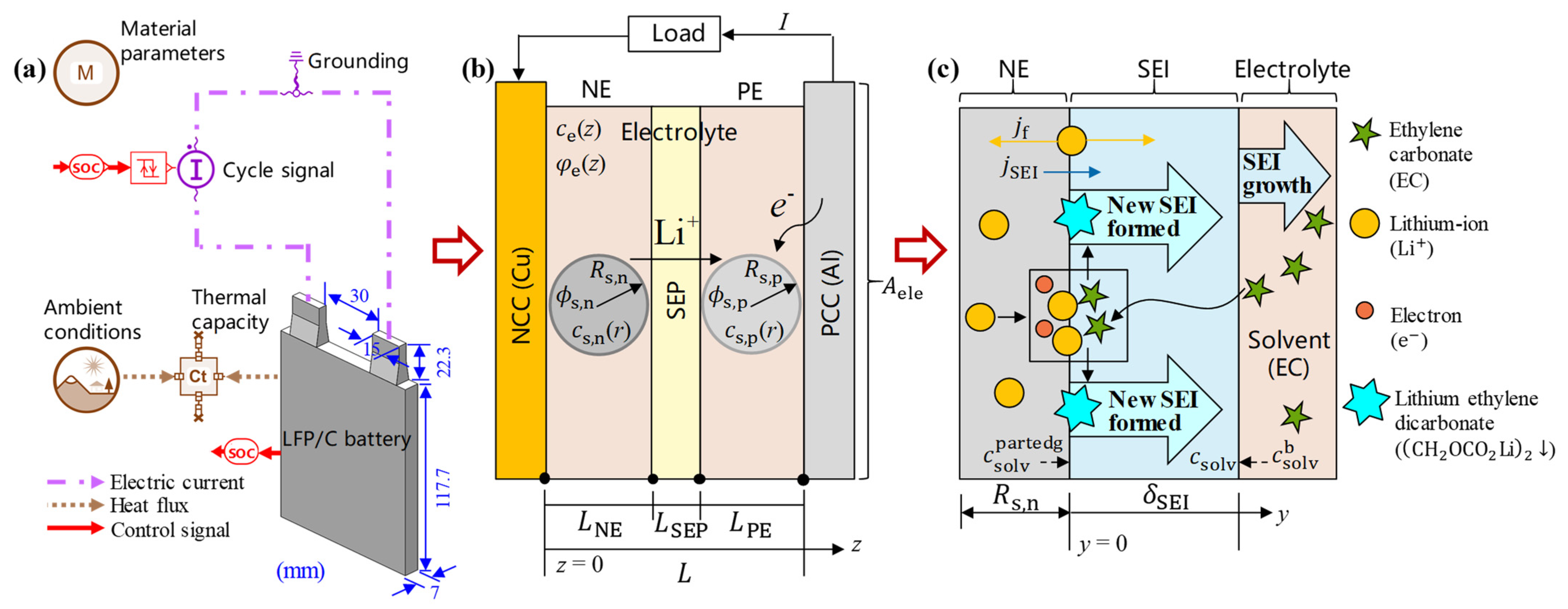
2.1. Charge–Discharge and Nominal Electrochemical Model of the Battery Cell

The characteristics and the geometry of the LFP battery have been discussed in our previous work [29] and are listed in

Table 1. The technical specifications and thermophysical parameters of the battery cell.

Parameter	Value
Cell length	140 mm
Cell width	70 mm
Cell thickness	7 mm
Nominal voltage	3.2 V
Charge cut-off voltage	3.65 V
Discharge cut-off voltage	2 V
Nominal capacity	5 $\mathrm{A}·\mathrm{h}$
Energy density	245 $\mathrm{Wh}·{\mathrm{L}}^{-1}$
Positive electrode material	LiFePO4
Negative electrode material	Graphite-based carbon
Electrolyte material	Carbonate based
Thermal conductivity, $k_{\mathrm{b}}$ ($\mathrm{W}·{\mathrm{m}}^{-1}·{\mathrm{K}}^{-1}$)	55.66
Density, ${\rho }_{\mathrm{b}}$ ($\mathrm{kg}·{\mathrm{m}}^{-3}$)	2318.07
Specific thermal capacity, $C_{\mathrm{p},\mathrm{b}}$ ($\mathrm{J}·{\mathrm{kg}}^{-1}·{\mathrm{K}}^{-1}$)	1056.08

. The electrochemical reactions can be expressed as in [46].

The reaction at the positive electrode is:

$${\mathrm{Li}}_{1-i}\mathrm{FeP}{\mathrm{O}}_4+i{\mathrm{Li}}^{+}+i{\mathrm{e}}^{-}\underset{\mathrm{charge}}{\overset{\mathrm{discharge}}{\rightleftharpoons }}\mathrm{Li}\mathrm{FeP}{\mathrm{O}}_4$$

(1)

The reaction at the negative electrode is:

$${\mathrm{Li}}_j{\mathrm{C}}_6{\displaystyle \underset{\mathrm{charge}}{\overset{\mathrm{discharge}}{\rightleftharpoons }}}{\mathrm{Li}}_{1-j}{\mathrm{C}}_6+j{\mathrm{Li}}^{+}+j{\mathrm{e}}^{-}$$

(2)

Figure 1a shows the charge–discharge model of the battery, including the battery model, thermal boundary condition, electrical connection, and cycle signal of the charge–discharge process. The thermophysical parameters are described by the material parameters module (listed in Table 1) and the part of the battery in contact with the air is described by the ambient conditions module, as shown in Figure 1a. The equation can be expressed as:

$$Q_{\mathrm{tra}}=h_{\mathrm{conv}}{A}_{\mathrm{b}}\left(T_{\mathrm{b}}-T_{\mathrm{amb}}\right)+{\sigma }_{\mathrm{B}}\chi \left(T_{\mathrm{b}}^4-T_{\mathrm{amb}}^4\right)$$

(3)

where $Q_{\mathrm{tra}}$ is the heat transferred from the battery to the ambient air. $h_{\mathrm{conv}}$ is the convective heat transfer coefficient and $\chi$ is the surface emissivity, and they are set as 10 $\mathrm{W}·{\mathrm{m}}^{-2}·{\mathrm{K}}^{-1}$ [32] and 0.8 [47], respectively. $A_{\mathrm{b}}$ is the area between the battery and the ambient air. ${\sigma }_{\mathrm{B}}$ is the Stefan–Boltzmann constant. $T_{\mathrm{b}}$ and $T_{\mathrm{amb}}$ are the battery temperature and ambient temperature, respectively. The electrochemical model chosen is a simplification of the pseudo-two-dimensional model (proposed by Doyle–Fuller–Newman [37] and described in detail in our previous work [48]) called the single particle (SP) model where the solid phase is modeled as a single particle, as shown in Figure 1b. This model has been widely used in the one-dimensional simulation software, AMESim (Advanced Modeling Environment for performing Simulation of engineering systems). The thickness direction contains five parts: a negative current collector (NCC), a negative electrode (NE), a separator (SEP), a positive electrode (PE), and a positive current collector (PCC), as shown in Figure 1b. In the SP model, the electrode is regarded as the superposition of two continuums, namely the electrolytic phase and a solid matrix, as shown in Figure 1b. The models of solid matrices are microscopic spherical particles in which Li-ions diffuse and react on the surface of the spheres. The main hypotheses [49] of this model are:

(1)

The passive sign convention is used: $I>0$ during charge and $I<0$ during discharge;

(2)

The particles in both electrodes can be represented as two mean spherical particles;

(3)

The active surface is assumed to be same in all areas: $S_{\mathrm{p}}=S_{\mathrm{sep}}=S_{\mathrm{n}}=A_{\mathrm{ele}}$.

The SP model computes the battery voltage based on its internal state and external solicitations. The voltage is the difference between the potential of its electrodes summed with the electrolyte potential [50]:

$$U\left(t\right)={\varphi }_{\mathrm{s}}\left(L\right)-{\varphi }_{\mathrm{s}}\left(0\right)=U_{\mathrm{p}}-U_{\mathrm{n}}+\eta \left(L\right)-\eta \left(0\right)+{\varphi }_{\mathrm{e}}\left(L\right)-{\varphi }_{\mathrm{e}}\left(0\right),$$

(4)

where $U_{\mathrm{p}}$ and $U_{\mathrm{n}}$ are the thermodynamic potential of the PE and NE, respectively.$\eta \left(L\right)$ and $\eta \left(0\right)$ are the overpotentials at z = L and z = 0, respectively. z is the battery thickness direction, as shown in Figure 1b. ${\varphi }_{\mathrm{e}}\left(L\right)$ and ${\varphi }_{\mathrm{e}}\left(0\right)$ are the electrolyte potentials at z = L and z = 0, respectively. Thermodynamic potentials are evaluated from the solid concentration of Li in the bulk (R = 0) of the single particle:

$$U_{\mathrm{p}}=U_{\mathrm{p}}^{\mathrm{ref}}\left(x_{\mathrm{p}}\right)=U_{\mathrm{p}}^{\mathrm{ref}}\left(\frac{c_{\mathrm{s},\mathrm{p}}^{\mathrm{b}}}{c_{\mathrm{s},\mathrm{p}}^{\max }}\right), U_{\mathrm{n}}=U_{\mathrm{n}}^{\mathrm{ref}}\left(x_{\mathrm{n}}\right)=U_{\mathrm{n}}^{\mathrm{ref}}\left(\frac{c_{\mathrm{s},\mathrm{n}}^{\mathrm{b}}}{c_{\mathrm{s},\mathrm{n}}^{\max }}\right),$$

(5)

where $\frac{c_{\mathrm{s},\mathrm{p}}^{\mathrm{b}}}{c_{\mathrm{s},\mathrm{p}}^{\max }}$ and $\frac{c_{\mathrm{s},\mathrm{n}}^{\mathrm{b}}}{c_{\mathrm{s},\mathrm{n}}^{\max }}$ correspond to the coefficients i and j used in Equations (1) and (2), respectively. $c_{\mathrm{s},\mathrm{p}}^{\mathrm{b}}$ and $c_{\mathrm{s},\mathrm{n}}^{\mathrm{b}}$ are the bulk Li concentrations in the solid phase for PE and NE, respectively. $c_{\mathrm{s},\mathrm{p}}^{\max }$ and $c_{\mathrm{s},\mathrm{n}}^{\max }$ are the maximum Li concentrations in the PE and NE, respectively. $U_{\mathrm{p}}^{\mathrm{ref}}$ and $U_{\mathrm{n}}^{\mathrm{ref}}$ are the reference potentials of the PE and NE, respectively. The nominal physical and chemical phenomena occurring in Li-ion systems can be expressed by the mass conservation of Li⁺ species, charge conservation, and electrochemical kinetics, as shown in

Table 2. Equations in the electrochemical model.

Physical and Chemical Mechanisms	Equations	Boundary Conditions
Solid phase: conservation of Li+ species	$\frac{\partial }{\partial t}{c}_{\mathrm{s}}-\frac{1}{r^2}\frac{\partial }{\partial r}\left(r^2{D}_{\mathrm{s}}\frac{\partial }{\partial r}{c}_{\mathrm{s}}\right)=0$	${D_{\mathrm{s}}\frac{\partial }{\partial r}{c}_{\mathrm{s}}|}_{r=0}=0, {-D_{\mathrm{s}}\frac{\partial }{\partial r}{c}_{\mathrm{s}}|}_{r=R_{\mathrm{s}}}=\frac{j_{\mathrm{f}}}{a_{\mathrm{s}}F}$
Electrolyte phase: conservation of Li+ species	$\frac{\partial }{\partial t}{\epsilon }_{\mathrm{e}}{c}_{\mathrm{e}}-\frac{\partial }{\partial z}\left(D_{\mathrm{e}}^{\mathrm{eff}}\frac{\partial }{\partial z}{c}_{\mathrm{e}}\right)-\left(1-t_{+}\right)\frac{j_{\mathrm{f}}}{F}=0$	${\frac{\partial }{\partial z}{c}_{\mathrm{e}}|}_{z=0}={\frac{\partial }{\partial z}{c}_{\mathrm{e}}|}_{z=L}=0$
Solid phase: charge conservation	$\frac{\partial }{\partial z}\left({\sigma }^{\mathrm{eff}}\frac{\partial }{\partial z}{\varphi }_{\mathrm{s}}\right)-j_{\mathrm{f}}=0$	${-{\sigma }_{\mathrm{e}}^{\mathrm{eff}}\frac{\partial }{\partial z}{\varphi }_{\mathrm{s}}|}_{z=0}={-{\sigma }^{\mathrm{eff}}\frac{\partial }{\partial z}{\varphi }_{\mathrm{s}}|}_{z=L}=\frac{I}{A_{\mathrm{ele}}},$ ${\frac{\partial }{\partial z}{\varphi }_{\mathrm{s}}|}_{z=L_{\mathrm{NE}}}={\frac{\partial }{\partial z}{\varphi }_{\mathrm{s}}|}_{z=L-L_{\mathrm{PE}}}=0$
Electrolyte phase: charge conservation	$\frac{\partial }{\partial z}\left({\kappa }^{\mathrm{eff}}\frac{\partial }{\partial z}{\varphi }_{\mathrm{e}}\right)+\frac{\partial }{\partial z}\left({\kappa }_D^{\mathrm{eff}}\frac{\partial }{\partial z}\ln c_{\mathrm{e}}\right)+j_{\mathrm{f}}=0$	${\frac{\partial }{\partial z}{\varphi }_{\mathrm{e}}|}_{z=0}={\frac{\partial }{\partial z}{\varphi }_{\mathrm{e}}|}_{z=L}=0$
Electrochemical kinetics	$j_{\mathrm{f}}=a_{\mathrm{s}}{i}_0\left[\exp \left(\frac{{\alpha }_{\mathrm{ox}}F}{RT}\eta \right)-\exp \left(\frac{-{\alpha }_{\mathrm{red}}F}{RT}\eta \right)\right]$
Electrolyte ionic diffusivity	$D_{\mathrm{e}}^{\mathrm{eff}}$=$D_{\mathrm{e}}{\epsilon }_{\mathrm{e}}^{{\gamma }_{\mathrm{e}}}$
Electrolyte ionic conductivity	${\kappa }^{\mathrm{eff}}=\kappa {\epsilon }_{\mathrm{e}}^{{\gamma }_{\mathrm{e}}}$
Electrolyte ionic diffusional conductivity	${\kappa }_D^{\mathrm{eff}}=\frac{2RT}{F}{\kappa }^{\mathrm{eff}}\left(t_{+}-1\right)\left(1+\frac{d\ln f_{\pm }}{d\ln c_{\mathrm{e}}}\right)$
Solid phase electronic conductivity	${\sigma }^{\mathrm{eff}}=\sigma {\epsilon }_{\mathrm{s}}{}^{{\gamma }_{\mathrm{s}}}$
Specific interfacial surface area	$a_{\mathrm{s}}=\frac{3{\epsilon }_{\mathrm{s}}}{R_{\mathrm{s}}}$

. All these equations are coupled into the framework of the P2D electrochemical model and have been discussed in previous works [45,48].

The diffusion of the solid phase leads to solid phase overpotential, which can be approximated as the difference between the bulk thermodynamic potential and the thermodynamic potential at the surface of the particles [50]:

$$U_{\mathrm{p}}=U_{\mathrm{p}}^{\mathrm{ref}}\left(x_{\mathrm{p}}\right)=U_{\mathrm{p}}^{\mathrm{ref}}\left(\frac{c_{\mathrm{s},\mathrm{p}}^{\mathrm{b}}}{c_{\mathrm{s},\mathrm{p}}^{\max }}\right), U_{\mathrm{n}}=U_{\mathrm{n}}^{\mathrm{ref}}\left(x_{\mathrm{n}}\right)=U_{\mathrm{n}}^{\mathrm{ref}}\left(\frac{c_{\mathrm{s},\mathrm{n}}^{\mathrm{b}}}{c_{\mathrm{s},\mathrm{n}}^{\max }}\right),$$

(6)

where $c_{\mathrm{s},\mathrm{p}}^{R_{\mathrm{s},\mathrm{p}}}$ and $c_{\mathrm{s},\mathrm{n}}^{R_{\mathrm{s},\mathrm{n}}}$ are the Li concentrations at the solid–electrolyte interface phase, where the subscripts p and n denote PE and NE, respectively. The solid ohmic overpotentials can be calculated as [50]:

$$U_{\mathrm{p}}=U_{\mathrm{p}}^{\mathrm{ref}}\left(x_{\mathrm{p}}\right)=U_{\mathrm{p}}^{\mathrm{ref}}\left(\frac{c_{\mathrm{s},\mathrm{p}}^{\mathrm{b}}}{c_{\mathrm{s},\mathrm{p}}^{\max }}\right), U_{\mathrm{n}}=U_{\mathrm{n}}^{\mathrm{ref}}\left(x_{\mathrm{n}}\right)=U_{\mathrm{n}}^{\mathrm{ref}}\left(\frac{c_{\mathrm{s},\mathrm{n}}^{\mathrm{b}}}{c_{\mathrm{s},\mathrm{n}}^{\max }}\right),$$

(7)

where ${\sigma }_{\mathrm{p}}^{\mathrm{eff}}$ and ${\sigma }_{\mathrm{n}}^{\mathrm{eff}}$ are the effective solid phase conductivities of the PE and NE, respectively. $L_{\mathrm{PE}}$ and $L_{\mathrm{NE}}$ are the thicknesses of the PE and NE, respectively. $I$ is the electric current and $A_{\mathrm{ele}}$ is the geometric area of the electrodes. The electrolyte diffusion overpotential due to the Li concentration gradient in the electrolyte can be calculated as [50]:

$${\eta }_{\mathrm{e}}^{\mathrm{diff}}=\left(1-t_{+}\right)2\frac{RT}{F}\ln \frac{c_{\mathrm{e}}\left(L\right)}{c_{\mathrm{e}}\left(0\right)},$$

(8)

where $t_{+}$ is the Li transference number.$c_{\mathrm{e}}\left(L\right)$ and $c_{\mathrm{e}}\left(0\right)$ are the Li concentrations in the electrolyte phase at z = L and z = 0, respectively. $R$ is the ideal gas constant, $T$ is the temperature, and $F$ is the Faraday constant. The electrolyte ohmic overpotential due to electrolyte conductivity can be calculated as [50]:

$${\eta }_{\mathrm{e}}^{\mathrm{ohm}}=\frac{I}{2A_{\mathrm{ele}}}\left(\frac{L_{\mathrm{NE}}}{{\kappa }_{\mathrm{n}}^{\mathrm{eff}}}+\frac{2L_{\mathrm{SEP}}}{{\kappa }_{\mathrm{SEP}}^{\mathrm{eff}}}+\frac{L_{\mathrm{PE}}}{{\kappa }_{\mathrm{p}}^{\mathrm{eff}}}\right),$$

(9)

where ${\kappa }_{\mathrm{n}}^{\mathrm{eff}}$, ${\kappa }_{\mathrm{SEP}}^{\mathrm{eff}}$, and ${\kappa }_{\mathrm{p}}^{\mathrm{eff}}$ are the electrolyte effective ionic conductivities in the NE, SEP, and PE, respectively. $L_{\mathrm{SEP}}$ is the thickness of SEP. The oxidation and reduction charge transfer coefficients, ${\alpha }_{\mathrm{ox}}$ and ${\alpha }_{\mathrm{red}}$, are assumed to be equal to 0.5 for both electrodes. The positive and negative kinetic overpotentials can be expressed as [50]:

$${\eta }_{\mathrm{p}}^{\mathrm{k}}=2\frac{RT}{F}\ln \left({\xi }_{\mathrm{p}}+\sqrt{{\xi }_{\mathrm{p}}^2+1}\right),{\eta }_{\mathrm{n}}^{\mathrm{k}}=2\frac{RT}{F}\ln \left({\xi }_{\mathrm{n}}+\sqrt{{\xi }_{\mathrm{n}}^2+1}\right),$$

(10)

where

$${\xi }_{\mathrm{p}}=\frac{I}{2i_{0,\mathrm{p}}{S}_{\mathrm{p}}}=\frac{R_{\mathrm{s},\mathrm{p}}}{6{\epsilon }_{\mathrm{s},\mathrm{p}}{i}_{0,\mathrm{p}}{A}_{\mathrm{ele}}{L}_{\mathrm{PE}}}I, {\xi }_{\mathrm{n}}=\frac{I}{2i_{0,\mathrm{p}}{S}_{\mathrm{n}}}=\frac{R_{\mathrm{s},\mathrm{n}}}{6{\epsilon }_{\mathrm{s},\mathrm{n}}{i}_{0,\mathrm{n}}{A}_{\mathrm{ele}}{L}_{\mathrm{NE}}}I,$$

(11)

where $S_{\mathrm{p}}$ and $S_{\mathrm{n}}$ are the area of PE and NE, respectively. $R_{\mathrm{s},\mathrm{p}}$ and $R_{\mathrm{s},\mathrm{n}}$ are the particle radii in the PE and NE, respectively. ${\epsilon }_{\mathrm{s},\mathrm{p}}$ and ${\epsilon }_{\mathrm{s},\mathrm{n}}$ are the volume fractions of the active material in the PE and NE, respectively. The exchange current densities can be expressed as [50]:

$$\begin{gathered} i_{0,\mathrm{p}}=k_{0,\mathrm{p}}F{\left(c_{\mathrm{e}}\right)}^{{\alpha }_{\mathrm{ox},\mathrm{p}}}{\left(c_{\mathrm{s},\mathrm{p}}^{R_{\mathrm{s},\mathrm{p}}}\right)}^{{\alpha }_{\mathrm{ox},\mathrm{p}}}{\left(c_{\mathrm{s},\mathrm{p}}^{\max }-c_{\mathrm{s},\mathrm{p}}^{R_{\mathrm{s},\mathrm{p}}}\right)}^{{\alpha }_{\mathrm{ox},\mathrm{p}}} \\ {i}_{0,\mathrm{n}}=k_{0,\mathrm{n}}F{\left(c_{\mathrm{e}}\right)}^{{\alpha }_{\mathrm{ox},\mathrm{n}}}{\left(c_{\mathrm{s},\mathrm{n}}^{R_{\mathrm{s},\mathrm{n}}}\right)}^{{\alpha }_{\mathrm{ox},\mathrm{n}}}{\left(c_{\mathrm{s},\mathrm{n}}^{\max }-c_{\mathrm{s},\mathrm{n}}^{R_{\mathrm{s},\mathrm{n}}}\right)}^{{\alpha }_{\mathrm{ox},\mathrm{n}}}, \end{gathered}$$

(12)

where $c_{\mathrm{e}}$ is the Li-ion concentration in the electrolyte phase and ${\alpha }_{\mathrm{ox},\mathrm{p}}$ and ${\alpha }_{\mathrm{ox},\mathrm{n}}$ represent the oxidation charge transfer coefficients of the PE and NE, respectively.$k_{0,\mathrm{p}}$ and $k_{0,\mathrm{n}}$ are the reaction rate constants of the PE and NE, respectively. By combining these equations, the output voltage (Equation (4)) of the battery can be expressed as:

$$U\left(t\right)=U_{\mathrm{p}}^{\mathrm{ref}}\left(\frac{c_{\mathrm{s},\mathrm{p}}^{R_{\mathrm{s},\mathrm{p}}}}{c_{\mathrm{s},\mathrm{p}}^{\max }}\right)-U_{\mathrm{n}}^{\mathrm{ref}}\left(\frac{c_{\mathrm{s},\mathrm{n}}^{R_{\mathrm{s},\mathrm{n}}}}{c_{\mathrm{s},\mathrm{n}}^{\max }}\right)+{\eta }_{\mathrm{s},\mathrm{p}}^{\mathrm{ohm}}-{\eta }_{\mathrm{s},\mathrm{n}}^{\mathrm{ohm}}+{\eta }_{\mathrm{e}}^{\mathrm{ohm}}+{\eta }_{\mathrm{e}}^{\mathrm{diff}}+{\eta }_{\mathrm{p}}^{\mathrm{k}}-{\eta }_{\mathrm{n}}^{\mathrm{k}}$$

(13)

It is important to note that Equation (13) does not take into account the battery aging. The expression of battery voltage considering the battery aging is shown in Equation (20).

2.2. Aging Model of the Battery Cell

Battery aging results in capacity and power losses due to several physical mechanisms. The physical mechanism taken into account in this study is the formation of a solid electrolyte interface (SEI) layer on the NE. In addition, its effects on the battery behavior are considered. SEI layer formation is a phenomenon occurring on a negative carbonaceous electrode when its potential is low [49]. Under these conditions, Li starts a reaction with the solvent of the electrolyte which forms the SEI, as shown in Figure 1c. The reaction equation is [51]:

$$2\mathrm{EC}+2{\mathrm{e}}^{-}+2{\mathrm{Li}}^{+}\Rightarrow {\left({\mathrm{CH}}_2{\mathrm{OCO}}_2\mathrm{Li}\right)}_2\downarrow +{\mathrm{C}}_2{\mathrm{H}}_4\uparrow$$

(14)

During this reaction, lithium is withdrawn from the NE and trapped in the SEI. This leads to a loss of cycling Li and thus a capacity loss. In addition, the SEI formed is a resistive layer leading to an increase in the resistance. As described in Figure 1c, the electrolyte solvent is transported from the electrolyte bulk to the particle surface of the SEI, it then reacts and forms a new SEI. Equations involved in the aging calculation have been comprehensively discussed in previous work [48] and are listed here in

Table 3. Equations solved for the aging model.

Physical and Chemical Mechanisms	Equations	Boundary Conditions
SEI formation reaction kinetics	$j_{\mathrm{SEI}}=2F{k}_{\mathrm{SEI}}{c}_{\mathrm{solv}}^{\mathrm{partedg}}{c}_{\mathrm{s},\mathrm{n}}{\left(r=R_{\mathrm{s},\mathrm{n}}\right)}^2$ $\exp \left(-\frac{{\beta }_{\mathrm{SEI}}F}{RT}·\left(\frac{-{\delta }_{\mathrm{SEI}}I}{{\kappa }_{\mathrm{SEI}}{S}_{\mathrm{n}}}\right)\right)$ $\exp \left(-\frac{{\beta }_{\mathrm{SEI}}F}{RT}\left({\varphi }_{\mathrm{s},\mathrm{n}}-U_{\mathrm{SEI}}\right)\right)$
Solvent diffusion in the SEI	$\frac{\partial c_{\mathrm{solv}}}{\partial t}=D_{\mathrm{solv}}\frac{{\partial }^2{c}_{\mathrm{solv}}}{\partial y^2}-\frac{d{\delta }_{\mathrm{SEI}}}{dt}\frac{\partial c_{\mathrm{solv}}}{\partial y}$	$D_{\mathrm{solv}}{\frac{\partial c_{\mathrm{solv}}}{\partial y}|}_{y=R_{\mathrm{s},\mathrm{n}}}-\frac{d{\delta }_{\mathrm{SEI}}}{dt}{c}_{\mathrm{solv}}^{\mathrm{partedg}}=-\frac{j_{\mathrm{SEI}}}{2F},$ $c_{\mathrm{solv}}\left(r=R_{\mathrm{s},\mathrm{n}}+{\delta }_{\mathrm{SEI}}\right)={\epsilon }_{\mathrm{SEI}}{c}_{\mathrm{solv}}^{\mathrm{b}}$
Loss of capacity variation	$\frac{d{C}_{\mathrm{loss}}^{\mathrm{SEI}}}{dt}=\frac{j_{\mathrm{SEI}}{S}_{\mathrm{n}}}{3600}$ ${\mathrm{LOC}}_{\mathrm{SEI}}=\frac{C_{\mathrm{loss}}^{\mathrm{SEI}}}{C_{\mathrm{tot}}}\times 100$
SEI porosity variation	$\frac{d{\epsilon }_{\mathrm{SEI}}}{dt}=\frac{-j_{\mathrm{SEI}}{S}_{\mathrm{n}}}{3600C_{\mathrm{loss}}^{\mathrm{SEI}}}\left(1-{\epsilon }_{\mathrm{SEI}}\right)\left(1-\frac{1-{\epsilon }_{\mathrm{SEI}}}{1-{\epsilon }_{\mathrm{SEI}}^{*}}\right)$
SEI layer thickness	${\delta }_{\mathrm{SEI}}=\frac{3600C_{\mathrm{loss}}^{\mathrm{SEI}}{M}_{\mathrm{SEI}}}{2F{\rho }_{\mathrm{SEI}}{S}_{\mathrm{n}}\left(1-{\epsilon }_{\mathrm{SEI}}\right)}$

.

It is worth mentioning that ${\epsilon }_{\mathrm{SEI}}^{*}$ is the instantaneously formed SEI layer porosity. ${\epsilon }_{\mathrm{SEI}}$ is the SEI layer porosity. The ohmic overvoltage can be calculated as [52]:

$${\eta }_{\mathrm{SEI}}=-\frac{{\delta }_{\mathrm{SEI}}}{{\kappa }_{\mathrm{SEI}}{S}_{\mathrm{n}}}I, {\kappa }_{\mathrm{SEI}}={\kappa }_{\mathrm{SEI},\mathrm{data}}{\left(1-{\epsilon }_{\mathrm{SEI}}\right)}^{{\gamma }_{\mathrm{SEI}}},$$

(15)

where ${\kappa }_{\mathrm{SEI},\mathrm{data}}$ is the index of the SEI layer electronic conductivity data and ${\gamma }_{\mathrm{SEI}}$ is the SEI Bruggeman exponent. $c_{\mathrm{solv}}$ is the concentration of the solvent inside the SEI layer. The bulk solvent concentration, $c_{\mathrm{solv}}^{\mathrm{b}}$, is considered to be constant outside the SEI layer, as shown in Figure 1c. Based on these equations, it is possible to evaluate the solvent concentration, $c_{\mathrm{solv}}$, and then the parasitic current of the SEI formation, $j_{\mathrm{SEI}}$, can be calculated. Furthermore, the variation in the SEI porosity, capacity loss, and the SEI layer thickness can be calculated.

For dynamic aging modeling, when the model is initialized, previous aging needs to be taken into account. Firstly, based on the initial capacity loss, the initial insertion rate of the NE can be modified as:

$$x_{\mathrm{n},\mathrm{int}}=x_{\mathrm{n},0}+\frac{3600\frac{{\mathrm{SOC}}_{\mathrm{int}}}{100}\left(C_{\mathrm{nom}}-C_{\mathrm{loss},\mathrm{int}}^{\mathrm{SEI}}\right)}{A_{\mathrm{ele}}{L}_{\mathrm{NE}}{\epsilon }_{\mathrm{s},\mathrm{n}}F{c}_{\mathrm{s},\mathrm{n}}^{\max }},$$

(16)

where $x_{\mathrm{n},0}$ is the negative insertion rate when the state of charge is zero (SOC = 0), ${\mathrm{SOC}}_{\mathrm{int}}$ is the initial SOC, $C_{\mathrm{nom}}$ is the nominal capacity, and $C_{\mathrm{loss},\mathrm{int}}^{\mathrm{SEI}}$ is the initial cycling Li loss due to SEI formation. Secondly, using the bulk solvent concentration and the battery average temperature, the initial solvent concentrations in the SEI layers can be calculated. With the assumption of a stationary state, it is assumed that the input current is 0 A and all time derivatives are null.

$$\frac{d{\epsilon }_{\mathrm{SEI}}}{dt}=0, \frac{\partial c_{\mathrm{solv}}}{\partial t}=0$$

(17)

There are several different consequences of aging on cell behavior. First, the current resulting from the parasitic reaction needs to be taken into account in the solid phase Li conservation. Therefore, the boundary condition of solid-phase Li⁺ conservation in Table 2 can be modified as:

$${-D_{\mathrm{s}}\frac{\partial c_{\mathrm{s},\mathrm{n}}}{\partial r}|}_{r=R_{\mathrm{s}}}=\frac{j_{\mathrm{f}}}{a_{\mathrm{s}}F}+\frac{j_{\mathrm{SEI}}}{F}$$

(18)

Then, the porosity of the NE is modified due to the clogging of pores by the SEI layer [52]:

$${\epsilon }_{\mathrm{e},\mathrm{n}}={\epsilon }_{\mathrm{e},\mathrm{n},\mathrm{int}}-{\epsilon }_{\mathrm{s},\mathrm{n}}\frac{3{\delta }_{\mathrm{SEI}}\left(t\right)}{R_{\mathrm{s},\mathrm{n}}},$$

(19)

where ${\epsilon }_{\mathrm{e},\mathrm{n},\mathrm{int}}$ is the initial porosity of the NE. In the event of a SEI layer that is too thick, the porosity is completely clogged. At this point, the battery reaches the end of its life and the model stops. The final effect is the increase in resistance due to the growth of the SEI layer. Another ohmic drop is added to the final voltage to take into account the effect of the SEI on the cell voltage; therefore, Equation (13) can be modified as:

$$U\left(t\right)=U_{\mathrm{p}}^{\mathrm{ref}}\left(\frac{c_{\mathrm{s},\mathrm{p}}^{R_{\mathrm{s},\mathrm{p}}}}{c_{\mathrm{s},\mathrm{p}}^{\max }}\right)-U_{\mathrm{n}}^{\mathrm{ref}}\left(\frac{c_{\mathrm{s},\mathrm{n}}^{R_{\mathrm{s},\mathrm{n}}}}{c_{\mathrm{s},\mathrm{n}}^{\max }}\right)+{\eta }_{\mathrm{s},\mathrm{p}}^{\mathrm{ohm}}-{\eta }_{\mathrm{s},\mathrm{n}}^{\mathrm{ohm}}+{\eta }_{\mathrm{e}}^{\mathrm{ohm}}+{\eta }_{\mathrm{e}}^{\mathrm{diff}}+{\eta }_{\mathrm{p}}^{\mathrm{k}}-{\eta }_{\mathrm{n}}^{\mathrm{k}}-{\eta }_{\mathrm{SEI}}$$

(20)

The total current intensity in the NE can be expressed as:

$$j_{\mathrm{tot}}=j_{\mathrm{f}}+a_{\mathrm{s},\mathrm{n}}{j}_{\mathrm{SEI}}$$

(21)

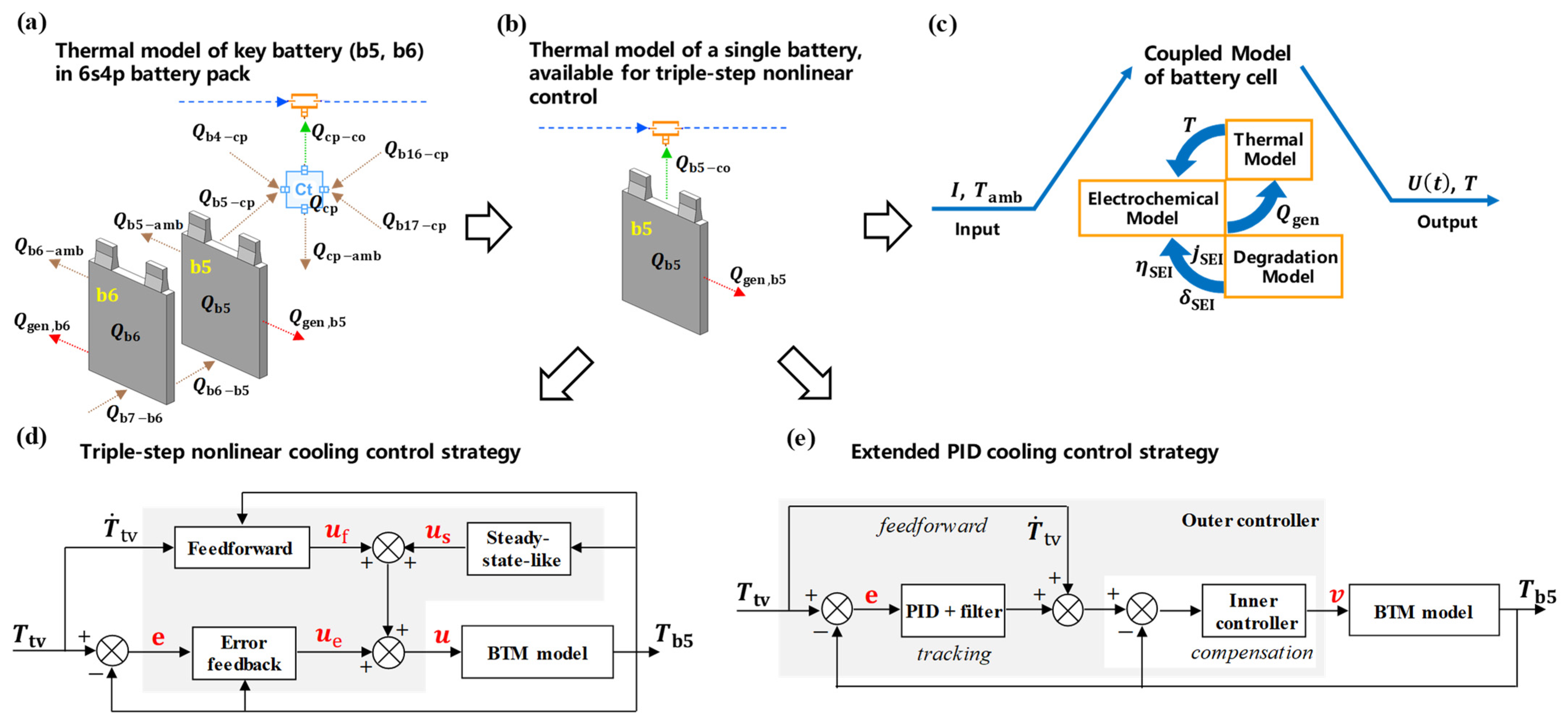
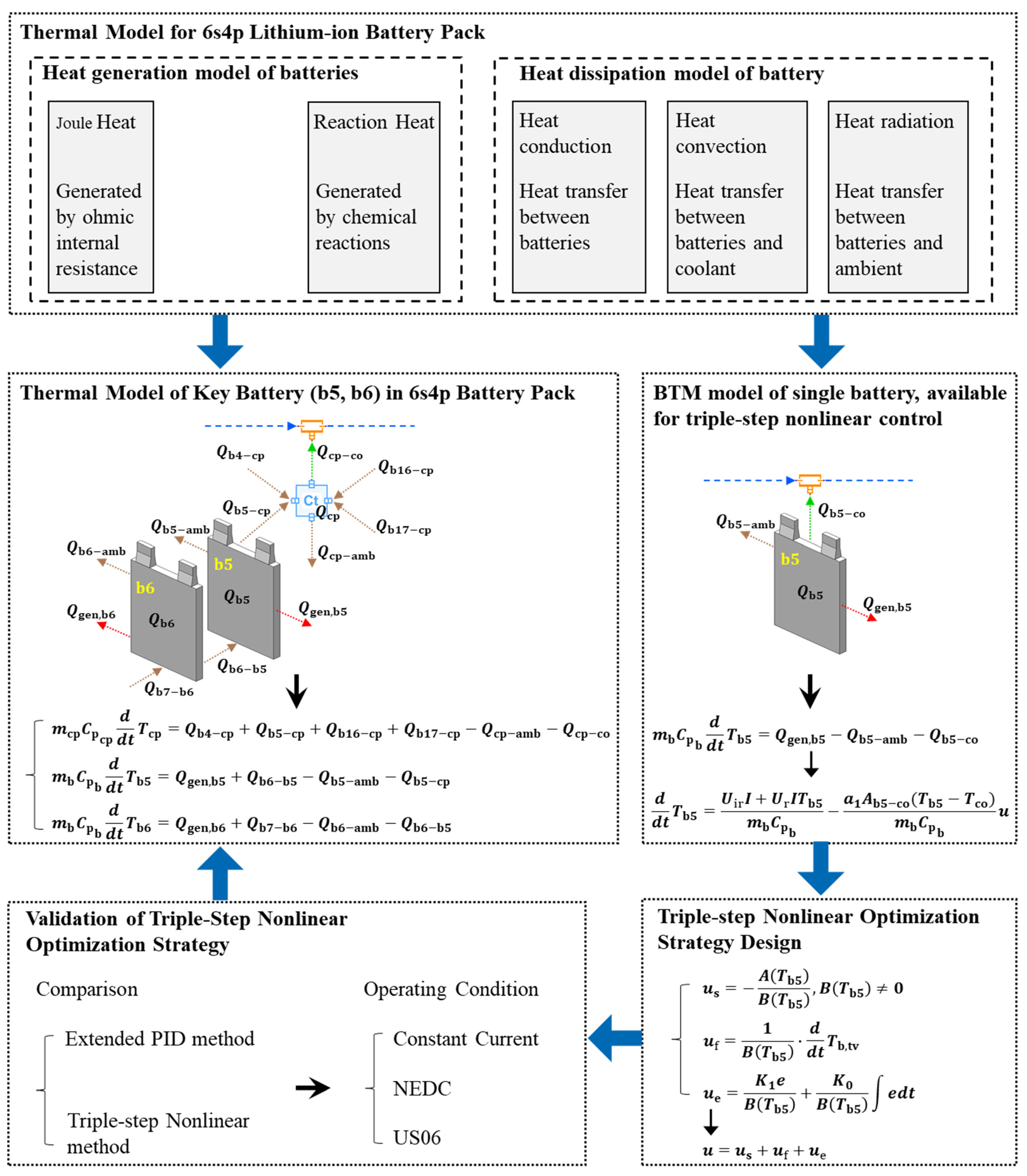
2.3. Thermal Models of the Battery Cell

The generated heat is described classically as the sum of irreversible and reversible heats [52]:

$$Q_{\mathrm{gen}}=-\left(\left({\eta }_{\mathrm{s},\mathrm{p}}^{\mathrm{ohm}}-{\eta }_{\mathrm{s},\mathrm{n}}^{\mathrm{ohm}}+{\eta }_{\mathrm{e}}^{\mathrm{ohm}}+{\eta }_{\mathrm{e}}^{\mathrm{diff}}+{\eta }_{\mathrm{p}}^{\mathrm{k}}-{\eta }_{\mathrm{n}}^{\mathrm{k}}-{\eta }_{\mathrm{SEI}}\right)I+T\left(\frac{d{U}_{\mathrm{p}}}{dT}\left(x_{\mathrm{p}}\right)-\frac{d{U}_{\mathrm{n}}}{dT}\left(x_{\mathrm{n}}\right)\right)I\right),$$

(22)

the first and second items on the right are the Joule effect and entropic effect in the battery, respectively. The equation of convective and radiative heat transfer is shown in Equation (3). Therefore, the energy balance of the battery cell can be expressed as:

$$\frac{d}{dt}T=\frac{1}{m_{\mathrm{b}}{C}_{\mathrm{p}}{}_{\mathrm{b}}}\left(Q_{\mathrm{gen}}-Q_{\mathrm{tra}}\right),$$

(23)

where $m_{\mathrm{b}}$ and $C_{\mathrm{p}}{}_{\mathrm{b}}$ are the mass and specific thermal capacity of the battery cell, respectively. The nominal electrochemical model, thermal model, and aging model are coupled to study the battery performance. Several parameters are temperature dependent, and the Arrhenius law [52,53,54] can be used to evaluate these parameters, as shown in

Table 4. Equations for the temperature-dependent parameters.

Parameters	Equations	Refs.
Active material in solid phase
Solid phase diffusivity $\left(D_{\mathrm{s}}\right)$	$D_{\mathrm{s},\mathrm{p}}=5.9\times {10}^{-20}\exp \left(-\frac{\mathrm{50,000}}{8.314}\left(\frac{1}{T}-\frac{1}{298}\right)\right)$	[50,52]
	$D_{\mathrm{s},\mathrm{n}}=3\times {10}^{-15}\exp \left(-\frac{\mathrm{35,000}}{8.314}\left(\frac{1}{T}-\frac{1}{298}\right)\right)$	[50,52]
Solid phase conductivity ($\sigma$)	${\sigma }_{\mathrm{p}}=0.7\exp \left(-\frac{\mathrm{10,000}}{8.314}\left(\frac{1}{T}-\frac{1}{298}\right)\right)$	[50,52]
	${\sigma }_{\mathrm{n}}=100\exp \left(-\frac{\mathrm{11,000}}{8.314}\left(\frac{1}{T}-\frac{1}{298}\right)\right)$	[50,52]
Electrode reaction rate constant ($k_0$)		[50,52]
	$k_{0,\mathrm{n}}=1.5\times {10}^{-10}\exp \left(-\frac{\mathrm{20,000}}{8.314}\left(\frac{1}{T}-\frac{1}{298}\right)\right)$	[50,52]
Electrolyte
Electrolyte ionic diffusivity ($D_{\mathrm{e}}$)	$D_{\mathrm{e}}=1\times {10}^{-4}\times {10}^{-4.43-\frac{54}{T-229}}\exp \left(-\frac{c_{\mathrm{e}}}{-0.26795T^2+169.99T-\mathrm{25,342}}\right)$	[50,52]
Electrolyte ionic conductivity ($\kappa$)	$\kappa =\left(-1.5069\times {10}^{-2}+8.8078\times {10}^{-5}T-9.4814\times {10}^{-8}{T}^2\right)c_{\mathrm{e}}\exp \left(\left(-1.5799\times {10}^{-3}+7.8183\times {10}^{-6}T-1.0513\times {10}^{-8}{T}^2\right)c_{\mathrm{e}}{}^{1.2167}\right)$	[50,52]
SEI formation
SEI formation reaction rate constant ($k_{\mathrm{SEI}}$)	$k_{\mathrm{SEI}}=2.9465\times {10}^{-26}\exp \left(-\frac{\mathrm{149,150}}{8.314}\left(\frac{1}{T}-\frac{1}{298}\right)\right)$	[50,52]
SEI solvent diffusivity ($D_{\mathrm{solv}}$)	$D_{\mathrm{solv}}=5.5098\times {10}^{-20}\exp \left(-\frac{\mathrm{79,781}}{8.314}\left(\frac{1}{T}-\frac{1}{298}\right)\right)$	[50,52]
SEI conductivity (${\kappa }_{\mathrm{SEI}}$)	${\kappa }_{\mathrm{SEI}}=1.7\times {10}^{-4}\exp \left(-\frac{\mathrm{10,578}}{8.314}\left(\frac{1}{T}-\frac{1}{298}\right)\right)$	[50,52]

. The parameters of the battery model are summarized in

Table 5. Parameters of the battery model.

Parameters	Value	Ref.
${\mathrm{SOC}}_{\mathrm{int}}$ (%)	100	Estimated
$A_{\mathrm{ele}}$ (${\mathrm{m}}^2$)	0.395	[51]
$C_{\mathrm{nom}}$ ($\mathrm{A}·\mathrm{h}$)	5	[51]
${\alpha }_{\mathrm{ox}}$	0.5	[51]
${\alpha }_{\mathrm{red}}$	0.5	[51]
R ($\mathrm{J}·{\mathrm{mol}}^{-1}·{\mathrm{K}}^{-1}$)	8.314
F ($\mathrm{C}·{\mathrm{mol}}^{-1}$)	96,487
Positive electrode
$L_{\mathrm{PE}}$ ($\mathsf{\mu }\mathrm{m}$)	70	[51]
$x_{\mathrm{p}}$ at SOC 0%	0.74	[51]
$x_{\mathrm{p}}$ at SOC 100%	0.035	[51]
${\epsilon }_{\mathrm{e},\mathrm{p}}$	0.332	[51]
${\epsilon }_{\mathrm{s},\mathrm{p}}$	0.42	[51]
$R_{\mathrm{s},\mathrm{p}}$ ($\mathsf{\mu }\mathrm{m}$)	0.11	[51]
${\gamma }_{\mathrm{s},\mathrm{p}}$	2.1	[51]
$c_{\mathrm{s},\mathrm{p}}^{\max }$ ($\mathrm{mol}·{\mathrm{m}}^{-3}$)	22,806	[51]
Negative electrode
$S_{\mathrm{n}}$ (${\mathrm{m}}^2$)	0.395	[51]
$L_{\mathrm{NE}}$ ($\mathsf{\mu }\mathrm{m}$)	34	[51]
$x_{\mathrm{n}}$ at SOC 0%	0.0132	[51]
$x_{\mathrm{n}}$ at SOC 100%	0.811	[51]
${\epsilon }_{\mathrm{e},\mathrm{n}}$	0.33	[51]
${\epsilon }_{\mathrm{s},\mathrm{n}}$	0.555	[51]
$R_{\mathrm{s},\mathrm{n}}$ ($\mathsf{\mu }\mathrm{m}$)	5	[51]
${\gamma }_{\mathrm{s},\mathrm{n}}$	2.3	[51]
$c_{\mathrm{s},\mathrm{n}}^{\max }$ ($\mathrm{mol}·{\mathrm{m}}^{-3}$)	31,370	[51]
Aging due to SEI layer formation
$C_{\mathrm{loss},\mathrm{int}}^{\mathrm{SEI}}$ ($\mathrm{A}·\mathrm{h}$)	0.01	[52]
${\epsilon }_{\mathrm{SEI},\mathrm{int}}$	0.01	[52]
$U_{\mathrm{SEI}}$ (V)	0.04	[52]
${\rho }_{\mathrm{SEI}}$ ($\mathrm{kg}·{\mathrm{m}}^{-3}$)	1690	[52]
$c_{\mathrm{solv}}^{\mathrm{b}}$ ($\mathrm{mol}·{\mathrm{m}}^{-3}$)	4541	[52]
${\beta }_{\mathrm{SEI}}$	0.5	[52]
${\gamma }_{\mathrm{SEI}}$	1.5	[52]
$M_{\mathrm{SEI}}$ ($\mathrm{kg}·{\mathrm{mol}}^{-1}$)	0.162	[52]
${\epsilon }_{\mathrm{SEI}}^{*}$	$\{\begin{array}{c}{\epsilon }_{\mathrm{SEI}}^{*}=0.03\frac{I}{S_{\mathrm{n}}}+0.01 \left(0\le \frac{I}{S_{\mathrm{n}}}\le 6\right)\\ {\epsilon }_{\mathrm{SEI}}^{*}=0.1525\frac{I}{S_{\mathrm{n}}}-0.725 (6<\frac{I}{S_{\mathrm{n}}}\le 10)\\ {\epsilon }_{\mathrm{SEI}}^{*}=0.8 (10<\frac{I}{S_{\mathrm{n}}}\le 20)\end{array}$	[52]
Electrolyte
$c_{\mathrm{e}}$ ($\mathrm{mol}·{\mathrm{m}}^{-3}$)	1200	[51]
$t_{+}$	0.363	[51]
Separator
$L_{\mathrm{SEP}}$ ($\mathsf{\mu }\mathrm{m}$)	25	[51]
${\epsilon }_{\mathrm{e},\mathrm{sep}}$	0.54	[51]
${\gamma }_{\mathrm{sep}}$	1.5	[51]

.

2.4. Thermal Management Model of the 6s4p Battery Pack

The three-dimensional thermal management model of the 6s4p battery pack has been proposed in our previous work [32]. On this basis, two modes of the thermal management system are developed for the 6s4p battery pack using AMESim (Advanced Modeling Environment for performing Simulation of engineering systems) in this study, as shown in Figure 2. The cooling circuits are connected in series (Figure 2a) or in parallel (Figure 2b). Both modes of the thermal management system consist of four cold plates, a centrifugal pump, several thermal-hydraulic pipes, an expansion tank, a radiator, a fan, and a temperature sensor. Different colors and types of lines represent different kinds of connections, including electrical current, heat flow, control signals, and coolant. Every four battery cells in parallel are tightly packed and cooled by cold plates. The convective and radiative heat transfer equations are similar to that in Equation (3). The coolant was selected as a 50% volume concentration of ethylene glycol aqueous solution for the cooling system. The centrifugal pump is used to provide velocity to the coolant. Several thermal-hydraulic pipes connect the entire cooling circuit, and the expansion tank is used to stabilize hydraulic pressure throughout the circuit for safety. The radiator and fan are used to cool the coolant flows from the cold plates, and the temperature sensor is used to monitor the temperature of the coolant before it flows back to the centrifugal pump. Parameters of the cold plate, coolant, and ambient air are shown in

Table 6. Thermal physical parameters for the cold plate, coolant, and ambient air.

Parameter	Cold Plate	Coolant	Ambient Air
Initial temperature (K)	298.15	298.15	298.15
Thermal conductivity, k ($\mathrm{W}·{\mathrm{m}}^{-1}·{\mathrm{K}}^{-1}$)	237	0.4156	-
Density, $\rho$ ($\mathrm{kg}·{\mathrm{m}}^{-3}$)	2700	1069	1.1691
Specific thermal capacity, $C_{\mathrm{p}}$ ($\mathrm{J}·{\mathrm{kg}}^{-1}·{\mathrm{K}}^{-1}$)	897	3310	-
Convective heat transfer coefficient, $h$ ($\mathrm{W}·{\mathrm{m}}^{-2}·{\mathrm{K}}^{-1}$)	-	-	10
Dynamic viscosity, ${\mu }_{\mathrm{co}}$ ($\mathrm{kg}·{\mathrm{m}}^{-1}·{\mathrm{s}}^{-1}$)	-	0.004563

. On this basis, 20 cases (cases A to T) were determined according to the C-rate and coolant mass flow rate, as shown in

Table 7. Parameters for the two modes of thermal management system under different working conditions.

Cooling Type		Parallel		Series
Pump rotary speed (r·min−1)		1000	3000	1000	3000
Mechanical power provided by the pump to the coolant (W)		7.168	218.873	2.620	81.552
Volumetric flow rate (L·min−1)		18.325 (4.581)	62.3352 (15.584)	6.65476	23.0198
Velocity (m·s−1)		3.868 (0.967)	13.153 (3.288)	1.404	4.858
	Mass flow rate (kg·s−1)	0.325 (0.081)	1.104 (0.276)	0.118	0.408
C-rates
5 C		Case A	Case F	Case K	Case P
4 C		Case B	Case G	Case L	Case Q
3 C		Case C	Case H	Case M	Case R
2 C		Case D	Case I	Case N	Case S
1 C		Case E	Case J	Case O	Case T

.

2.5. Triple-Step Nonlinear Cooling Control Strategy

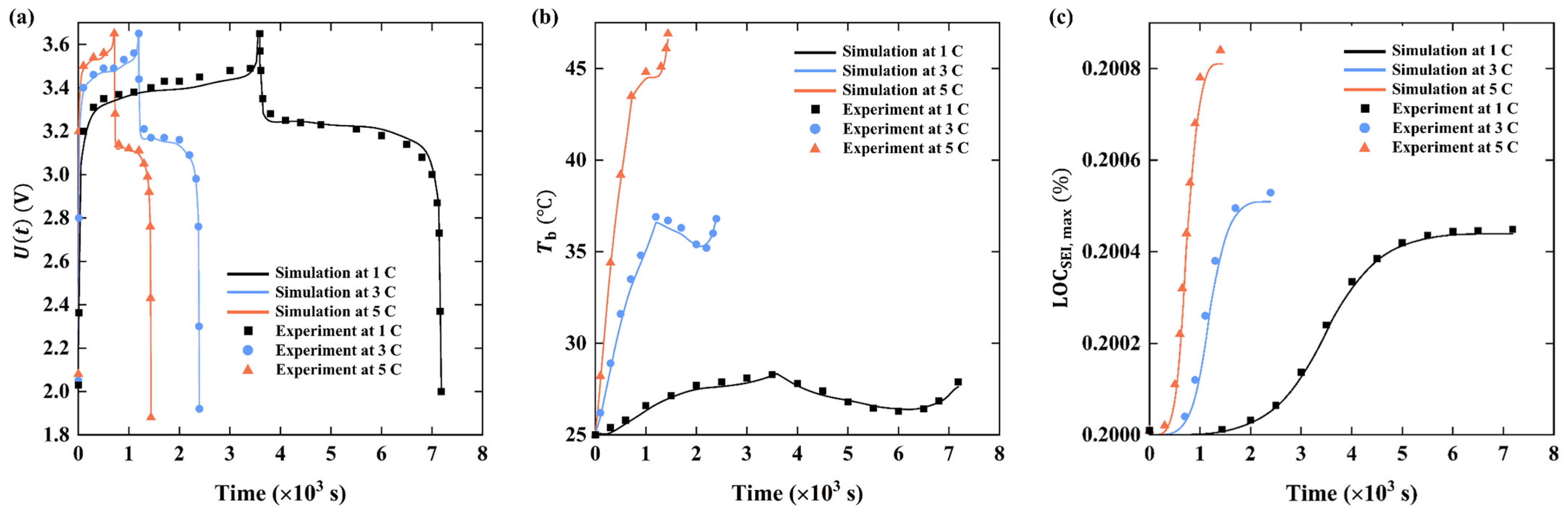
It can be observed from Figure 2b that the thermal management system of the 6s4p battery pack has a certain symmetry. The input parameters into the coupled model are the current and ambient temperature, and the output parameters are the voltage and temperature of the cell. The temperature of battery 6 is the highest due to its structural design. Therefore, batteries 5 and 6 were selected as the key batteries for the study of the cooling strategy. The thermal models of batteries 5 and 6 are shown in Figure 3a. It can be observed that the thermal models are extremely complicated due to the consideration of various thermal terms. However, the thermal model of a single battery is suitable for linearization under certain conditions, as shown in Figure 3b. Moreover, the heat generation of each cell is the same due to the use of the same coupled model and initial conditions, as shown in Figure 3c. Only the heat generation of the cell and the heat transfer with the coolant are considered; a similar simplification can be found in the literature [44].

Based on the above model description and Figure 2b, battery 5 was selected for analysis of the cooling optimization strategy (see Figure 3b) and the thermal model can be expressed as:

$$Q_{\mathrm{b}5}=m_{\mathrm{b}}{C}_{\mathrm{p},\mathrm{b}}\frac{d}{dt}{T}_{\mathrm{b}5}=Q_{\mathrm{gen},\mathrm{b}5}-Q_{\mathrm{b}5-\mathrm{co}},$$

(24)

where $Q_{\mathrm{b}5}$, $Q_{\mathrm{gen},\mathrm{b}5}$, and $Q_{\mathrm{b}5-\mathrm{co}}$ are the heat change, heat generation, and heat transferred from battery 5 to the coolant, respectively. According to the thermal model description and Equation (22), $Q_{\mathrm{gen},\mathrm{b}5}$ can be simplified to:

$$Q_{\mathrm{gen},\mathrm{b}5}=Q_{\mathrm{gen},\mathrm{b}5}=U_{\mathrm{ir}}I+U_{\mathrm{r}}I{T}_{\mathrm{b}5},$$

(25)

where subscripts ir and r represent irreversible and reversible, respectively. $Q_{\mathrm{b}5-\mathrm{co}}$ can be expressed as:

$$Q_{\mathrm{b}5-\mathrm{co}}=h_{\mathrm{b}5-\mathrm{co}}{A}_{\mathrm{b}5-\mathrm{co}}\left(T_{\mathrm{b}5}-T_{\mathrm{co}}\right),$$

(26)

where $h_{\mathrm{b}5-\mathrm{co}}$ and $A_{\mathrm{b}5-\mathrm{co}}$ are the heat transfer coefficient and the contact area between battery 5 and the coolant, respectively. $T_{\mathrm{b}5}$ and $T_{\mathrm{co}}$ are the temperature of battery 5 and the coolant, respectively. The heat transfer coefficient, $h_{\mathrm{b}5-\mathrm{co}}$, can be calculated as [55]:

$$h_{\mathrm{b}5-\mathrm{co}}=\frac{N{u}_{\mathrm{co}}·k_{\mathrm{co}}}{D},$$

(27)

where $N{u}_{\mathrm{co}}$ and $k_{\mathrm{co}}$ are the Nusselt number and the thermal conductivity of coolant, respectively. $D$ is the equivalent diameter of the pipe, which is 35 mm. For the forced convection between the coolant and battery 5, turbulent flow is considered when the length of the pipe is much longer. Thus, $N{u}_{\mathrm{co}}$ can be obtained by the experimental correlation of Sieder–Tate [56]:

$$N{u}_{\mathrm{co}}=0.027{\left(R{e}_{\mathrm{co}}\right)}^{0.8}{\left(P{r}_{\mathrm{co}}\right)}^{\frac{1}{3}}{\left(\frac{{\mu }_{\mathrm{co}}}{{\mu }_{\mathrm{w}}}\right)}^{0.14},$$

(28)

where $R{e}_{\mathrm{co}}$ and $P{r}_{\mathrm{co}}$ are the Reynolds number and Prandtl number of the coolant, respectively. ${\mu }_{\mathrm{co}}$ is the dynamic viscosity of the coolant and ${\mu }_{\mathrm{w}}$ is the dynamic viscosity near the pipe wall. $R{e}_{\mathrm{co}}$ can be calculated as:

$$R{e}_{\mathrm{co}}=\frac{{\rho }_{\mathrm{co}}{v}_{\mathrm{co}}D}{{\mu }_{\mathrm{co}}},$$

(29)

where ${\rho }_{\mathrm{co}}$ and $v_{\mathrm{co}}$ are the density and flow velocity of the coolant, respectively. From Equations (27)–(29), the heat transfer coefficient, $h_{\mathrm{b}5-\mathrm{co}}$, can be expressed as:

$$h_{\mathrm{b}5-\mathrm{co}}=\frac{0.027{\left(R{e}_{\mathrm{co}}\right)}^{0.8}{\left(P{r}_{\mathrm{co}}\right)}^{\frac{1}{3}}{\left(\frac{{\mu }_{\mathrm{co}}}{{\mu }_{\mathrm{w}}}\right)}^{0.14}{k}_{\mathrm{co}}}{D}=a_1{v}_{\mathrm{co}}{}^{0.8},$$

(30)

where $a_1=\frac{0.027{\left({\rho }_{\mathrm{co}}\right)}^{0.8}{\left(P{r}_{\mathrm{co}}\right)}^{\frac{1}{3}}{k}_{\mathrm{co}}}{{\left({\mu }_{\mathrm{co}}\right)}^{0.66}{\left({\mu }_{\mathrm{w}}\right)}^{0.14}{D}^{0.2}}$. Let $u=v_{\mathrm{co}}{}^{0.8}$, from Equations (24)–(30), then the temperature of battery 5 ($T_{\mathrm{b}5}$) can be expressed as:

$$\frac{d}{dt}{T}_{\mathrm{b}5}=\frac{U_{\mathrm{ir}}I+U_{\mathrm{r}}I{T}_{\mathrm{b}5}}{m_{\mathrm{b}}{C}_{\mathrm{p},\mathrm{b}}}-\frac{a_1{A}_{\mathrm{b}5-\mathrm{co}}\left(T_{\mathrm{b}5}-T_{\mathrm{co}}\right)}{m_{\mathrm{b}}{C}_{\mathrm{p},\mathrm{b}}}u$$

(31)

The input is the current load, $I$, and the coolant flow rate, $v$, and the output is the temperature of battery 5.

As mentioned above, a new cooling and control strategy should be proposed to avoid too much cooling or an excessive increase in battery temperature. Fortunately, a thermal model of a single battery is available for the design of triple-step nonlinear cooling control. After the triple-step nonlinear cooling control strategy was solved for battery 5, this strategy was applied to the 6s4p battery pack to validate its applicability. Moreover, an extended PID cooling control strategy was also adopted to compare the results with those using a triple-step nonlinear cooling control strategy. Both the triple-step nonlinear method and extended PID method adjust the temperature of battery 5 by changing the coolant flow rate. The detailed design process is shown in Figure 4.

The design of steady state control, the reference variable feed-forward control, and the error feedback control are three main steps of the triple-step nonlinear method [44,57]. The design processes for battery 5 are illustrated in Figure 3d,e, respectively. $T_{\mathrm{tv}}$ is the target temperature of battery 5, $T_{\mathrm{b}5}$ is the actual temperature of battery 5, and $u$ is a control law. Let $A\left(T_{\mathrm{b}5}\right)=\frac{U_{\mathrm{ir}}I+U_{\mathrm{r}}I{T}_{\mathrm{b}5}}{m_{\mathrm{b}}{C}_{\mathrm{p},\mathrm{b}}}$, $B\left(T_{\mathrm{b}5}\right)=-\frac{a_1{A}_{\mathrm{b}5-\mathrm{co}}\left(T_{\mathrm{b}5}-T_{\mathrm{co}}\right)}{m_{\mathrm{b}}{C}_{\mathrm{p},\mathrm{b}}}$. Then, Equation (31) can be rewritten as:

$$\frac{d}{dt}{T}_{\mathrm{b}5}=A\left(T_{\mathrm{b}5}\right)+B\left(T_{\mathrm{b}5}\right)u$$

(32)

Equation (32) can be adapted to different methods [58].

Step 1: Steady-state-like Control.

The control law, $u_{\mathrm{s}}$, changes dynamically with the output. The purpose of $u_{\mathrm{s}}$ is to gradually adjust the temperature of battery 5 to a stable state. When a stable state is reached, $\frac{d}{dt}{T}_{\mathrm{b}5}=0$, so combining Equations (31) and (32), we then obtain:

$$u_{\mathrm{s}}=-\frac{A\left(T_{\mathrm{b}5}\right)}{B\left(T_{\mathrm{b}5}\right)}=\frac{U_{\mathrm{ir}}I+U_{\mathrm{r}}I{T}_{\mathrm{b}5}}{a_1{A}_{\mathrm{b}5-\mathrm{co}}\left(T_{\mathrm{b}5}-T_{\mathrm{co}}\right)},B\left(T_{\mathrm{b}5}\right)\ne 0$$

(33)

Step 2: Reference Variable Feed-forward Control.

The target temperature, $T_{\mathrm{tv}}$, is pre-set and has a prediction effect on its differential, $\frac{d}{dt}{T}_{\mathrm{tv}}$. Therefore, introducing the tracking target temperature control law can effectively reduce the adjustment time. The control law, $u_{\mathrm{f}}$, is added based on Step 1. By letting $\frac{d}{dt}{T}_{\mathrm{b}5}=\frac{d}{dt}{T}_{\mathrm{tv}}$, we obtain:

$$u=u_{\mathrm{s}}+u_{\mathrm{f}}\to u_{\mathrm{f}}=\frac{1}{B\left(T_{b5}\right)}·\frac{d}{dt}{T}_{\mathrm{tv}}=-\frac{m_{\mathrm{b}}{C}_{\mathrm{p},\mathrm{b}}}{a_1{A}_{\mathrm{b}5-\mathrm{co}}\left(T_{\mathrm{b}5}-T_{\mathrm{co}}\right)}·\frac{d}{dt}{T}_{\mathrm{tv}}$$

(34)

Step 3: Error Feedback Control.

Based on the controller design method of the error system, the control law, $u_{\mathrm{e}}$, is obtained. This control law can further reduce the impact caused by the external disturbance and modeling deviation of the system and guarantee the steady-state of the system.

$$u=u_{\mathrm{s}}+u_{\mathrm{f}}+u_{\mathrm{e}}\to u_{\mathrm{e}}=-\frac{1}{B\left(T_{\mathrm{b}5}\right)}\left(\frac{d}{dt}{T}_{\mathrm{tv}}-\frac{d}{dt}{T}_{\mathrm{b}5}\right)$$

(35)

The error is the deviation between the target temperature and actual temperature of battery 5:

$$\mathrm{e}=T_{\mathrm{tv}}-T_{\mathrm{b}5}$$

(36)

Based on Equations (35) and (36), the derivative of the input deviation can be expressed as:

$$\frac{d}{dt}\mathrm{e}=-B\left(T_{\mathrm{b}5}\right)u_{\mathrm{e}}$$

(37)

The Lyapunov function is selected to solve the error feedback control law [44]:

$$V=\frac{1}{2}{\mathrm{e}}^2+\frac{1}{2}{K}_0{\left(\int \mathrm{e}dt\right)}^2\to \frac{d}{dt}V=\mathrm{e}·\frac{d}{dt}\mathrm{e}+K_0\mathrm{e}\int \mathrm{e}dt$$

(38)

Let $\frac{d}{dt}V=-K_1{\mathrm{e}}^2$, and combine Equations (37) and (38), then the control law can be expressed as:

$$-B\left(T_{\mathrm{b}5}\right)·u_{\mathrm{e}}=-K_1\mathrm{e}-K_0\int \mathrm{e}dt$$

(39)

where $K_1>0$ and $K_0>0$. When $\frac{d}{dt}V\le 0$, a stable state is achieved. By simplifying Equation (39), the control law can be expressed as:

$$\begin{array}{l}{u}_{\mathrm{e}}=\frac{K_1\mathrm{e}}{B\left(T_{\mathrm{b}5}\right)}+\frac{K_0}{B\left(T_{\mathrm{b}5}\right)}\int \mathrm{e}dt\to u_{\mathrm{e}}\\ =-\frac{m_{\mathrm{b}}{C}_{\mathrm{p},\mathrm{b}}{K}_1}{a_1{A}_{\mathrm{b}5-\mathrm{co}}\left(T_{\mathrm{b}5}-T_{\mathrm{co}}\right)}\mathrm{e}-\frac{m_{\mathrm{b}}{C}_{\mathrm{p},\mathrm{b}}{K}_0}{a_1{A}_{\mathrm{b}5-\mathrm{co}}\left(T_{\mathrm{b}5}-T_{\mathrm{co}}\right)}\int \mathrm{e}dt\end{array}$$

(40)

Equations (33), (34), and (40) are summarized as the final control law:

$$u=-\frac{A\left(T_{\mathrm{b}5}\right)}{B\left(T_{\mathrm{b}5}\right)}+\frac{1}{B\left(T_{\mathrm{b}5}\right)}·\frac{d}{dt}{T}_{\mathrm{tv}}+\frac{K_1\mathrm{e}}{B\left(T_{\mathrm{b}5}\right)}+\frac{K_0}{B\left(T_{\mathrm{b}5}\right)}\int \mathrm{e}dt$$

(41)

The final control law is:

$$\begin{array}{c}u=\frac{U_{\mathrm{ir}}I+U_{\mathrm{r}}I{T}_{\mathrm{b}5}}{a_1{A}_{\mathrm{b}5-\mathrm{co}}\left(T_{\mathrm{b}5}-T_{\mathrm{co}}\right)}-\frac{m_{\mathrm{b}}{C}_{\mathrm{p},\mathrm{b}}}{a_1{A}_{\mathrm{b}5-\mathrm{co}}\left(T_{\mathrm{b}5}-T_{\mathrm{co}}\right)}·\frac{d}{dt}{T}_{\mathrm{tv}}-\frac{m_{\mathrm{b}}{C}_{\mathrm{p},\mathrm{b}}{K}_1}{a_1{A}_{\mathrm{b}5-\mathrm{co}}\left(T_{\mathrm{b}5}-T_{\mathrm{co}}\right)}\mathrm{e}\\ -\frac{m_{\mathrm{b}}{C}_{\mathrm{p},\mathrm{b}}{K}_0}{a_1{A}_{\mathrm{b}5-\mathrm{co}}\left(T_{\mathrm{b}5}-T_{\mathrm{co}}\right)}\int \mathrm{e}dt\end{array}$$

(42)

We now consider the system modeling error, $\mathrm{d}$i. Under the framework of state stability theory, the robust stability of the system needs to be analyzed. Let $\zeta =\int \mathrm{e}dt$, then combining Equations (37) and (39), we obtain:

$$\mathrm{e}=\dot{\zeta }\to \frac{d\mathrm{e}}{dt}=-K_1\mathrm{e}-K_0\zeta +\mathrm{di},$$

(43)

and Equation (43) can be expressed in the matrix form as:

$$\frac{d\overline{\mathrm{e}}}{dt}=H\overline{\mathrm{e}}+G\mathrm{di},$$

(44)

where $\overline{\mathrm{e}}={\left[\xi \mathrm{e}\right]}^T$, $H=\left[\begin{array}{c}0\\ -K_0\end{array} \begin{array}{c}1\\ -K_1\end{array}\right]$, and $G={\left[0 1\right]}^T$. Equation (44) is a linear system. As mentioned above, in the description of the triple-step nonlinear method, the asymptotic stability of the system is demonstrated without considering the disturbance, $\mathrm{di}$. According to the conclusion of input state stability of a linear system, the closed-loop system has robust stability [59].

3. Model Validation

The whole system is established in the one-dimensional software package AMESim, including the electrochemical model, thermal model, aging model, and cooling control model. Each module provided by AMESim is modeled based on physical mechanisms. The connection relationship between the modules in the system is stated in the above description, and the practicability of each module has been proven through extensive research [44,45,58]. Therefore, AMESim is an experimental platform that can be used to replace the real experimental platform to explore the battery performance in the thermal management system. Moreover, the model of a 5 $\mathrm{A}·\mathrm{h}$ LFP/C battery at 25 °C was adopted for the validation of the battery model used in this study, as shown in Figure 5. The equipment used in the experiment has been introduced in previous work [51]. In this work, a cycle consists of a constant-current (CC) charging process and a constant-current discharging process. The experimental charge–discharge data were then compared with the simulated results in this study, as shown in Figure 6.

Figure 6a shows the voltage curves of the charge–discharge process at different C-rates. It can be seen that the simulated curves agree well with the experimental results. Then, the experimental temperature data at different C-rates were then compared with the simulated results, as shown in Figure 6b. The cell temperature can reach 47.5 °C at five C-rates after one cycle of the charge–discharge process. The temperature curves obtained by simulation at different C-rates were also in good agreement with the experimental values. Finally, the decrease in capacity was compared and validated. The aging mechanism of the SEI formation was considered in the simulations for all conditions. The initial capacity loss, $C_{\mathrm{loss},\mathrm{int}}^{\mathrm{SEI}}$, was 0.01 $\mathrm{A}·\mathrm{h}$ according to the battery factory parameters, which was set as the initial condition in the modeling, as shown in Table 6. The loss of capacity (LOC) (the ratio of the lost capacity to nominal capacity, 5 $\mathrm{A}·\mathrm{h}$) was calculated by Equation (44) at different C-rates, and then compared with the experimental data, as shown in Figure 6c. The comparison presents good agreement, which indicates the model accuracy. The simulated results were slightly different from the experimental data, which was possibly due to some model parameters not being totally applicable to the experimental tests. In addition, the initial conditions and boundary conditions of the battery in the experiment and simulation are not exactly the same. The simulated battery temperature was also compared with that in the literature [32,60] during the charge–discharge process, showing a good agreement. For example, the battery temperature in Figure 6b is verified in the literature [32].

4. Results and Discussion

4.1. Performance of Battery Cell and 6s4p Battery Pack under Natural Cooling

The thermal behavior and aging performance of a battery cell and the 6s4p battery pack were first investigated under natural cooling. The charge–discharge process of a single cell was first charged and then discharged and cycled at different C-rates and ambient temperatures ($T_{\mathrm{amb}}$). The temperature and LOC evolutions of a single cell are shown in Figure 7. Taking the time required for one charge–discharge cycle at one C-rate as the standard, Figure 7a,b shows the battery temperature and LOC at C-rates from one to five. As the C-rate increases, the time for a single charge–discharge cycle becomes shorter, so the number of cycles increases. It can be observed that both the battery temperature and LOC increase with the increase in the C-rate. The maximum battery temperature can even exceed 50 °C at a C-rate of five, which is essentially consistent with the results of our previous research [32]. The LOC continues to increase as the charge–discharge cycles proceed, and also correspondingly increases with the increasing C-rate. The initial LOC is 0.01 $\mathrm{A}·\mathrm{h}$, accounting for 0.2%. The final LOC exceeds 0.21% at a C-rate of five, which means that the newly added LOC reaches 0.01% after only about five charge–discharge cycles. For a C-rate of five, the evolutions of battery temperature and LOC at different $T_{\mathrm{amb}}$ are presented, as shown in Figure 7c,d. Both the battery temperature and LOC increase when the $T_{\mathrm{amb}}$ increases from 25 °C to 65 °C. The maximum battery temperature and LOC can even reach 80 °C and 1% at $T_{\mathrm{amb}}=65 ℃$, respectively. A thermal runaway can occur in a battery cell when the temperature exceeds 80 °C, which is beyond the scope of this study. Therefore, both the C-rate and $T_{\mathrm{amb}}$ are critical for the thermal behavior and aging performance of a battery cell.

Before studying the thermal behavior and aging performance of the 6s4p battery pack, the temperature and aging performance of a single cell are further summarized and analyzed. The temperature, LOC, SEI layer thickness, and SEI layer porosity of a single battery at different C-rates and ambient temperatures are shown in Figure 8. As shown in the figures, the C-rate plays an important role in the thermal behavior during the charge–discharge process of the battery cell. Moreover, the temperature rise is relatively uniform with the $T_{\mathrm{amb}}$ increasing from 25 °C to 65 °C, regardless of the C-rate. This indicates that although the battery temperature is greatly affected by the $T_{\mathrm{amb}}$, the difference in the effect under different C-rates is small, as shown in Figure 8a. However, this situation is not the same for the aging performance of the battery cell, as shown in Figure 8b–d. As the C-rate and $T_{\mathrm{amb}}$ increase, the uptrend of LOC, SEI layer thickness, and SEI layer porosity is slow at first and then sharp. It reveals that the high C-rate and $T_{\mathrm{amb}}$ extensively accelerate the battery aging, while normal C-rate and $T_{\mathrm{amb}}$ have less effect. Since the initial LOC is considered to be 0.2% (0.01 $\mathrm{A}·\mathrm{h}$), the initial SEI layer thickness and porosity are, 4.03848 nm and 0.01, respectively.

Based on the above analysis, the thermal behavior and aging performance of the 6s4p battery under natural cooling are then studied. The heat conduction between battery cells and heat convection and radiation between the cell and ambient air are considered. The evolutions of maximum battery temperature, LOC, SEI layer thickness, and SEI layer porosity in the 6s4p battery pack at $T_{\mathrm{amb}}=25℃$ are shown in Figure 9. The maximum battery temperature in the 6s4p battery pack can reach 80 °C at 5 C-rate, even if the $T_{\mathrm{amb}}$ is only 25 °C, as shown in Figure 9a. This means that the rapid heat generation of the battery pack at a high C-rate leads to a sharp increase in temperature, which requires the intervention of a thermal management system for timely cooling and heat dissipation. In addition, the SEI formation continuously occurs, resulting in the continuous increase of SEI layer thickness and porosity, and thus the LOC of the battery. Specifically, the maximum and minimum temperature, LOC, SEI layer thickness, and SEI layer porosity of the cells in the 6s4p battery pack at different C-rates are shown in Figure 10. As shown in the figures, squares of different styles and colors represent different meanings. Where green represents the initial value, red represents the maximum value, and blue represents the minimum value. The increase of the C-rate has a linear effect on the battery temperature, while the effect on the aging performance has a sudden change. The aging at low C-rates is small or even negligible (such as 1 C and 2 C), but the aging at high C-rates is not negligible (such as 4 C and 5 C).

4.2. Performance of 6s4p Battery Pack under Two Modes Cooling System

After exploring the performance of the 6s4p battery pack under natural cooling, the thermal behavior and aging performance of the 6s4p battery pack in two cooling modes are further investigated and compared. For both parallel and series cooling, the pump rotary speeds of 1000 and 3000 $\mathrm{r}·{\min }^{-1}$ are considered to provide the kinetic energy for coolant. According to the pump performance in the AMESim, the corresponding mechanical power provided by the pump to the coolant is 7.168 W and 218.873 W, and 2.620 W and 81.552 W under parallel and series cooling, respectively, as shown in Table 7. This indicates that parallel cooling is more energy efficient while series cooling requires a higher pump rotary speed to obtain the power. Further, the volumetric flow rate and velocity of the coolant can be obtained. It is worth mentioning that the flow in the four cold plates is the same under parallel cooling, which means a quarter of the total flow rate in each cold plate, as shown in Table 7. Therefore, for parallel cooling, the mass flow rates of each cold plate are, respectively, 0.081 and 0.276 $\mathrm{kg}·{\mathrm{s}}^{-1}$ when the pump rotary speeds are 1000 and 3000 $\mathrm{r}·{\min }^{-1}$. For series cooling, the mass flow rates of each cold plate are always, respectively, 0.118 and 0.408 $\mathrm{kg}·{\mathrm{s}}^{-1}$. Combining the C-rates from 1 to 5, 20 cases (cases A to T) can be divided, as shown in Table 7.

Figure 11a,b show the evolutions of the maximum battery temperature in the 6s4p battery pack for the 20 cases. For both parallel and series cooling, the ambient temperature is set to 25 °C. Overall, under the same C-rate and coolant flow rate, the maximum battery temperature of the series and parallel cooling systems is close. From the specific values obtained from the simulation, the maximum battery temperature in the series connection is slightly higher. In addition, it is noteworthy that the maximum battery temperature in the 6s4p battery pack does not always decrease with the coolant flow rate increases. This phenomenon is particularly evident in parallel cooling, as shown in Figure 11a. When the C-rate is high, such as 4 C and 5 C, the heat generation of the battery is higher. A Larger coolant flow rate allows for faster heat exchange and more heat removal. Therefore, the maximum battery temperature at a higher coolant flow rate (Case F and G) is lower than that at a lower coolant flow rate (Case A and B). The opposite situation occurs when the C-rate is low, such as 1 C and 2 C. The battery does not generate much heat at this time, and a smaller coolant flow rate can carry out heat exchange for a longer time. Therefore, the maximum battery temperature at a lower coolant flow rate (Case D and E) is lower than that at a higher coolant flow rate (Case I and J). Further, the evolutions of the maximum temperature difference in the 6s4p battery pack for the 20 cases, as shown in Figure 11c,d. It can be observed that the maximum temperature difference in the 6s4p battery pack decreases with the coolant flow rate increasing, regardless of the C-rate. As the coolant flow rate increases, the maximum temperature difference decreases more with parallel cooling than that with series cooling. This indicates that increasing the coolant flow rate can better reduce the temperature difference between the cells in the battery pack when parallel cooling is used. These results also demonstrate that at a high C-rate, a further increase in the coolant flow rate is required to control the temperature and temperature difference of the battery pack. Furthermore, parallel cooling is relatively more advantageous.

Based on the above analysis, the temperature, LOC, SEI layer thickness, and SEI layer porosity of the cells in the 6s4p battery pack under parallel cooling are further analyzed. After the charge–discharge process, the maximum and minimum battery temperatures at high and low coolant flow rates are calculated at different C-rates, as shown in Figure 12a. For high C-rates (4 C and 5 C), the maximum and minimum temperature at a higher coolant flow rate (0.276 $\mathrm{kg}·{\mathrm{s}}^{-1}$) is lower than those at a lower coolant flow rate (0.081 $\mathrm{kg}·{\mathrm{s}}^{-1}$). For low C-rates (1 C and 2 C), the maximum and minimum temperatures at a higher coolant flow rate are higher than those at a lower coolant flow rate. These results also validate the results in Figure 11. Further, the characteristics of this change caused by the difference in C-rate and coolant flow rate are also reflected in the parameters of battery aging, as shown in Figure 12b–d. The use of a higher coolant flow rate at high C-rates can not only reduce the maximum temperature of the battery pack but also reduce the formation of SEI, thereby reducing capacity loss. Moreover, applying a higher coolant flow rate at low C-rates, not only is the optimization of battery temperature and aging performance not as good as those at a lower coolant flow rate, but a higher coolant flow rate also consumes more pump power. Therefore, high coolant flow is required at high C-rates, and low coolant flow is more suitable at low C-rates. All these show that it is necessary to select the appropriate coolant flow to ensure the performance of the battery. This requires timely adjustment of the coolant flow rate according to the working conditions of the battery.

4.3. Cooling Optimization of 6s4p Battery Pack under Different Cycle Conditions

As mentioned above, the triple-step nonlinear cooling control strategy is first solved for a single cell, and then this strategy is applied to the 6s4p battery pack to validate its applicability. Moreover, an extended PID cooling control strategy is also adopted to compare the results with those using a triple-step nonlinear cooling control strategy. Both the triple-step nonlinear method and the extended PID method adjust the temperature by changing the coolant flow rate. The effect of two methods is verified under constant current (2 C-rate), New European Driving Cycle (NEDC), and Urban Severe Driving Cycle (US06). Each working condition circulates two times to test the effect of control and optimization. NEDC consists of 4 urban cycles and 1 suburban cycle, and US06 represents an aggressive driving cycle. The initial temperature of the 6s4p battery pack is 40 °C, and the temperature of coolant and ambient is 25 °C.

Under 2 C-rate charge–discharge cycles, the heat generation of each battery cell is shown in Figure 13a. It can be seen that the heat generation in the discharge process is higher than that in the charging process. At the end of the charge and discharge process, the heat generation increases sharply. The well-tuned four parameters of the extended PID method are: $K_{ip}=2\times {10}^{-4}$ (inner proportional element), $K_p=6\times {10}^{-2}$ (proportional element), $K_i=2\times {10}^{-6}$ (integral element), $K_d=1\times {10}^{-4}$ (derivative element). The comparison of coolant velocity under extended PID and triple-step nonlinear control is shown in Figure 13b. The coolant velocity increases continuously as the charge–discharge proceeds under the extended PID control, while under the triple-step nonlinear control, the coolant velocity increases smoothly. This indicates less pump power under the triple-step nonlinear control. The temperature comparison of battery 6, battery 5, and cold plate under extended PID and triple-step nonlinear control is shown in Figure 13c. As can be seen from the figure, under the triple-step nonlinear control, the temperature of the cold plate can be controlled at about 25 °C in a short time, while the extended PID control takes a little more time, which verifies the validity of the triple-step nonlinear method. Further, through the temperature evolution of batteries 5 and 6, the application effect of the two control methods in the 6s4p battery pack can be analyzed. The temperature of batteries 6 and 5 can be controlled to be below 35 °C and 32 °C in about 10 min, respectively. Although the subsequent charge–discharge process causes some temperature fluctuations, the temperature of batteries 6 and 5 can still be controlled below 34 °C and 31 °C, respectively. In addition, whether it is the temperature of the battery or the cold plate, the difference between the two methods is small, and the triple-step nonlinear method has a slight advantage. This slight advantage can be inferred from the aging performance of the batteries, as shown in Figure 13d. The LOC of batteries 6 and 5 under triple-step nonlinear control is smaller than that under the extended PID control.

Under NEDC cycles, the heat generation of each battery cell is shown in Figure 14a. The heat generation also increases dramatically at the end of each urban and suburban cycle. The well-tuned four parameters of the extended PID method are: $K_{ip}=3\times {10}^{-3}$, $K_p=1\times {10}^{-2}$, $K_i=2\times {10}^{-8}$, $K_d=1\times {10}^{-4}$. The comparison of coolant velocity under extended PID and triple-step nonlinear control is shown in Figure 14b. The coolant velocity increases continuously under the extended PID control, while under the triple-step nonlinear control, the coolant velocity correspondingly changes with the change of heat generation. This indicates a more efficient control of coolant flow rate and less pump power consumption under the triple-step nonlinear control. The temperature comparison of battery 6, battery 5, and the cold plate is also shown in Figure 14c. The triple-step nonlinear method still shows a good control effect on the temperature of the cold plate. The temperature of batteries 6 and 5 can be controlled to be below 34 °C and 32 °C in about 6 min, respectively. During the subsequent cycle, the temperature of batteries 6 and 5 can further be controlled to be below 29 °C and 28 °C, respectively. The triple-step nonlinear method still has a slight advantage, which can be inferred from the aging performance of the batteries, as shown in Figure 14d.

Under US06 cycles, the heat generation of each battery cell is shown in Figure 15a. The aggressive driving cycles lead to dramatic and fluctuating heat generation. The well-tuned four parameters of the extended PID method are: $K_{ip}=3\times {10}^{-3}$, $K_p=1.5\times {10}^{-2}$, $K_i=2\times {10}^{-7}$, $K_d=1\times {10}^{-4}$. The comparison of coolant velocity under extended PID and triple-step nonlinear control is shown in Figure 15b. The coolant velocity still increases continuously under the extended PID control, while under the triple-step nonlinear control, the coolant velocity correspondingly fluctuates with the change of the heat generation. This also indicates a more efficient control of coolant flow rate and less pump power consumption under the triple-step nonlinear control. The temperature comparison of battery 6, battery 5, and the cold plate is also shown in Figure 15c. The triple-step nonlinear method still shows a good control effect on the temperature of the cold plate. The temperature of batteries 6 and 5 can be controlled to be below 38 °C and 34 °C in about 9 min, respectively. During the subsequent cycle, the temperature of batteries 6 and 5 can further be controlled to be below 36 °C and 32 °C, respectively. The triple-step nonlinear method still has a slight advantage, which can be inferred from the aging performance of the batteries, as shown in Figure 15d.

5. Conclusions

Two modes of thermal management system for 6s4p battery pack are established based on one-dimensional modeling. The single particle model with the consideration of aging is adopted for the battery. Both the battery temperature and loss of capacity (LOC) increase when the C-rate and ambient temperature ($T_{\mathrm{amb}}$) increase. The maximum battery temperature and LOC can even reach 80 °C and 1% at $T_{\mathrm{amb}}=65 ℃$, respectively. High C-rate and $T_{\mathrm{amb}}$ can extensively accelerate the battery aging, while normal C-rate and $T_{\mathrm{amb}}$ have weaker effect. The maximum battery temperature in the 6s4p battery pack can reach 80 °C at 5 C-rate, even if the $T_{\mathrm{amb}}$ is only 25 °C. The comparison of pump power, thermal behavior, and aging performance indicate parallel cooling is relatively more advantageous. When the C-rate is high (4 C and 5 C), the maximum battery temperature at a higher coolant flow rate (0.276 $\mathrm{kg}·{\mathrm{s}}^{-1}$) is lower than that at a lower coolant flow rate (0.081 $\mathrm{kg}·{\mathrm{s}}^{-1}$). When the C-rate is low (1 C and 2 C), the maximum battery temperature at a lower coolant flow rate is lower than that at a higher coolant flow rate. The characteristics of this change caused by the difference in C-rate and coolant flow rate are also reflected in the battery aging. Further, a cooling control strategy for the key battery is firstly proposed based on the triple-step nonlinear method, and then the optimization effect of this strategy in the battery pack is validated under 2 C charge–discharge cycles, NEDC cycles, and US06 cycles. Moreover, the extended PID control strategy is constructed and compared with the triple-step nonlinear method. The results show that the temperature and LOC of key batteries and the temperature of the cold plate are lower than that of the extended PID method. This verifies the validity of the triple-step nonlinear method and shows an advantage compared with the extended PID method.

References

1. Al-Zareer, M.; Dincer, I.; Rosen, M.A. A Review of Novel Thermal Management Systems for Batteries. Int. J. Energy Res. 2018, 42, 3182–3205. [Google Scholar] [CrossRef]
2. Patil, M.S.; Seo, J.H.; Panchal, S.; Jee, S.W.; Lee, M.Y. Investigation on Thermal Performance of Water-Cooled Li-Ion Pouch Cell and Pack at High Discharge Rate with U-Turn Type Microchannel Cold Plate. Int. J. Heat Mass Transf. 2020, 155, 119728. [Google Scholar] [CrossRef]
3. Panchal, S.; Gudlanarva, K.; Tran, M.K.; Fraser, R.; Fowler, M. High Reynold’s Number Turbulent Model for Micro-Channel Cold Plate Using Reverse Engineering Approach for Water-Cooled Battery in Electric Vehicles. Energies 2020, 13, 1638. [Google Scholar] [CrossRef] [Green Version]
4. Ye, M.; Guo, H.; Xiong, R.; Yu, Q. A Double-Scale and Adaptive Particle Filter-Based Online Parameter and State of Charge Estimation Method for Lithium-Ion Batteries. Energy 2018, 144, 789–799. [Google Scholar] [CrossRef]
5. Tran, M.K.; Panchal, S.; Chauhan, V.; Brahmbhatt, N.; Mevawalla, A.; Fraser, R.; Fowler, M. Python-Based Scikit-Learn Machine Learning Models for Thermal and Electrical Performance Prediction of High-Capacity Lithium-Ion Battery. Int. J. Energy Res. 2022, 46, 786–794. [Google Scholar] [CrossRef]
6. Hekmat, S.; Molaeimanesh, G.R. Hybrid Thermal Management of a Li-Ion Battery Module with Phase Change Material and Cooling Water Pipes: An Experimental Investigation. Appl. Therm. Eng. 2020, 166, 114759. [Google Scholar] [CrossRef]
7. Li, L.; Chen, X.; Yuan, Q.; Wang, T.; Ji, H.; Papović, S.; Raleva, K.; Pan, F.; Yang, T.; Li, J. Effects of Minor Mechanical Deformation on the Lifetime and Performance of Commercial 21700 Lithium-Ion Battery. J. Electrochem. Soc. 2022, 169, 060544. [Google Scholar] [CrossRef]
8. Latini, D.; Vaccari, M.; Lagnoni, M.; Orefice, M.; Mathieux, F.; Huisman, J.; Tognotti, L.; Bertei, A. A Comprehensive Review and Classification of Unit Operations with Assessment of Outputs Quality in Lithium-Ion Battery Recycling. J. Power Sources 2022, 546, 231979. [Google Scholar] [CrossRef]
9. Ghaeminezhad, N.; Wang, Z.; Ouyang, Q. A Review on Lithium-Ion Battery Thermal Management System Techniques: A Control-Oriented Analysis. Appl. Therm. Eng. 2023, 219, 119497. [Google Scholar] [CrossRef]
10. Wu, W.; Wang, S.; Wu, W.; Chen, K.; Hong, S.; Lai, Y. A Critical Review of Battery Thermal Performance and Liquid Based Battery Thermal Management. Energy Convers. Manag. 2019, 182, 262–281. [Google Scholar] [CrossRef]
11. Kim, J.; Oh, J.; Lee, H. Review on Battery Thermal Management System for Electric Vehicles. Appl. Therm. Eng. 2019, 149, 192–212. [Google Scholar] [CrossRef]
12. Aswin Karthik, C.; Kalita, P.; Cui, X.; Peng, X. Thermal Management for Prevention of Failures of Lithium Ion Battery Packs in Electric Vehicles: A Review and Critical Future Aspects. Energy Storage 2020, 2, e137. [Google Scholar] [CrossRef] [Green Version]
13. Lin, J.; Liu, X.; Li, S.; Zhang, C.; Yang, S. A Review on Recent Progress, Challenges and Perspective of Battery Thermal Management System. Int. J. Heat Mass Transf. 2021, 167, 120834. [Google Scholar] [CrossRef]
14. Mohammadian, S.K.; Zhang, Y. Thermal Management Optimization of an Air-Cooled Li-Ion Battery Module Using Pin-Fin Heat Sinks for Hybrid Electric Vehicles. J. Power Sources 2015, 273, 431–439. [Google Scholar] [CrossRef]
15. Mohammadian, S.K.; Rassoulinejad-Mousavi, S.M.; Zhang, Y. Thermal Management Improvement of an Air-Cooled High-Power Lithium-Ion Battery by Embedding Metal Foam. J. Power Sources 2015, 296, 305–313. [Google Scholar] [CrossRef]
16. An, Z.; Shah, K.; Jia, L.; Ma, Y. A Parametric Study for Optimization of Minichannel Based Battery Thermal Management System. Appl. Therm. Eng. 2019, 154, 593–601. [Google Scholar] [CrossRef] [Green Version]
17. Liu, J.; Li, H.; Li, W.; Shi, J.; Wang, H.; Chen, J. Thermal Characteristics of Power Battery Pack with Liquid-Based Thermal Management. Appl. Therm. Eng. 2020, 164, 114421. [Google Scholar] [CrossRef]
18. Mortazavi, B.; Yang, H.; Mohebbi, F.; Cuniberti, G.; Rabczuk, T. Graphene or H-BN Paraffin Composite Structures for the Thermal Management of Li-Ion Batteries: A Multiscale Investigation. Appl. Energy 2017, 202, 323–334. [Google Scholar] [CrossRef] [Green Version]
19. Zhang, W.; Ling, G.; Zhuang, L.; Liang, Z. The Effect of Reducing the Thermal Contact Resistance on the Performance of Battery Thermal Management System. Int. J. Energy Res. 2021, 45, 9970–9982. [Google Scholar] [CrossRef]
20. Liu, F.F.; Lan, F.C.; Chen, J.Q.; Li, Y.G. Experimental Investigation on Cooling/Heating Characteristics of Ultra-Thin Micro Heat Pipe for Electric Vehicle Battery Thermal Management. Chinese J. Mech. Eng. 2018, 31, 53. [Google Scholar] [CrossRef]
21. Zhang, Z.; Wei, K. Experimental and Numerical Study of a Passive Thermal Management System Using Flat Heat Pipes for Lithium-Ion Batteries. Appl. Therm. Eng. 2020, 166, 114660. [Google Scholar] [CrossRef]
22. Li, X.; He, F.; Zhang, G.; Huang, Q.; Zhou, D. Experiment and Simulation for Pouch Battery with Silica Cooling Plates and Copper Mesh Based Air Cooling Thermal Management System. Appl. Therm. Eng. 2019, 146, 866–880. [Google Scholar] [CrossRef]
23. Dan, D.; Yao, C.; Zhang, Y.; Zhang, H.; Zeng, Z.; Xu, X. Dynamic Thermal Behavior of Micro Heat Pipe Array-Air Cooling Battery Thermal Management System Based on Thermal Network Model. Appl. Therm. Eng. 2019, 162, 114183. [Google Scholar] [CrossRef]
24. Zhang, L.; Yuan, Q.; Hu, S.; Xu, X. Research on Performance of Thermal Management System Integrated with Multiple Heat Exchange Methods. Ionics 2022, 28, 789–799. [Google Scholar] [CrossRef]
25. Kabir, M.M.; Demirocak, D.E. Degradation Mechanisms in Li-Ion Batteries: A State-of-the-Art Review. Int. J. Energy Res. 2017, 41, 1963–1986. [Google Scholar] [CrossRef]
26. Xiong, R.; Pan, Y.; Shen, W.; Li, H.; Sun, F. Lithium-Ion Battery Aging Mechanisms and Diagnosis Method for Automotive Applications: Recent Advances and Perspectives. Renew. Sustain. Energy Rev. 2020, 131, 110048. [Google Scholar] [CrossRef]
27. Birkl, C.R.; Roberts, M.R.; McTurk, E.; Bruce, P.G.; Howey, D.A. Degradation Diagnostics for Lithium Ion Cells. J. Power Sources 2017, 341, 373–386. [Google Scholar] [CrossRef]
28. Kamyab, N.; Weidner, J.W.; White, R.E. Mixed Mode Growth Model for the Solid Electrolyte Interface (SEI). J. Electrochem. Soc. 2019, 166, A334–A341. [Google Scholar] [CrossRef]
29. Yang, S.-c.; Hua, Y.; Qiao, D.; Lian, Y.-b.; Pan, Y.-w.; He, Y.-l. A Coupled Electrochemical-Thermal-Mechanical Degradation Modelling Approach for Lifetime Assessment of Lithium-Ion Batteries. Electrochim. Acta 2019, 326, 134928. [Google Scholar] [CrossRef]
30. Sun, S.; Guan, T.; Cheng, X.; Zuo, P.; Gao, Y.; Du, C.; Yin, G. Accelerated Aging and Degradation Mechanism of LiFePO4/Graphite Batteries Cycled at High Discharge Rates. RSC Adv. 2018, 8, 25695–25703. [Google Scholar] [CrossRef] [PubMed]
31. Liang, J.; Gan, Y.; Yao, M.; Li, Y. Numerical Analysis of Capacity Fading for a LiFePO4 Battery under Different Current Rates and Ambient Temperatures. Int. J. Heat Mass Transf. 2021, 165, 120615. [Google Scholar] [CrossRef]
32. Zhang, H.; Li, C.; Zhang, R.; Lin, Y.; Fang, H. Thermal Analysis of a 6s4p Lithium-Ion Battery Pack Cooled by Cold Plates Based on a Multi-Domain Modeling Framework. Appl. Therm. Eng. 2020, 173, 115216. [Google Scholar] [CrossRef]
33. An, Z.; Jia, L.; Wei, L.; Yang, C. Numerical Modeling and Analysis of Thermal Behavior and Li+ Transport Characteristic in Lithium-Ion Battery. Int. J. Heat Mass Transf. 2018, 127, 1351–1366. [Google Scholar] [CrossRef]
34. Zhao, P.; Li, M.; Kang, J.; Rizzoni, G. Analysis of Fading Characteristics of a Lithium Ion Battery Based on an Integration Model. Int. J. Heat Mass Transf. 2017, 104, 1317–1324. [Google Scholar] [CrossRef]
35. Dong, T.; Peng, P.; Jiang, F. Numerical Modeling and Analysis of the Thermal Behavior of NCM Lithium-Ion Batteries Subjected to Very High C-Rate Discharge/Charge Operations. Int. J. Heat Mass Transf. 2018, 117, 261–272. [Google Scholar] [CrossRef]
36. Haran, B.S.; Popov, B.N.; White, R.E. Determination of the Hydrogen Diffusion Coefficient in Metal Hydrides by Impedance Spectroscopy. J. Power Sources 1998, 75, 56–63. [Google Scholar] [CrossRef]
37. Fuller, T.F.; Doyle, M.; Newman, J. Simulation and Optimization of the Dual Lithium Ion Insertion Cell. J. Electrochem. Soc. 1994, 141, 1–10. [Google Scholar] [CrossRef] [Green Version]
38. Rahimian, S.K.; Rayman, S.; White, R.E. Comparison of Single Particle and Equivalent Circuit Analog Models for a Lithium-Ion Cell. J. Power Sources 2011, 196, 8450–8462. [Google Scholar] [CrossRef]
39. Li, J.; Adewuyi, K.; Lotfi, N.; Landers, R.G.; Park, J. A Single Particle Model with Chemical/Mechanical Degradation Physics for Lithium Ion Battery State of Health (SOH) Estimation. Appl. Energy 2018, 212, 1178–1190. [Google Scholar] [CrossRef]
40. Richardson, G.; Korotkin, I.; Ranom, R.; Castle, M.; Foster, J.M. Generalised Single Particle Models for High-Rate Operation of Graded Lithium-Ion Electrodes: Systematic Derivation and Validation. Electrochim. Acta 2020, 339, 135862. [Google Scholar] [CrossRef]
41. Ren, L.; Zhu, G.; Kang, J.; Wang, J.V.; Luo, B.; Chen, C.; Xiang, K. An Algorithm for State of Charge Estimation Based on a Single-Particle Model. J. Energy Storage 2021, 39, 102644. [Google Scholar] [CrossRef]
42. Ji, B.; Song, X.G.; Cao, W.P.; Pickert, V. Active Temperature Control of Li-Ion Batteries in Electric Vehicles. IET Conf. Publ. 2013, 2013, 3–7. [Google Scholar] [CrossRef]
43. Zhu, C.; Lu, F.; Zhang, H.; Mi, C.C. Robust Predictive Battery Thermal Management Strategy for Connected and Automated Hybrid Electric Vehicles Based on Thermoelectric Parameter Uncertainty. IEEE J. Emerg. Sel. Top. Power Electron. 2018, 6, 1796–1805. [Google Scholar] [CrossRef]
44. Ma, Y.; Mou, H.; Zhao, H. Cooling Optimization Strategy for Lithium-Ion Batteries Based on Triple-Step Nonlinear Method. Energy 2020, 201, 117678. [Google Scholar] [CrossRef]
45. Ma, Y.; Ding, H.; Mou, H.; Gao, J. Battery Thermal Management Strategy for Electric Vehicles Based on Nonlinear Model Predictive Control. Meas. J. Int. Meas. Confed. 2021, 186, 110115. [Google Scholar] [CrossRef]
46. Xu, M.; Zhang, Z.; Wang, X.; Jia, L.; Yang, L. Two-Dimensional Electrochemical-Thermal Coupled Modeling of Cylindrical LiFePO4 Batteries. J. Power Sources 2014, 256, 233–243. [Google Scholar] [CrossRef]
47. Kim, G.H.; Pesaran, A.; Spotnitz, R. A Three-Dimensional Thermal Abuse Model for Lithium-Ion Cells. J. Power Sources 2007, 170, 476–489. [Google Scholar] [CrossRef]
48. Li, C.; Zhang, H.; Zhang, R.; Lin, Y.; Fang, H. On the Characteristics Analysis and Tab Design of an 18650 Type Cylindrical LiFePO4 Battery. Appl. Therm. Eng. 2021, 182, 116144. [Google Scholar] [CrossRef]
49. Santhanagopalan, S.; Guo, Q.; Ramadass, P.; White, R.E. Review of Models for Predicting the Cycling Performance of Lithium Ion Batteries. J. Power Sources 2006, 156, 620–628. [Google Scholar] [CrossRef]
50. Prada, E.; Di Domenico, D.; Creff, Y.; Bernard, J.; Sauvant-Moynot, V.; Huet, F. Simplified Electrochemical and Thermal Model of LiFePO4-Graphite Li-Ion Batteries for Fast Charge Applications. J. Electrochem. Soc. 2012, 159, A1508–A1519. [Google Scholar] [CrossRef]
51. Zhang, H.; Li, C.; Chen, H. Analysis of Prismatic Lithium-Ion Battery Degradation Based on an Electrochemical-Thermal-Degradation Model. Int. J. Energy Res. 2022, 46, 23658–23681. [Google Scholar] [CrossRef]
52. Prada, E.; Di Domenico, D.; Creff, Y.; Bernard, J.; Sauvant-Moynot, V.; Huet, F. A Simplified Electrochemical and Thermal Aging Model of LiFePO4-Graphite Li-Ion Batteries: Power and Capacity Fade Simulations. J. Electrochem. Soc. 2013, 160, A616–A628. [Google Scholar] [CrossRef] [Green Version]
53. Ploehn, H.J.; Ramadass, P.; White, R.E. Solvent Diffusion Model for Aging of Lithium-Ion Battery Cells. J. Electrochem. Soc. 2004, 151, A456. [Google Scholar] [CrossRef] [Green Version]
54. Jin, X.; Vora, A.; Hoshing, V.; Saha, T.; Shaver, G.; García, R.E.; Wasynczuk, O.; Varigonda, S. Physically-Based Reduced-Order Capacity Loss Model for Graphite Anodes in Li-Ion Battery Cells. J. Power Sources 2017, 342, 750–761. [Google Scholar] [CrossRef] [Green Version]
55. Choi, Y.S.; Kang, D.M. Prediction of Thermal Behaviors of an Air-Cooled Lithium-Ion Battery System for Hybrid Electric Vehicles. J. Power Sources 2014, 270, 273–280. [Google Scholar] [CrossRef]
56. Sahel, D.; Ameur, H.; Benzeguir, R.; Kamla, Y. Prediction of Heat Transfer Development in a Smooth Tube. J. Eng. Phys. Thermophys. 2018, 91, 682–687. [Google Scholar] [CrossRef]
57. Zhao, H.; Gao, B.; Ren, B.; Chen, H. Integrated Control of In-Wheel Motor Electric Vehicles Using a Triple-Step Nonlinear Method. J. Frankl. Inst. 2015, 352, 519–540. [Google Scholar] [CrossRef]
58. Wang, F.; Hao, N.; Song, L.; Chen, H. Triple-Step Nonlinear Control Design for Road Vehicles after a Tire Blow-out on the Highway. In Proceedings of the 2016 12th World Congress on Intelligent Control and Automation (WCICA), Guilin, China, 12–15 June 2016; pp. 1414–1419. [Google Scholar] [CrossRef]
59. Li, X.; Zhang, X.; Song, S. Effect of Delayed Impulses on Input-to-State Stability of Nonlinear Systems. Automatica 2017, 76, 378–382. [Google Scholar] [CrossRef]
60. Xu, M.; Wang, R.; Zhao, P.; Wang, X. Fast Charging Optimization for Lithium-Ion Batteries Based on Dynamic Programming Algorithm and Electrochemical-Thermal-Capacity Fade Coupled Model. J. Power Sources 2019, 438, 227015. [Google Scholar] [CrossRef]
Figure 1. Model diagram of the battery: (a) charge and discharge model; (b) electrochemical model (SP model); and (c) aging model (SEI layer formation on the negative electrode).
Energies 16 00460 g001
Figure 2. Two thermal management modes of the 6s4p battery pack: (a) series cooling circuit and (b) parallel cooling circuit.
Energies 16 00460 g002
Figure 3. Battery thermal management model and control strategies: (a) schematic of battery thermal management model used in the study; (b) simplified battery thermal management model for designing a triple-step nonlinear control; (c) coupled model of the battery cell; (d) triple-step nonlinear cooling control strategy; and (e) extended PID cooling control strategy.
Energies 16 00460 g003
Figure 4. Optimization process for the key battery.
Energies 16 00460 g004
Figure 5. Schematic diagram of the experimental setup.
Energies 16 00460 g005
Figure 6. Comparison of voltage, temperature, and capacity fading in simulations and experiments: (a) voltage comparison at different C-rates; (b) temperature comparison at different C-rates; and (c) comparison of decrease in capacity at different C-rates.
Energies 16 00460 g006
Figure 7. Evolutions of the temperature and LOC of a single battery: (a) battery temperature at different C-rates; (b) LOC at different C-rates; (c) battery temperature at different T amb when C-rate is 5; (d) LOC at different T amb when C-rate is 5.
Energies 16 00460 g007
Figure 8. The temperature, LOC, SEI layer thickness, and SEI layer porosity of a single battery: (a) battery temperature at different C-rates and T amb ; (b) LOC at different C-rates and T amb ; (c) SEI layer thickness at different C-rates and T amb ; (d) SEI layer porosity at different C-rates and T amb .
Energies 16 00460 g008
Figure 9. Evolutions of the maximum temperature, LOC, SEI layer thickness, and SEI layer porosity of the cells in the 6s4p battery pack at different C-rates: (a) the maximum temperature; (b) the maximum LOC; (c) the maximum SEI layer thickness; (d) the maximum SEI layer porosity.
Energies 16 00460 g009
Figure 10. The maximum and minimum temperature, LOC, SEI layer thickness, and SEI layer porosity of the cells in the 6s4p battery pack at different C-rates: (a) the maximum and minimum temperature; (b) the maximum and minimum LOC; (c) the maximum and minimum SEI layer thickness; (d) the maximum and minimum SEI layer porosity.
Energies 16 00460 g010
Figure 11. Evolutions of the maximum temperature and maximum temperature difference of the cells in the 6s4p battery pack at different conditions: (a) the maximum temperature under parallel cooling; (b) the maximum temperature under series cooling; (c) the maximum temperature difference under parallel cooling; (d) the maximum temperature difference under series cooling.
Energies 16 00460 g011
Figure 12. The temperature, LOC, SEI layer thickness, and SEI layer porosity of the cells in the 6s4p battery pack under parallel cooling: (a) battery temperature; (b) LOC; (c) SEI layer thickness; (d) SEI layer porosity.
Energies 16 00460 g012
Figure 13. Parameters evolutions of key batteries at 2 C-rate: (a) heat generation of battery; (b) comparison of coolant velocity under extended PID and triple-step nonlinear control; (c) comparison of battery temperature under extended PID and triple-step nonlinear control; (d) comparison of LOC under extended PID and triple-step nonlinear control.
Energies 16 00460 g013
Figure 14. Parameters evolutions of key batteries under NEDC: (a) heat generation of battery; (b) comparison of coolant velocity under extended PID and triple-step nonlinear control; (c) comparison of battery temperature under extended PID and triple-step nonlinear control; (d) comparison of LOC under extended PID and triple-step nonlinear control.
Energies 16 00460 g014
Figure 15. Parameters evolutions of key batteries under US06: (a) heat generation of battery; (b) comparison of coolant velocity under extended PID and triple-step nonlinear control; (c) comparison of battery temperature under extended PID and triple-step nonlinear control; (d) comparison of LOC under extended PID and triple-step nonlinear control.
Energies 16 00460 g015