Three-Dimensional Surrogate Model Based on Back-Propagation Neural Network for Key Neutronics Parameters Prediction in Molten Salt Reactor

Abstract

The simulation and analysis of neutronics parameters in Molten Salt Reactors (MSRs) is fundamental for the design of the reactor core. However, high-fidelity neutron transport calculations of the MSR are time-consuming and require significant computational resources. Artificial neural networks (ANNs) have been used in various industries, and in recent years are increasingly introduced in the nuclear industry. Back-Propagation neural network (BPNN) is one type of ANN. A surrogate model based on BP neural network is developed to quickly predict two key neutronics parameters in reactor core: the effective multiplication factor ($k_{\mathrm{eff}}$) and the three-dimensional channel-by-channel neutron flux distribution. The dataset samples are generated by modeling and simulating different operation states of the Molten Salt Reactor Experiment (MSRE) using the Monte Carlo code. Hyper-parameters optimization is performed to obtain the optimal surrogate model. The numerical results on the test dataset show good agreement between the surrogate model and the Monte Carlo code. Additionally, the surrogate model significantly reduces computation time compared to the Monte Carlo code and greatly enhances efficiency. The feasibility and advantages of the proposed surrogate model is demonstrated, which has important significance for real-time prediction and design optimization of the reactor core.

1. Introduction

Molten Salt Reactor (MSR) is one of the six candidates for the Generation IV advanced nuclear reactors with inherent safety, excellent neutron economy, nonproliferation and sustainability. In MSR, the molten salt dissolves the fuel materials and acts as both fuel and coolant, circulating through the primary loop and resulting in unique neutronics [1,2,3]. Neutronics calculations are very important in the design of the MSR, which has significant meaning in terms of both safety and economy. High-fidelity methods, such as the Monte Carlo method [4], method of characteristics [5,6], and finite element method [7], can give more accurate solutions. However, it is also extremely time-consuming and resource-intensive to compute at high fidelities.

In recent years, the artificial neural network (ANN) surrogate models have been increasingly applied in predicting reactor core physical parameters due to their effectiveness and accuracy in solving complicated nonlinear relations [8]. Zhang et al. proposed a surrogate model based on convolutional neural network (CNN) for predicting the eigenvalue and the assembly-wise power distribution with a simplified pressurized water reactor (PWR) during depletion [9], and the results indicate that neural network has the capability to predict core key parameters and reduce the computation time. Schlunz et al. constructed ANN surrogate models for solving the SAFARI-1 in-core fuel management optimization (ICFMO) problems [10], demonstrating that the ANNs could significantly reduce the computational time. Jang et al. developed a prediction algorithm based on CNN to replace the numerical analysis code in the optimization of the loading pattern [11], which can facilitate rapid identification of the optimal loading pattern. Chen et al. established a feature fusion neural network (FFNN) for rapid and accurate calculation of the subassembly power peaking factor and the rod power peaking multiplication factor [12]. Hakim proposed a new methodology to find optimal artificial neural network architecture that can improve its performance in predicting the two safety parameters ($k_{\mathrm{eff}}$ and P_max) of a benchmark 10 MW IAEA LEU core research reactor [13]. Zhang et al. developed surrogate models based on deep learning [14,15], which can replace the conventional diffusion equation solvers with a high-efficiency boost. The studies above demonstrate that ANN has the potential to provide accurate and fast predictions of parameters in two-dimensional reactor cores. However, simplifications of the reactor core introduced during modeling may lead to uncertainties and inaccuracies, affecting the model’s reliability in real scenarios [16].

There are only a few researches on predicting key parameters of the three-dimensional reactor core. Chen et al. developed a neural network-based surrogate model to predict the three-dimensional power distribution where the dataset samples are generated via deterministic code SARAX [17], and the core surrogate model can fit the core parameters effectively. Jose et al. applied decision trees to estimate the 3D BWR parameters [18], and the obtained model can estimate the core parameters in 25 s against several hours spent by CASMO-4 code. Cai et al. proposed a method based on BP neural network to calculate the three-dimensional power distribution [19], and the results show that BP reconstruction method can well reconstruct the three-dimensional power distribution in the 50%–100% power range, with only 1/8 of the core being simulated.

However, low-fidelity methods, such as the nodal expansion method (SARAX and CASMO), generally introduce coarser meshes, group collapse and more approximation during modeling and simulating, which might exhibit significant error, especially at the reactor boundary [20]. Furthermore, some advanced reactor designs cannot be sufficiently modeled using the existing nodal codes [21].

The key contributions of the current study to the literature can be summarized as follows:

(1) A three-dimensional (3D) full-core surrogate model is developed using the Back-Propagation (BP) neural network to rapidly predict key neutronics parameters in the MSR. Additionally, the performance of surrogate model is compared with that of the physics-based model.

(2) The simulated dataset samples are generated using high-fidelity Monte Carlo code that accurately captures the complexity of the reactor core, ensuring the accuracy and reliability of the datasets for training.

(3) A potential method is proposed to improve the efficiency of the core optimization design.

The organization of current paper is as follows. The methodology is introduced in Section 2. Section 3 discusses and analyzes the optimization and prediction results. Finally, Section 4 provides the conclusions and future directions in research.

2. Materials and Methods

The development process of the surrogate model, as illustrated in Figure 1, involves two main steps. In the first step, dataset samples are generated by utilizing the high-fidelity Monte Carlo code to model and simulate the MSR core, and divided into training and test dataset. In the second step, a BPNN-based model is established, which is then trained and optimized with the training dataset, and the generalization performance is evaluated with the test dataset.

2.1. Surrogate Model Based on BPNN

ANN, a computational model that can learn the latent representations in a given input, is the state-of-the-art technology used to model complex, and nonlinear industrial systems [22]. BP neural network, as shown in Figure 2, is a type of ANN with a typical architecture consisting of three layers: the input layer, hidden layer, and output layer. It is a feedforward network trained according to error back-propagation algorithm and is one of the most widely applied neural network models [23].

Two possible approaches to predict the three-dimensional parameters using neural networks include direct prediction in three dimensions or a stacked method that predicts three-dimensional parameters by stacking two-dimensional data, as illustrated in Figure 3. The stacked method is often preferred when direct prediction is not feasible due to computational limitations. In the current research, the stacked method is chosen to predict the three-dimensional parameters considering the limitations in computer memory.

As shown in Figure 4, the surrogate model based on BP neural network has been developed and presented. The input parameters of the model includes concentrations of the nuclides, the height of the control rod, and the axial information, which is encoded as 1–10. The outputs of the model consist of $k_{\mathrm{eff}}$ and neutron flux distribution in each layer.

Each neuron in the hidden layer, shown in Figure 5, receives the weighted combination of input values from the preceding layer and calculates an output depending on the activation function [13]. The output of this process can be mathematically represented as the following equation:

$$y=f(\sum _{i=1}^n{w}_i{x}_i+b)$$

(1)

where, y is the output of the neuron, $f\left(x\right)$ is the activation function, and $w_i$ and $x_i$ are the weights and inputs values, respectively.

The activation function determines the output of the neurons based on its input. It plays an important role in the training and performance of the model, which provides the necessary non-linearity properties to the model, allowing the neural networks to learn powerful operations. Well-known activation functions include the rectified linear unit (relu) function (Equation (2)), the sigmoid function (Equation (3)), and the tanh function (Equation (4)).

$$\mathrm{relu}:f\left(x\right)=\max \left(0,x\right)$$

(2)

$$\mathrm{sigmoid}:f\left(x\right)=\frac{1}{1+e^{-z}}$$

(3)

$$\tan \mathrm{h}:f\left(x\right)=\frac{e^z-e^{-z}}{e^z+e^{-z}}$$

(4)

During the training process, the outputs of the model, such as $k_{\mathrm{eff}}$ and neutron flux, are compared to the actual outputs. The mean square error (MSE) is a widely used cost function in deep learning that is rather sensitive to outliers. In the current study, the MSE is used as the loss function to measure the error between the predicted and actual output of the regression model, which is mathematically represented by the following equation:

$$MSE=\frac{1}{n}\sum _{i=1}^n{\left({\widehat{y}}_i–y_i\right)}^2$$

(5)

where, n is the number of samples; ${\widehat{y}}_i$ is the predicted output of sample i; and $y_i$ is the actual output of sample i. In the process of back-propagation, the error of the output layer is first calculated, and then the error of each layer is calculated forward layer-by-layer, and the weights between the layers are adjusted according to the negative gradient direction of the loss function. A smaller value of the MSE indicates that prediction value from the model is closer to the actual value, thus highlighting the better performance of the model.

The objective of training the model is to adjust the weights and biases of the network to minimize the error between the predicted and actual outputs. This process is known as hyper-parameters optimization and typically uses algorithms such as gradient descent to minimize the MSE and improve the prediction accuracy.

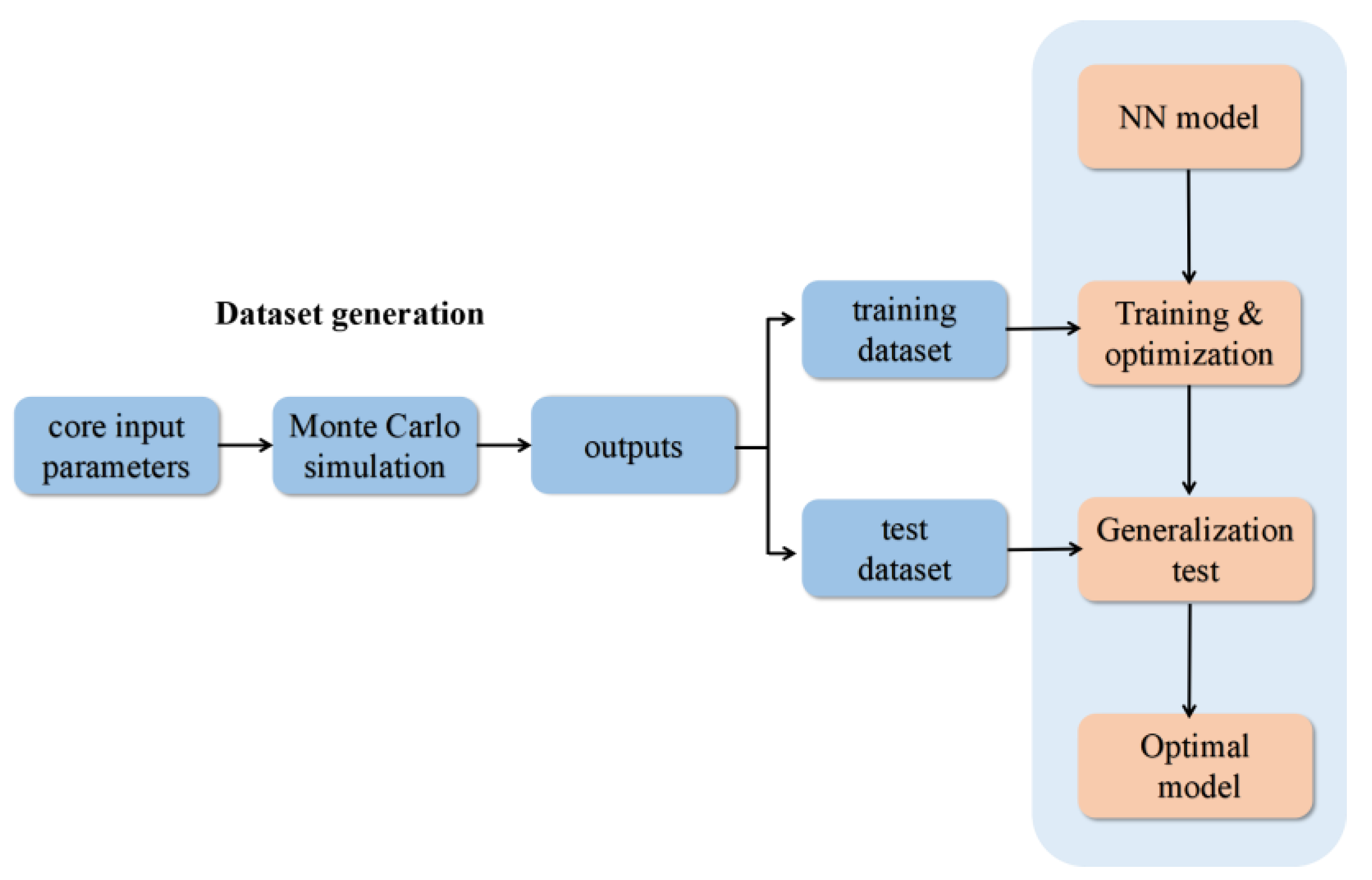
2.2. Dataset Generation

In order to train and optimize the surrogate model, firstly, the dataset is generated by modeling and simulating many operation states of the Molten Salt Reactor Experiment (MSRE) using the Monte Carlo code.

The MSRE is a type of liquid-fueled MSR that was designed and operated at Oak Ridge National Laboratory (ORNL) between 1965 and 1969 [24]. It is a 10 MW(t) reactor with the graphite moderator. Figure 6 presents the structure of the reactor core in MSRE.

The MSRE core is composed of a lattice of rectangular prism-shaped graphite “stringers” arranged vertically within a cylindrical reactor vessel. Each vertical graphite stringer has a side length of 5.08 cm and an axial length of 160.02 cm. Molten salt flows through more than 1000 channels [4]. Each channel is 1.016 cm thick and is formed by grooves in the side of the stringers, as presented in Figure 7. In the center of the core, four graphite stringers are left out to leave space for three control rod thimbles and an assembly consisting of three graphite sample baskets [26].

A high-fidelity geometry model of the MSRE core is built using the Monte Carlo code OpenMC [27,28], with the horizontal and vertical cross section of the reactor core described in Figure 8 and Figure 9. A detailed model of control rod and graphite sample assembly is also built, as shown in Figure 10. A summary of the main design parameters of the MSRE is presented in

Table 1. Main design parameters of the MSRE.

Main Materials
Fuel (mol%)	LiF-BeF2-ZrF4-UF4 (65-29.1-5-0.9)
Fuel salt density (g/cm3)	2.3275
Graphite density (g/cm3)	1.86
Inor-8 steel density (g/cm3)	8.77453
Hastelloy density (g/cm3)	8.86
Temperature for all materials (K)	911
Core main dimension
Inner core container radius (cm)	70.485
Outer core container radius (cm)	71.12
Inner reactor vessel radius (cm)	73.66
Outer reactor vessel radius (cm)	75.08875
Height of the up plenum (cm)	25.4
Height of the low plenum (cm)	25.4
Height of the vessel (cm)	236.474
Graphite stringer
Axial length of the graphite (cm)	160.02
Side length of the graphite (cm)	5.08
Fuel channel thickness (cm)	3.048
Fuel channel width (cm)	1.016

[25,26].

According to the input configuration of the neural network model, a total of 1500 dataset samples are generated by varying the nuclide concentration and control rod height within the core. The fuel compositions of the initial load and after shutdown in MSRE are obtained from the ORNL technical report [29]. A factor of 0.87 and 1.13 is applied, respectively, to the minimum and the maximum concentration in order to obtain a larger margin to cover the range for the intended application, which are summarized in

Table 2. The range of nuclide concentrations in MSRE.

Nuclide	Min/g	Max/g
U-234	676	887
U-235	70,900	74,700
U-236	337	1030
U-238	148	149
Pu-239	0	613
Pu-240	0	27.7
La-139	0	117
Ce-140	0	131
Pr-141	0	109
Ce-142	0	114
Nd-143	0	108

, and the control rod height is set to vary between 0 and 8 inches.

The neutron flux is tallied by dividing the mesh as follows. In the radial direction, each fuel channel is divided into a mesh cell, resulting in 1936 meshes (44 × 44); the mesh plot is shown in Figure 11. In the axial direction, the model is evenly divided into 10 layers, as shown in Figure 12, with the first and last layers representing the upper plenum and lower plenum, respectively, and the middle 8 layers representing the active region of the core.

Convergence analysis is necessary to obtain precise simulated results, and the Shannon entropy diagnostics is a commonly used tool to assess the source distribution convergence. Figure 13 shows the Shannon entropy versus batch curve, which indicates that 50 inactive batches are sufficient. Thus, the simulations are carried out using Monte Carlo code OpenMC with 150,000 particles per batch, 250 total batches, and 50 inactive batches. The outputs include the $k_{\mathrm{eff}}$ (1) and the neutron flux distribution of 10 layers (19,360). Each simulation produces a total of 19,361 neutronics outputs. A total of 1500 different reactor core states are generated through the stochastic sampling of nuclide concentrations and control rod height within the given range. A total of 1125 cases are used for training, and the remaining 375 cases are applied to test the applicability of the neural network.

2.3. Hyper-Parameters Optimization

Data preprocessing is carried out before training to ensure the model reliability. As shown in Table 2, the dataset containing several features is in different ranges. It is essential to normalize the dataset to reduce the impact of data dimensions on modeling and improve data integrity by reducing redundancy. The data is normalized using the Min-Max normalization, typically scaled to a target range of [0, 1]. The calculation formula is given in Equation (6):

$$x_{norm}=\frac{x-x_{min}}{x_{max}-x_{min}}$$

(6)

where, $x$ is the original data, $x_{min}$ and $x_{max}$ are the minimum and maximum values of the original data, respectively, and $x_{norm}$ is the normalized data.

Table 3. Hyper-parameters optimization range of NN.

Hyper-Parameters	Values Range
Number of hidden layers	[3–5]
Number of hidden neurons	[20–1936]
Activation function	[relu, sigmoid, tanh]
Optimizer	Adam
Learning rate	[0.1, 0.01, 0.001]

presents the optimization range of hyper-parameters considered in NN. Adam is selected as the optimizer based on preliminary experiments due to its faster convergence rates and better generalization ability than the traditional gradient descent algorithm [30]. Grid research is used to train and optimize the hyper-parameters, and the model is trained with 50 epochs.

3. Results

3.1. Surrogate Model Optimization

With the hyper-parameters selection range for the surrogate model provided in Table 3, the model has been repeatedly tuned and optimized. Figure 14 presents all the results of hyper-parameters optimization on 1125 cases, while Figure 15 presents the top 3 optimization results for each selected activation function. During the hyper-parameters optimization process, the learning rate is adjusted between 0.1, 0.01, and 0.001, the number of hidden layers is selected from 3 to 5, and the activation function is chosen from relu, sigmoid, and tanh where the network parameters are updated using the Adam optimizer. The figure indicates that when the learning rate was big, the gradient convergence rate is too fast to pass the extreme point and the surrogate model was underfitting. When the learning rate was small, the gradient convergence rate is too slow to reach the extreme point and the surrogate model may not capture the data characteristics well. For the relu activation function, the optimal learning rate is 0.01 and the number of neurons in hidden layer is about 20 to 120. For the sigmoid activation function, the optimal learning rate is 0.001 and the number of neurons in hidden layer is about 270 to 320. For the tanh activation function, the optimal learning rate is 0.01 and the number of neurons in hidden layer is about 20 to 220. The minimum target value was obtained using relu activation function.

The optimal structure of the surrogate model obtained is presented in

Table 4. The best combination of hyper-parameters.

Hyper- Parameters	Number of Hidden Layers	Optimizer	Learning Rate	Activation Function
values	4	Adam	0.01	relu

. The number of neurons in the hidden layer is related to the initialization of the network model, and thus the optimal network structure may vary for different applications. In the current study, optimal network structure for predicting the core parameters is a four-hidden layer network with 70 neurons, using an Adam optimizer with a learning rate of 0.01.

3.2. $k_{\mathit{eff}}$ Prediction

In this section, the test dataset is used to verify the generalization ability of the surrogate model in predicting $k_{\mathrm{eff}}$. The absolute error is typically used to quantify the difference, with the mathematical equation shown below.

$$absolute error=|{\widehat{y}}_i-y_i|$$

(7)

where, $y_i$ is the actual values of the sample i; and ${\widehat{y}}_i$ is the predicted values of the sample i.

Figure 16 compares the predicted and actual values of $k_{\mathrm{eff}}$ on the test dataset. It can be observed that the absolute error for most test samples falls within the 100 pcm interval, and very few test samples have an absolute error within the range of 100 pcm to 175 pcm. Figure 17 gives the histogram of the absolute error distribution for the $k_{\mathrm{eff}}$ prediction. Only 4.2% of the test samples have an absolute error outside the range of 100 pcm, while 95.8% of the samples have an absolute error within 100 pcm interval, demonstrating the strong predictive ability of the surrogate model.

3.3. 3D Neutron Flux Distribution Prediction

In this section, the test dataset is used to verify the generalization ability of the surrogate model in predicting neutron flux distribution. The relative error is used to quantify the deviation, with the min relative error (MinRE), mean relative error (MeanRE) and max relative error (MaxRE) represented by Equations (8)–(10), respectively.

$$MinRE=\underset{i=\mathrm{1,2}\dots n}{\min }\frac{\left|y_i-{\widehat{y}}_i\right|}{y_i}$$

(8)

$$MeanRE=\frac{1}{n}\sum _{i=1}^n\frac{\left|y_i-{\widehat{y}}_i\right|}{y_i}$$

(9)

$$MaxRE=\underset{i=\mathrm{1,2}\dots n}{\mathit{max}}\frac{\left|y_i-{\widehat{y}}_i\right|}{y_i}$$

(10)

where, n is the number of mesh cells; i is the mesh cell i; $y_i$ is the actual values of the mesh cell i; and ${\widehat{y}}_i$ is the predicted values of the mesh cell i.

The neutron flux distribution predicted using the surrogate model and calculated using the Monte Carlo code are compared on the test dataset. Considering the relative error between the predicted values using the surrogate model and the calculated values from OpenMC under each mesh cell, referring to analysis method from Chen [17], three representative instances are selected to evaluate the performance of the surrogate model. The selected instances are denoted as #1, #2, and #3, which represent the instance with the minimum max relative error, the instance with the maximum max relative error and a randomly selected instance where the relative error is calculated on each mesh cell, respectively. The comparison of the predicted and the actual neutron flux distributions for the three instances is presented in Figure 18a,b, Figure 19a,b and Figure 20a,b, respectively. The predicted neutron flux distribution exhibits a good agreement with the actual distribution. The neutron flux increases towards the center of the reactor core and decreases towards the periphery of the core. The highest neutron flux is observed in the center of the reactor core, which is consistent with the expected behavior of neutron flux in the reactor core.

The relative error distributions of each instance are shown in Figure 18c, Figure 19c and Figure 20c, respectively. The statistics of the relative errors in the three instances are presented in

Table 5. The statistics of the relative errors for the three instances.

		Error for Instance #1	Error for Instance #2	Error for Instance #3
full-core	MinRE	0%	0%	0%
	MeanRE	0.238%	0.319%	0.269%
	MaxRE	3.061%	6.639%	4.305%
edge region	MinRE	0%	0%	0%
	MeanRE	0.317%	0.334%	0.331%
activate region	MinRE	0%	0%	0%
	MeanRE	0.219%	0.315%	0.254%

. The figures show that the relative error is relatively small for the three instances, with most errors falling within the 1% range. Combined with the data in Table 5, the mean relative error for the first instance across the core is 0.238%, while the mean relative error for the second and three instances is 0.319% and 0.269%, respectively, which indicates that the predictive performance of the surrogate model is relatively reliable. While some mesh cells in the edge of the reactor core exhibit a significant relative error with values of 3.061%, 6.639%, and 4.305% for the first, second, and random instances, respectively. It is because the neutron flux calculated using the OpenMC code is of a very small order of magnitude compared to the activate region, leading to a relatively large relative error. Additionally, the prediction results of the surrogate model are influenced by the dataset, which also result in a high relative error at the edge region of the core. However, it only accounts for 1% of the core mesh. Overall, the error of the surrogate model, both in the active region and the edge region, is within the acceptable error range, which confirms the validity of the surrogate model.

The histograms in Figure 21, Figure 22 and Figure 23 provide the relative error distribution for the three representative instances, respectively. Most of the neutron flux, more than 99%, has a relative error within 2%, and indicate a high accuracy level in predictions of the surrogate model. The remaining 1% of the neutron flux has a relative error larger than 2%. As previously noted, it occurs mainly in the edge region of the core.

3.4. Computational Efficiency

The efficiency of the surrogate model and the Monte Carlo code is also evaluated. The simulations are performed on the personal computer with an AMD Ryzen 7 4800HS processor, manufactured by Advanced Micro Devices, Inc. (City of Santa Clara, CA, USA), clocked at 2.90 GHz, and a total of 8 cores. In addition, a GeForce RTX 2060 GPU manufactured by NVIDIA (City of Santa Clara, CA, USA) with 6 GB RAM is also utilized. According to the statistical analysis, it takes approximately 77 min to obtain the corresponding $k_{\mathrm{eff}}$ and channel-by-channel neutron flux for a steady-state critical neutron transport calculation using the OpenMC code. However, the optimal BPNN-based surrogate model takes only about one millisecond. The detailed computational time comparison between the Monte Carlo code and the surrogate model is presented in

Table 6. Time comparison for one steady-state transportation calculation.

	OpenMC Code	Optimal Surrogate Model
Computational time	77 min	0.002 s

. The significant improvement in calculation efficiency demonstrates the potential of the surrogate model in nuclear reactor analysis.

4. Conclusions

Accurate and rapid prediction of neutronics parameters in nuclear reactors plays an important role in the optimization of the design from both economic and safety perspectives. Although current high-fidelity neutron transport simulations provide precise solutions, the high computational cost poses a major challenge. Therefore, the present study focuses on developing an alternative method to provide accurate predictions in real-time.

In the current study, a novel three-dimensional surrogate model based on BP neural network has been proposed to reduce the computational cost associated with full-core neutron transport calculations, and its feasibility for predicting key neutronics parameters in the MSR is demonstrated. The input features include the concentrations of different nuclides, the height of the control rod and the axial information. The outputs consist of $k_{\mathrm{eff}}$ and channel-by-channel neutron flux distribution. The model is trained and optimized with the dataset generated using the Monte Carlo code OpenMC, and the generalization performance is evaluated with the test dataset. The numerical results show good agreement between the predicted and actual values. For $k_{\mathrm{eff}}$, most samples (95.8%) have an absolute error within 100 pcm. For neutron flux distribution, more than 99% of the neutron flux have a relative error within 2%. Additionally, the computational efficiency is also compared between the surrogate model and OpenMC code. Numerical results demonstrate that the surrogate model significantly improves the computational efficiency, with a speed-up of 2.31 million times compared to the OpenMC code.

The proposed surrogate model can predict three-dimensional key neutronics parameters accurately in real-time, which has important significance in improving the efficiency of the optimization design in a reactor core.

References

1. Serp, J.; Allibert, M.; Beneš, O.; Delpech, S.; Feynberg, O.; Ghetta, V.; Heuer, D.; Holcomb, D.; Ignatiev, V.; Kloosterman, J.L.; et al. The molten salt reactor (MSR) in generation IV: Overview and perspectives. Prog. Nucl. Energy 2014, 77, 308–319. [Google Scholar] [CrossRef]
2. Zuo, X.D.; Cheng, M.S.; Dai, Y.Q.; Yu, K.C.; Dai, Z.M. Flow field effect of delayed neutron precursors in liquid-fueled molten salt reactors. Nucl. Sci. Tech. 2022, 33, 96. [Google Scholar] [CrossRef]
3. Yu, K.; Cheng, M.; Zuo, X.; Dai, Z. Transmutation and Breeding Performance Analysis of Molten Chloride Salt Fast Reactor Using a Fuel Management Code with Nodal Expansion Method. Energies 2022, 15, 6299. [Google Scholar] [CrossRef]
4. Bostelmann, F.; Skutnik, S.E.; Walker, E.D.; Ilas, G.; Wieselquist, W.A. Modeling of the Molten Salt Reactor Experiment with SCALE. Nucl. Technol. 2022, 208, 603–624. [Google Scholar] [CrossRef]
5. Boyd, W.; Shaner, S.; Li, L.; Forget, B.; Smith, K. The OpenMOC method of characteristics neutral particle transport code. Ann. Nucl. Energy 2014, 68, 43–52. [Google Scholar] [CrossRef]
6. Dai, M.; Zhang, A.; Cheng, M. Improvement of the 3D MOC/DD neutron transport method with thin axial meshes. Ann. Nucl. Energy 2023, 185, 109731. [Google Scholar] [CrossRef]
7. Hansen, K.F.; Kang, C.M. Finite element methods in reactor physics analysis. Adv. Nucl. Sci. Technol. Acad. Press 1975, 8, 173–253. [Google Scholar]
8. LeCun, Y.; Bengio, Y.; Hinton, G. Deep learning. Nature 2015, 521, 436–444. [Google Scholar] [CrossRef]
9. Zhang, J.; Zhou, Y.; Zhang, Q.; Wang, X.; Zhao, Q. Surrogate Model of Predicting Eigenvalue and Power Distribution by Convolutional Neural Network. Front. Energy Res. 2022, 10, 919. [Google Scholar] [CrossRef]
10. Schlünz, E.B.; Bokov, P.M.; Van Vuuren, J.H. Application of artificial neural networks for predicting core parameters for the SAFARI-1 nuclear research reactor. In Proceedings of the 44th Annual Conference of the Operations Research Society of South Africa, Pecan Manor, Hartbeespoort, South Africa, 13–16 September 2015; pp. 12–22. [Google Scholar]
11. Jang, H.; Lee, H. Prediction of pressurized water reactor core design parameters using artificial neural network for loading pattern optimization. In Proceedings of the Transactions of the Korean Nuclear Society Virtual Spring Meeting, Online, 9–10 July 2020; pp. 9–10. [Google Scholar]
12. Chen, Y.; Wang, D.; Kai, C.; Pan, C.; Yu, Y.; Hou, M. Prediction of safety parameters of pressurized water reactor based on feature fusion neural network. Ann. Nucl. Energy 2021, 166, 108803. [Google Scholar] [CrossRef]
13. Mazrou, H. Performance improvement of artificial neural networks designed for safety key parameters prediction in nuclear research reactors. Nucl. Eng. Des. 2009, 239, 1901–1910. [Google Scholar] [CrossRef]
14. Zhang, Q.; Zhang, J.; Liang, L.; Li, Z.; Zhang, T. A deep learning based surrogate model for estimating the flux and power distribution solved by diffusion equation. EPJ Web Conf. 2021, 247, 8. [Google Scholar] [CrossRef]
15. Zhang, Q. A deep learning model for solving the eigenvalue of the diffusion problem of 2-D reactor core. In Proceedings of the Reactor Physics Asia 2019 (RPHA19) Conference, Osaka, Japan, 2–3 December 2019. [Google Scholar]
16. Wang, Z.; Huo, X.; Zhang, J.; Hu, Y. Geometry Optimization of Monte Carlo Model of Fast Reactor Core. At. Energy Sci. Technol. 2021, 55, 258. [Google Scholar]
17. Chen, S.; Ding, P.; Hu, S.; Xia, W.; Liu, M.; Yu, F.; Li, W. Optimization of Core Parameters Based on Artificial Neural Network Surrogate Model. In Proceedings of the International Conference on Nuclear Engineering, Shenzhen, China, 8–12 August 2022. [Google Scholar]
18. Cadenas, J.M.; Ortiz-Servin, J.J.; Pelta, D.A.; Montes-Tadeo, J.L.; Castillo, A.; Perusquía, R. Prediction of 3D nuclear reactor's operational parameters from 2D fuel lattice design information: A data mining approach. Prog. Nucl. Energy 2016, 91, 97–106. [Google Scholar] [CrossRef]
19. Cai, W.; Xia, H.; Yang, B. Research on 3D Power Reconstruction of Reactor Core Based on BP Neural Network. At. Energy Sci. Technol. 2018, 52, 2130. [Google Scholar]
20. Duderstadt, J.J.; Hamilton, L.J. Nuclear Reactor Analysis; Wiley: Hoboken, NJ, USA, 1976. [Google Scholar]
21. Oktavian, M.; Nistor, J.; Gruenwald, J.; Xu, Y. Preliminary development of machine learning-based error correction model for low-fidelity reactor physics simulation. Ann. Nucl. Energy 2023, 187, 109788. [Google Scholar] [CrossRef]
22. Ayodeji, A.; Amidu, M.A.; Olatubosun, S.A.; Addad, Y.; Ahmed, H. Deep learning for safety assessment of nuclear power reactors: Reliability, explainability, and research opportunities. Prog. Nucl. Energy 2022, 151, 104339. [Google Scholar] [CrossRef]
23. Li, J.; Cheng, J.; Shi, J.; Huang, F. Brief Introduction of Back Propagation (BP) Neural Network Algorithm and Its Improvement; Advances in Computer Science and Information Engineering; Springer: Berlin/Heidelberg, Gremany, 2012; Volume 2, pp. 553–558. [Google Scholar]
24. Haubenreich, P.N.; Engel, J.R. Experience with the Molten-Salt Reactor Experiment. Nucl. Appl. Technol. 1970, 8, 118–136. [Google Scholar] [CrossRef]
25. Robertson, R.C. MSRE Design and Operations Report Part I: Description of Reactor Design (ORNL-TM-728). Retrieved from US Department of Energy Office of Scientific and Technical Information. 1965. Available online: https://www.https://www.osti.gov/biblio/4654707 (accessed on 26 March 2023).
26. Fratoni, M.; Shen, D.; Ilas, G.; Powers, J. Molten Salt Reactor Experiment Benchmark Evaluation; University of California: Berkeley, CA, USA; Oak Ridge National Lab (ORNL): Oak Ridge, TN, USA, 2020. [Google Scholar]
27. Romano, P.K.; Horelik, N.E.; Herman, B.R.; Nelson, A.G.; Forget, B.; Smith, K. OpenMC: A state-of-the-art Monte Carlo code for research and development. Ann. Nucl. Energy 2015, 82, 90–97. [Google Scholar] [CrossRef]
28. Romano, P.K.; Forget, B. The Open MC Monte Carlo particle transport code. Ann. Nucl. Energy 2013, 51, 274–281. [Google Scholar] [CrossRef]
29. Bell, M.J. Calculated radioactivity of MSRE fuel salt. Oak Ridge Natl. Lab. 1970. [Google Scholar] [CrossRef]
30. Bei, X.; Cheng, M.; Zuo, X.; Yu, K.; Dai, Y. Surrogate models based on Back-propagation neural network for parameters prediction of the PWR core. In Proceedings of the 23rd Pacific Basin Nuclear Conference (PBNC), Chengdu, China, 1–4 November 2022. [Google Scholar]
Figure 1. The development framework of the surrogate model.
Energies 16 04044 g001
Figure 2. Typical BP neural network architecture.
Energies 16 04044 g002
Figure 3. A stacked method for 3D data representation.
Energies 16 04044 g003
Figure 4. Surrogate model architecture based on BP neural network.
Energies 16 04044 g004
Figure 5. Signal processing of the unit neuron element.
Energies 16 04044 g005
Figure 6. MSRE core vessel [25].
Energies 16 04044 g006
Figure 7. Dimensions and arrangement of the MSRE graphite stringers [26].
Energies 16 04044 g007
Figure 8. Horizontal cross section of the MSRE core at z = 80.00 cm.
Energies 16 04044 g008
Figure 9. Vertical cross section of the MSRE core at y = 0 cm.
Energies 16 04044 g009
Figure 10. Control rod and sample baskets of the MSRE.
Energies 16 04044 g010
Figure 11. All hyper-parameters optimization results.
Energies 16 04044 g011
Figure 12. The axial mesh plot in the core.
Energies 16 04044 g012
Figure 13. Shannon entropy versus.
Energies 16 04044 g013
Figure 14. All hyper-parameters optimization results.
Energies 16 04044 g014
Figure 15. Top 3 optimization results.
Energies 16 04044 g015
Figure 16. Comparison of the predicted value and the ground truth of k eff .
Energies 16 04044 g016
Figure 17. The absolute error distribution histogram of k eff .
Energies 16 04044 g017
Figure 18. The instance for the minimum relative error. (a) The predicted 3D channel-by-channel neutron flux distribution. (b) The true 3D channel-by-channel neutron flux distribution. (c) The relative error distribution.
Energies 16 04044 g018
Figure 19. The instance for the maximum relative error. (a) The predicted 3D channel-by-channel neutron flux distribution. (b) The true 3D channel-by-channel neutron flux distribution. (c) The relative error distribution.
Energies 16 04044 g019
Figure 20. The randomly selected instance. (a) The predicted 3D channel-by-channel neutron flux distribution. (b) The true 3D channel-by-channel neutron flux distribution. (c) The relative error distribution.
Energies 16 04044 g020
Figure 21. The relative error distribution histogram for the instance #1.
Energies 16 04044 g021
Figure 22. The relative error distribution histogram for the instance #2.
Energies 16 04044 g022
Figure 23. The relative error distribution histogram for the instance #3.
Energies 16 04044 g023