Roadmap to a Sustainable Energy System: Is Uncertainty a Major Barrier to Investments for Building Energy Retrofit Projects in Wide City Compartments?

Abstract

Along the roadmap to a Sustainable Real Estate-Scape, energy retrofit campaigns on wide city compartments represent a pivotal task, where the importance of the collaboration between the public and private sectors is crucial. Energy retrofit programs on building assets are subject to multiple uncertainty factors (e.g., climate, energy-economy forecasts, etc.) that act as a primary barrier to investment in this field. This paper aims to discuss risk management techniques to understand better how to deal with this kind of uncertainty. The research specifically addresses the techniques of sensitivity analysis and Monte Carlo simulation, focusing first on the phase of variables selection and their probability definition, including climatic, environmental, energy, economic, financial, and stochastic parameters. In this article, it is suggested to include correlation coefficients in the input variables of risk analysis, preferring the two-dimension Monte Carlo simulation to its simple version, since the results are more reliable when separating aleatory from epistemic uncertainty; thus, the results are more reliable. Moreover, it is seen how a sensitivity analysis based on percentile variations of the inputs provides a more accurate representation of risk if compared to the most common sensitivity analysis based on percentage deviations of the inputs. Conducting a sensitivity analysis using percentile variations gives realistic and reliable results, reflecting the tailored definition of uncertainty around the inputs on the basis of specific market analyses or historical series.

1. Introduction

The urban landscape is adapting to the new environmental, economic, social, energetic, and cultural challenges characterizing these times. As a result, many changes in perspective have (necessarily) redefined the relationship between States and markets, and between the public and private sectors, in the direction of a solid and smart collaboration to reach shared targets, where several and multifaced research fields have deepened this issue [1,2,3,4].

For what concerns energy sustainability, there have been many general directives at the European level due to the need to renovate entire urban areas in terms of energy efficiencyto tackle environmental threats that are less and less predictable and increasingly insidious. Among them there are, for instance, the “Energy Roadmap 2050” [5] as well as “The Clean Energy Package” [6], later discussed in this paper. In Italy, a recent important government initiative about energy efficiency in the building sector is the “110% Superbonus” [7]. Private stakeholders also dedicate manifold investments and projects to retrofitting their building assets and real estate holdings, intending to reduce the operating costs due to heating/cooling and to renovate the stocks. The best results (i.e., the optimal allocation of resources), however, may be achieved when the public and the private sectors strongly cooperate, for example, by providing financial incentives, and funding or tax allowances, since this approach allows for reducing and sharing the risks associated with such long-term investments [8,9,10,11].

Indeed, at a European level, significant energy sustainability results have already been achieved. For example, Eurostat data have confirmed that the 2020 targets for energy efficiency have been reached before the prearranged time limit [12]. Concerning clean energy policies, Europe is conducting a “Clean Energy Revolution” [13] based on common directives and shared targets; however, despite these significant achievements and milestones, our energy system is still to be transformed to become more sustainable in the long run, especially with regard to wide city compartments. The new task, therefore, is now to develop 2030–2050 strategies and to address both a shorter-term horizon, defining the following forthcoming measures to undertake, and a longer-term horizon, identifying future objectives, in the view of drawing the roadmap to a Sustainable Real Estate-Scape.

The big picture is outlined in the European strategy “Energy Roadmap 2050” [5], where different possible pathways for Europe are defined as explorative scenarios leading to a low-carbon economy. Here, the prearranged target is to reduce greenhouse gas emissions to 89–95% below 1990 levels by 2050 through clean energy European strategies.

Meanwhile, considering a shorter horizon, the European Commission presented a new set of measures establishing a stable legislative framework required to accomplish a clean energy transition before 2030, namely, The Clean Energy Package [6]. These clean energy measures are intended to make the European energy sector more stable, more competitive, and more sustainable, pivoting around three primary goals:

• putting energy efficiency first;
• achieving global leadership in renewable energies;
• providing a fair deal to consumers.

The package includes different legislative proposals covering energy performance in buildings, renewables, governance, and energy efficiency.

More significant investments from both the public sector and private stakeholders are fundamental, but so is access to capital and financial incentives. Energy efficiency schedules of large building stocks should be included in the broader panorama of economic activities, where financial incentives should be encouraged, contributing to “de-risk” energy efficiency investments. Naturally, given the long time-horizons of paybacks of energy retrofit projects, the risk is a pivotal issue.

There is uncertainty associated with energy efficiency results (e.g., profit, payback, and savings on consumptions), mainly since they rely on assumptions that are not certain (i.e., climate, energy consumption forecasts, and economic predictions).

As such, this paper will focus on the problem of leading building energy retrofit campaigns on wide building assets and city compartments, considering the importance of collaboration between the public and private sectors. This research contributes to the deep exploration of the sources of uncertainty in these kinds of analyses and the consequent risks reflected in the outcome.

In particular, this research will provide a practical case study to discuss how risk management techniques may help manage energy efficiency programs at a city level and discuss the issue: “Is uncertainty a major barrier to investments for building energy retrofit projects in wide city compartments?” The proposed risk-analysis technique may help a stakeholder identify the risk sources and “quantify” the risk connected to the investment.

Therefore, Section 2 will be dedicated to defining and deepening the concepts of risk and uncertainty. Section 3 will discuss the primary sources of uncertainty in energy retrofit projects, while Section 4 will introduce some risk management techniques. Section 5 will present the materials and methods for a practical case study. A cash-flow analysis will describe exemplary retrofit projects applied to a building asset in North Italy. Section 6 will allow for uncertainty in the cash-flow model, highlighting some critical issues. Section 7 will discuss the results achieved, and finally, Section 8 will draw the conclusions of the present work, introducing possible development of this research line.

2. Defining Risk and Uncertainty

Risk and uncertainty are sometimes improperly used as synonyms; however, the two concepts are different and should be used at different times of the valuation process. Several publications have discussed this issue, and generally, a unanimous distinction between the two concepts is defined as follows [14,15,16]:

• Uncertainty refers to the non-certain information used to build a forecasting model. It is caused by a lack of knowledge or imperfect information about a specific phenomenon/situation/condition/data [14]. As such, uncertainty represents anything that is unknown (i.e., uncertain, or not certain) about the parameters involved in the assessment model at the valuation date. Uncertainty should be considered from the analysis’s beginning since it affects a model’s inputs. A model’s data and inputs are based on only the best estimate of their values. In contrast, the actual future values may be different from the estimate due to unpredictable changes in, for instance, the economic, social, political or environmental conditions.
• Risk, instead, is a measure of how much the outcome of an assessment can vary because the uncertainty in the inputs is reflected in the output [14]. Risk, therefore, represents the possibility (i.e., the risk) that the output value will not turn out to be as previously estimated. According to these definitions, a possible range of outputs could be derived if a model’s input variables could be assessed as a probability distribution. This process of “propagation” of uncertainty from the inputs to the outputs allows for representing the risk of investment [17].

Regarding retrofit investments, uncertainty is related to the lack of perfect present and future knowledge of the input variables used in the energy-economy assessment models and approximations of the energy simulations that describe the physical phenomena. Several classifications of uncertainty have been proposed in order to categorize the different characteristics of risk while building energy analyses or during economic valuations [18]. When it comes to applying economic feasibility procedures to energy retrofit projects, all sources of uncertainty are mixed, bringing a high complexity to the forecasts. In the following paragraphs, a helpful classification of uncertainty sources is proposed to understand better an Author’s selection of the uncertain input variables presented in Section 6.1.3.

2.1. Model form Uncertainty and Parameter Uncertainty

An important distinction to clarify when discussing uncertainty is the difference between uncertainty in the model form and uncertainty in the parameters [19,20]. Model form uncertainty is also known in the related literature as model discrepancy, and it is caused by weaknesses in computer programs, numerical approximations, inaccuracies or missing physics [21]. Parameter uncertainty, instead, reflects the lack of knowledge in assessing input values inside the forecasting models [22].

2.2. Forward Uncertainty and Inverse Uncertainty

When it comes to applying uncertainty analyses to energy efficiency projects, another distinction should be introduced. As reported in [23], forward uncertainty quantification is on one side, and inverse uncertainty is on the other. Forward uncertainty is also called uncertainty propagation, and it is applied in building energy models by assessing uncertainty in the input variables of energy (-economy) forecasting models so as to quantify the uncertainty correspondingly in the outputs. In this case, the information flows forward from the input to the output. Inverse uncertainty analysis, otherwise called model calibration, follows the inverse information path because it is possible to determine unknown input variations through measured data (i.e., the output of an energy model) [24]. Forward and inverse uncertainty are related and can be integrated since inverse analyses require iterative forward simulations [25]. In contrast, inverse uncertainty results can be incorporated in forward simulations to forecast buildings’ energy results [26,27].

2.3. Aleatory Uncertainty and Epistemic Uncertainty

Another important distinction that helps enhance uncertainty analyses in energy retrofit investments regards the separation of aleatory uncertainty from epistemic uncertainty.

Intrinsic variability of the data investigated caused aleatory uncertainty. Aleatory uncertainty is also known as variability, stochastic, “type A” or irreducible. It is called irreducible since it represents a non-eliminable dispersion of values due to the heterogeneity of the observations. Considering the building energy retrofit sector, an example of aleatory uncertainty can be found in occupancy schedules and patterns.

On the other hand, epistemic uncertainty is simply caused by the lack of knowledge of specific data/phenomena used in the analysis. Epistemic uncertainty can be found in the literature as being “type B” uncertainty, state of knowledge, subjective and reducible. Reducible uncertainty assumes this name since it could be eliminated (theoretically) if more information were available at the time of the estimate [28,29]. In the energy retrofit field, epistemic uncertainty could be found, for instance, in estimating (future) energy prices.

3. Defining Sources of Uncertainty

As introduced in Section 2.1, parameter uncertainty refers to the uncertain assessment of the input parameters of a prediction model. In building energy analyses, this parameter uncertainty may regard the design parameters, inherent uncertain parameters, and scenario parameters. The following descriptions embrace the work presented in [18], and they are used to introduce and clarify the energy-economy uncertain inputs further discussed in Section 3.1 and Section 3.2.

Regarding uncertainty in design parameters, this is due to the different design stages during which feasibility analyses are iteratively produced. For example, the preliminary feasibility analyses cannot rely on specific assumptions at the early design stages. Construction materials, installations, and technologies are still to be defined, but this information will be better specified during the design refinement process. In the research, uncertainty in design parameters is suggested to be represented by continuous or discrete uniform distributions [30].

For inherent uncertain parameters, things are different since this information remains uncontrollable even at the final design stage. For instance, occupant behaviour or the difference between rated and actual plant system efficiencies cannot be foreseen. The authors in [30] suggest representing inherent uncertain parameters by normal distributions to catch the stochastic of the variables.

Finally, scenario parameters refer to potentially varying economic or climatic conditions. The uncertainty around these inputs may be derived from time-series analyses.

3.1. Energy Assessment: Uncertain Inputs

Multiple and non-predictable uncertainties are involved in energy retrofit projects. Energy consumption assessment depends on weather and climate, but these conditions are very difficult to predict in long-term analyses [31]. Energy requirements also depend on buildings’ construction properties, such as their envelope characteristics [31] or installation efficiency in situ [32], and this information can be very different during the building use if compared to the design forecasts. Stochastics are also associated with energy consumption concerning occupant behaviour [33], which only expresses a personal preference. Therefore, quantifying and describing uncertainty in the input parameters of building energy simulations is undoubtedly tricky, and the results may not be unanimous in the research [34].

Different research intensely discusses this argument, indicating a huge gap between the theoretical and actual energy performances during execution, operation and use [35]. This gap may be up to +34%, according to an analysis performed by [36] for non-domestic buildings.

A complete discussion of the building energy performance gap can be found in [37], where the authors discuss the significant causes of discrepancy between a predicted and actual energy consumption.

In 2002, research entitled “Quantifying the Effects of Uncertainty in Building Simulation”, developed by [38], identified three primary sources of uncertainty as being the thermo-physical properties of the building envelope, the casual and non-predictable heat gains, and the non-predicted infiltration rates. Again, in [39], the author of “Uncertainty in predictions of thermal comfort in buildings” pointed out the attention to several uncertain model parameters, such as the physical properties of materials, wind reduction factor, heat transfer coefficients, air temperature stratification, or radiant temperature of outdoor buildings, specifically deepening the uncertainty about indoor air temperature and wind pressure coefficients. Another very interesting research paper discussing several examples of parameter uncertainty quantification, including ground albedo, lighting and plug load and convective heat transfer coefficients, is entitled “Closing the building energy performance gap by improving our predictions” [19]. Again, ref. [20] developed uncertainty in terms of infiltration (i.e., air leakage area/distribution), workmanship issues at thermal bridges, occupancy variables (e.g., stochastic occupancy models), and HVAC (heating, ventilation and air conditioning) systems. Finally, a recent and very exhaustive review of uncertainty analysis in the energy assessment of buildings, performed by [23], identifies the primary sources of uncertainty in buildings analysis: weather data, building envelope properties, the HVAC system and occupant behaviour.

3.2. Economic Assessment: Uncertain Inputs

As it is for the energy assessment procedures, the economic valuations and forecasts are also subject to uncertainty. In fact, whatever technique is used to perform a feasibility (economic) analysis of a (energy retrofit) project, the outcome can only be considered the “best estimate” of the result. Each estimate is affected by uncertainties, such as uncertain information about the comparables, a lack of knowledge of the present and especially the future market conditions, or uncertain estimates of the input variables of the economic model.

Uncertainties are due to microeconomic factors and macroeconomic events; several financial [40] and economic [41] data are highly uncertain, affecting retrofit projects.

Economic and financial situations may undergo unforeseen and sudden changes, as has recently happened with the COVID-19 diffusion [42,43,44,45] and the outbreak of war in Ukraine [46,47]. Such events strongly impact economic/financial variables such as energy prices, the costs of construction or discount/growth rates.

Investment costs are very high, while possible returns on the investment are delayed in time, and this time-lag creates another source of uncertainty.

Different research deeply discusses this topic. For instance, a sensitivity analysis was applied to economic data by [48], who verified the reliability of the simulation results by varying the discount rate. Moreover, ref. [48] implemented a sensitivity analysis by varying the economical parameters of the discount rate, energy price and monetary values.

A paper by [49] applied a Monte Carlo simulation to identify the impact of changing energy prices on the net present value of an analysis. Additionally, ref. [50] used a Monte Carlo simulation when assessing the impact of discount rates with a simulation. Meanwhile, ref. [51] used all economic parameters, namely, the initial cost of retrofitting measures, the price of energy and the discount rate, to verify the critical inputs in a discounted cash flow analysis using a Monte Carlo simulation. Finally, ref. [52] simulated the variation of installation costs in zero-energy affordable houses. Through a sensitivity analysis, ref. [53] found that the energy prices and discount rates were the most critical economic variable in a cost-benefit analysis.

4. Risk Management Techniques

As introduced before, the outcome of any forecasting model, since it is for energy retrofit feasibility analyses, only represents the best estimate of the result. There is always the “risk” that the predicted outcome will differ from the future “actual” result.

The research has strongly encouraged the adoption of risk management techniques to enhance both energy and economic forecasting models. The authors of the present research have also discussed this issue in a comprehensive review of energy retrofits in building portfolios, pointing out the usefulness of integrating uncertainty management strategies in retrofit programs [54].

Risk management tools can generally be divided and categorized into three main groups, as fully explained in [55], i.e., deterministic, qualitative, and quantitative approaches. This categorization is also adopted and explained in [56].

Among the deterministic approaches, ref. [56] includes:

• Conservative benefit and cost estimating;
• Breakeven analysis;
• Risk-adjusted discount rate;
• Certainty equivalent technique;
• Sensitivity analysis;
• Variance and standard deviation;
• Net present value.

These approaches are punctual and give a general idea of the outcome. The most popular deterministic technique in the literature is undoubtedly the sensitivity analysis, belonging to the so-called one-factor-at-a-time technique [30] because one input variable (or a set of input variables) is varied, ceteris paribus, in order to understand how the output will respond to that change.

Among qualitative approaches, ref. [56] includes:

• Risk matrix;
• Risk registers coefficient of variation;
• Event tree (qualitative approach);
• SWOT analysis (strengths, weaknesses, opportunities, and threats);
• Risk scoring;
• Brainstorming sessions;
• Likelihood/consequence assessment.

These techniques are not able to “quantify” or “measure” the risk around the output of a forecasting model, but they can include qualitative aspects and non-measurable parameters. Due to their subjective nature, qualitative approaches are suitable in low-risk projects or at the early design stages, when the analyses should compare an investment’s pros and cons.

Finally, among the quantitative approaches, ref. [56] lists:

• Input estimates using a probability distribution;
• Mean-variance criterion;
• Decision tree analysis;
• Monte Carlo simulation;
• Analytical technique;
• Artificial intelligence;
• Fuzzy sets theory;
• Event tree (quantitative approach).

In contrast to qualitative approaches, quantitative techniques allow the measurement of uncertainty and variability of the result. The Monte Carlo simulation (MC) is very popular and helpful in supporting building energy efficiency projects because of its straightforwardness and versatility.

4.1. The Sensitivity Analysis for Energy Retrofits in Building Stocks

The use of a sensitivity analysis to enhance energy retrofit programs has been encouraged by the EU Commission Delegated Regulation 244/2012 [57] to identify and focus on the most critical factors that may affect the success of an investment. The approach is relatively straightforward but also very effective. A sensitivity analysis consists of varying one input parameter (or a predetermined set of parameters) in the forecasting model to record the consequent output variations. Each input variable is varied one-at-a-time, which allows for identifying the most impactful on the outcome. Usually, the inputs are varied as percentage or percentile deviations from their best estimate.

Several applications of this risk management technique can be found in the literature to improve the reliability of energy retrofit project forecasts. Both economic and energy inputs have been analysed to see how and to what extent their variation can impact the primary energy demand and the expected earnings, such as, for instance: climatic conditions, envelope thermal properties, usage schedule and utilisation hours [58], global/regional climate models [59], energy saving measures [60], building age, HVAC system and compactness ratio [61], and capital investment, operating costs and energy price [62], as well as energy price growth rates [63], discount rate [64] and the timeframe of the project [48].

4.2. The Monte Carlo Simulation for Energy Retrofits in Building Stocks

The Monte Carlo (MC) simulation is another popular way to include risk analysis in buildings’ energy efficiency projects [65]. Usually, an MC simulation is applied to the economic valuation of a retrofit plan. The MC analysis is an iterative procedure that produces multiple model output calculations by randomly changing the input variables among a predetermined range of possible values [16].

The first phase of an MC simulation consists, in fact, of the definition of a probability distribution of the input parameters contained in the forecasting model. The MC process, then, iteratively calculates the output value as the inputs change beneath their predefined range and probability. This allows us to describe the output as a single figure (i.e., the best estimate) and as a probability distribution, giving a more accurate understanding of the uncertainty related to the result.

Concerning Section 2.3, a more sophisticated approach to the MC simulation is the two-dimensional Monte Carlo (2DMC), which is an extension of the simple MC, where epistemic and aleatory uncertainty are distinguished and treated differently [28], giving a higher reliability and precision to the output [15].

The 2DMC has been applied in several and heterogeneous scientific sectors, such as biology [66], environmental science [67], medicine [68] and food science [69]. In contrast, implementing the 2DMC in energy efficiency projects and feasibility assessments is uncommon.

Even though the applications are still few in number, there are also some significant 2DMC applications in the field of energy retrofit of building assets, as reported in [70], to control the risk factors during an energy demand assessment, or as in [71], applied to an energy demand prediction model of building stock in Portugal, or [72], dedicated to a discussion of the uncertainty during the energy retrofit of a building asset in Italy.

5. Materials, Methods and a Pilot Case Study

In this research, an exemplary case study was selected to discuss uncertainty factors in retrofit projects and test the application of some risk management techniques, thus verifying how they may support valuation processes. The selected case study was a small asset of residential buildings in Bologna (Emilia Romagna, Northern Italy, as in Figure 1), constructed or renovated between 1950 and 1990. These buildings include traditional historical apartment blocks or recently constructed, multi-storey buildings. The professional studio “KG Progetti—Studio Progettazione Impianti” provided the data in Bologna (the data has been provided for research purposes only, and it is impossible, for the sake of owners’ privacy, to cite addresses, show photos of the buildings or provide additional information besides the one in this text). The Italian territory is divided into six climatic zones according to the conventional degree-day (DD) associated with the heating periods required, where zone A < 600 DD, 600 DD < zone B < 900 DD, 900 DD < zone C < 1400 DD, 1400 DD < zone D < 2100 DD, 2100 DD < zone E < 3000 DD, zone F > 3000 DD. The case study was in climatic zone E.

5.1. Energy Savings Due to Retrofit Actions

First, the buildings’ energy demand (Q) in the as-is state due to heating, domestic hot water, cooling and electricity were assessed through the software, Energy Plus.

In order to obtain the primary energy demand, or the yearly energy demand (YED), from the estimated Q, both the average seasonal global yields (η) and the primary energy conversion factors (fp) were considered as in Equation (1):

$$\mathrm{Y}\mathrm{E}\mathrm{D}=\frac{\mathrm{Q}\mathrm{*}\mathrm{f}\mathrm{p}}{\mathsf{\eta }}$$

(1)

In the equation above, η represents the ratio between the building energy demand (Q) and the actual energy required by the building’s installation to produce the necessary amount of energy [74].

Therefore, η takes into account the efficiency of the installations and systems in the building, including energy losses, and transforms the building energy demand (Q) into the delivered energy demand.

The primary energy conversion factor fp transforms the delivered energy demand into the primary energy demand on the basis of the different energy vectors involved in the systems supplied [75].

Finally, the YED is the actual amount of primary energy the building requires over the year for heating, cooling, hot water, and electricity.

After that, a set of energy retrofit actions was suggested to improve the energy performance of the buildings. The retrofit options considered are listed in

Table 1. Energy retrofit actions.

n.	Energy Retrofit Actions	Intervention Cost
1	Thermostatic valves	(90 € per valve)
2	Mechanical ventilation with heat recovery system	200 € per sqm
3	Condensing boiler with η > 1.06	cost function = [(25 * kWh) + 2600)] €
4	Air conditioners	90 € per sqm
5	Windows low-emissivity films	40 € per sqm
6	Windows with triple glazing and low emissivity coating	600 € per sqm
7	LED bulbs (100 lm/W)	30 € per bulb
8	Perlite thermalplaster, thickness = 3 cm, λ = 0.08 W/(m·K)	80 per sqm
9	Stone wool insulation, thickness = 8 cm, λ = 0.033 W/(m·K) or thickness = 16 cm, λ = 0.033 W/(m·K)	40 per sqm or 60 per sqm
10	Aerogel insulation, thickness=1 cm, λ = 0.015 W/(m·K)	140 € per sqm

, indicating the estimated intervention costs. The unitary costs were taken from regional price lists or specifically requested quotations. In addition, a cost function has been proposed for installing the condensing boiler since the cost estimate varies according to the required kWh. This cost function results from a linear regression analysis applied to the increase of costs according to the kWh of the boiler.

Table 2. Energy retrofit actions per building.

n. Energy Retrofit Action	Building A	Building B	Building C	Building D	Building E	Building F	Building G	Building H	Building I	Building L	Building M
1	x	x	x	x	x	x	x	-	x	x	x
2	-	-	-	-	-	-	-	x	-	-	-
3	x	x	x	x	x	x	x	x	x	x	x
4	x	-	-	-	-	-	-	-	-	-	-
5	x	-	x	x	x	-	x	-	x	x	-
6	-	x	-	-	-	x	x	x	-	-	x
7	x	x	x	x	x	x	x	-	x	x	x
8	-	-	-	-	-	-	-	-	-	-	-
9	x	x	x	x	x	x	x	-	x	x	x
10	-	-	-	-	-	-	-	x	-	-	-

illustrates the set of interventions selected to be implemented in each building.

The energy retrofit actions were implemented on the building asset, and the energy consumption post-retrofit was assessed via Energy Plus.

At this stage, it was possible to assess the energy savings produced by implementing the energy retrofit actions simply by comparing the pre- and post-retrofit YED. Equation (2) gives the amount of primary energy saved per year (kWh/y) due to heating/cooling, hot water and electricity (YED_saved), while the results are listed in

Table 3. Yearly energy demand saved.

	Total YED Pre-Retrofit (kWh)				Total YED Post-Retrofit (kWh)				YED Saved (kWh/y)
	Heating	Hot Water	Cooling	Electricity	Heating	Hot Water	Cooling	Electricity	Total
Building A	265,673	92,215	56,205	139,548	155,072	77,509	38,656	114,142	168,262
Building B	233,028	81,131	29,078	101,431	91,960	61,278	19,047	77,377	195,008
Building C	780,667	261,781	83,572	310,159	407,991	167,315	100,113	251,473	509,287
Building D	243,599	98,309	58,797	131,652	146,561	82,232	67,065	107,914	128,585
Building E	178,793	66,743	25,102	89,224	86,768	53,687	35,427	73,362	110,619
Building F	214,598	65,180	15,036	71,415	50,903	46,725	16,464	54,767	197,369
Building G	176,117	65,437	31,572	74,895	108,210	47,179	31,947	61,949	98,736
Building H	44,744	14,814	5,762	18,044	18,429	16,194	6,740	16,893	25,107
Building I	161,476	59,481	12,382	65,938	75,878	41,387	17,911	54,312	109,788
Building L	123,588	50,695	17,793	58,406	69,598	37,142	20,739	48,306	74,697
Building M	310,007	107,041	56,205	152,803	100,498	84,159	45,597	113,870	281,932

:

$$\begin{array}{c}{\mathrm{Y}\mathrm{E}\mathrm{D}}_{\mathrm{s}\mathrm{a}\mathrm{v}\mathrm{e}\mathrm{d}}=\left(\frac{\mathrm{Q}{\mathrm{h}\mathrm{e}\mathrm{a}\mathrm{t}\mathrm{i}\mathrm{n}\mathrm{g}}_{\mathrm{p}\mathrm{r}\mathrm{e}}}{{\mathsf{\eta }}_{\mathrm{h}\mathrm{e}\mathrm{a}\mathrm{t}\mathrm{i}\mathrm{n}\mathrm{g}{}_{\mathrm{p}\mathrm{r}\mathrm{e}}}}-\frac{\mathrm{Q}{\mathrm{h}\mathrm{e}\mathrm{a}\mathrm{t}\mathrm{i}\mathrm{n}\mathrm{g}}_{\mathrm{p}\mathrm{o}\mathrm{s}\mathrm{t}}}{{\mathsf{\eta }}_{\mathrm{h}\mathrm{e}\mathrm{a}\mathrm{t}\mathrm{i}\mathrm{n}\mathrm{g}{}_{\mathrm{p}\mathrm{o}\mathrm{s}\mathrm{t}}}}\right)\mathrm{*}\mathrm{f}{\mathrm{p}}_{\mathrm{h}\mathrm{e}\mathrm{a}\mathrm{t}\mathrm{i}\mathrm{n}\mathrm{g}}\\ \hspace{1em}\hspace{1em}\hspace{1em}\hspace{1em}\hspace{1em}\hspace{1em}+\left(\frac{{\mathrm{Q}\mathrm{c}\mathrm{o}\mathrm{o}\mathrm{l}\mathrm{i}\mathrm{n}\mathrm{g}}_{\mathrm{p}\mathrm{r}\mathrm{e}}}{{\mathsf{\eta }}_{\mathrm{c}\mathrm{o}\mathrm{o}\mathrm{l}\mathrm{i}\mathrm{n}\mathrm{g}{}_{\mathrm{p}\mathrm{r}\mathrm{e}}}}-\frac{{\mathrm{Q}\mathrm{c}\mathrm{o}\mathrm{o}\mathrm{l}\mathrm{i}\mathrm{n}\mathrm{g}}_{\mathrm{p}\mathrm{o}\mathrm{s}\mathrm{t}}}{{\mathsf{\eta }}_{\mathrm{c}\mathrm{o}\mathrm{o}\mathrm{l}\mathrm{i}\mathrm{n}\mathrm{g}{}_{\mathrm{p}\mathrm{o}\mathrm{s}\mathrm{t}}}}\right)\mathrm{*}\mathrm{f}{\mathrm{p}}_{\mathrm{c}\mathrm{o}\mathrm{o}\mathrm{l}\mathrm{i}\mathrm{n}\mathrm{g}}\\ \hspace{1em}\hspace{1em}\hspace{1em}\hspace{1em}\hspace{1em}\hspace{1em}+\left(\frac{\mathrm{Q}{\mathrm{h}\mathrm{o}\mathrm{t} \mathrm{w}\mathrm{a}\mathrm{t}\mathrm{e}\mathrm{r}}_{\mathrm{p}\mathrm{r}\mathrm{e}}}{{\mathsf{\eta }}_{\mathrm{h}\mathrm{o}\mathrm{t} \mathrm{w}\mathrm{a}\mathrm{t}\mathrm{e}\mathrm{r}{}_{\mathrm{p}\mathrm{r}\mathrm{e}}}}-\frac{\mathrm{Q}{\mathrm{h}\mathrm{o}\mathrm{t} \mathrm{w}\mathrm{a}\mathrm{t}\mathrm{e}\mathrm{r}}_{\mathrm{p}\mathrm{o}\mathrm{s}\mathrm{t}}}{{\mathsf{\eta }}_{\mathrm{h}\mathrm{o}\mathrm{t} \mathrm{w}\mathrm{a}\mathrm{t}\mathrm{e}\mathrm{r}{}_{\mathrm{p}\mathrm{o}\mathrm{s}\mathrm{t}}}}\right)\mathrm{*}\mathrm{f}{\mathrm{p}}_{\mathrm{h}\mathrm{o}\mathrm{t} \mathrm{w}\mathrm{a}\mathrm{t}\mathrm{e}\mathrm{r}}\\ \hspace{1em}\hspace{1em}\hspace{1em}\hspace{1em}\hspace{1em}\hspace{1em}+\left(\mathrm{Q}{\mathrm{e}\mathrm{l}\mathrm{e}\mathrm{c}\mathrm{t}\mathrm{r}\mathrm{i}\mathrm{c}\mathrm{i}\mathrm{t}\mathrm{y}}_{\mathrm{p}\mathrm{r}\mathrm{e}}-\mathrm{Q}{\mathrm{e}\mathrm{l}\mathrm{e}\mathrm{c}\mathrm{t}\mathrm{r}\mathrm{i}\mathrm{c}\mathrm{i}\mathrm{t}\mathrm{y}}_{\mathrm{p}\mathrm{o}\mathrm{s}\mathrm{t}}\right)\mathrm{*}\mathrm{f}{\mathrm{p}}_{\mathrm{e}\mathrm{l}\mathrm{e}\mathrm{c}\mathrm{t}\mathrm{r}\mathrm{i}\mathrm{c}\mathrm{i}\mathrm{t}\mathrm{y}}\end{array}$$

(2)

5.2. Monetary Savings through a Discounted Cash Flow Analysis

The overall economic evaluation of the profits derived from the retrofit actions applied to the asset was performed using a discounted cash flow analysis (DCFA) [76]. The DCFA makes it possible to verify the economic feasibility of the operation as a whole and to contextually assess the monetary benefit produced. For this analysis, the energy price for the gas distribution considered was 1.27 EUR/mc, while for electricity it was 0.36 EUR/kWh (source ARERA.it “Autorità di Regolazione per Energia Reti e Ambiente”).

The intervention costs and the monetary savings due to a lower YED were chronologically distributed along a timeline to determine the total cash inflows and outflows year by year.

In order to choose how to distribute the retrofit interventions on the buildings, a Gantt diagram was produced based on the cost-effectiveness of each investment. At the same time, the on-site construction time (t) was estimated by employing the hourly labour cost as in Equation (3). Finally, the cost-effectiveness of the retrofits was assessed by dividing the savings over the investment cost so that the higher the value, the more adequate the intervention, and therefore, the more convenient it is to apply it first:

$$\mathrm{t}=\frac{\mathrm{I}\mathrm{n}\mathrm{v}\mathrm{e}\mathrm{s}\mathrm{t}\mathrm{m}\mathrm{e}\mathrm{n}\mathrm{t} \mathrm{C}\mathrm{o}\mathrm{s}\mathrm{t}\mathrm{*}\mathrm{\%}\mathrm{L}\mathrm{a}\mathrm{b}\mathrm{o}\mathrm{u}\mathrm{r}}{\mathrm{H}\mathrm{o}\mathrm{u}\mathrm{r}\mathrm{l}\mathrm{y} \mathrm{L}\mathrm{a}\mathrm{b}\mathrm{o}\mathrm{u}\mathrm{r} \mathrm{C}\mathrm{o}\mathrm{s}\mathrm{t}\mathrm{*}8\mathrm{*} \mathrm{n}.\mathrm{w}\mathrm{o}\mathrm{r}\mathrm{k}\mathrm{e}\mathrm{r}\mathrm{s} \mathrm{*}\mathrm{w}\mathrm{o}\mathrm{r}\mathrm{k}\mathrm{i}\mathrm{n}\mathrm{g} \mathrm{d}\mathrm{a}\mathrm{y}\mathrm{s}}$$

(3)

In the formula above, %Labour is the percentage of the investment cost due to labour, 8 represents the work hours per day, n. workers is the number of on-site workers taken into account, while the yearly working days considered are 235.

Once the investments were chronologically defined, the DCFA could be performed, and the NPV was calculated according to the following formula in Equation (4). In the DCFA, the amounts are discounted to their present value using the discount rate (r) and algebraically added, which represents the net present value (NPV) of the cash flows [77]. The NPV defines whether and to what extent the savings produced by the investment are able to overcome the investment costs, verifying the feasibility and profitability of the retrofit operation:

$$\begin{array}{c}\mathrm{N}\mathrm{P}\mathrm{V}={\displaystyle \sum _{\mathrm{t}=0}^{\mathrm{T}}}(-\frac{{{\mathrm{I}\mathrm{n}\mathrm{v}\mathrm{e}\mathrm{s}\mathrm{t}\mathrm{m}\mathrm{e}\mathrm{n}\mathrm{t} \mathrm{C}\mathrm{o}\mathrm{s}\mathrm{t}}_{}}_{}}{{\left(1+\mathrm{r}\right)}^{\mathrm{t}}}+\frac{({\mathrm{F}\mathrm{i}\mathrm{n}\mathrm{a}\mathrm{n}\mathrm{c}\mathrm{i}\mathrm{a}\mathrm{l} \mathrm{S}\mathrm{u}\mathrm{b}\mathrm{s}\mathrm{i}\mathrm{d}\mathrm{e})\left[{(1+\mathrm{r})}^{10}-1\right]}_{}}{{\mathrm{r}(1+\mathrm{r})}^{10}}\\ \hspace{1em}\hspace{1em}\hspace{1em}\hspace{1em}\hspace{1em}\hspace{1em}+\frac{{{\mathrm{S}\mathrm{a}\mathrm{v}\mathrm{i}\mathrm{n}\mathrm{g}\mathrm{s}}_{\mathrm{g}\mathrm{a}\mathrm{s}}{\left(1+{\mathrm{g}}_{\mathrm{g}\mathrm{a}\mathrm{s}}\right)}^{\mathrm{t}}}_{}}{{\left(1+\mathrm{r}\right)}^{\mathrm{t}}}+\frac{{{\mathrm{S}\mathrm{a}\mathrm{v}\mathrm{i}\mathrm{n}\mathrm{g}\mathrm{s}}_{\mathrm{e}\mathrm{l}\mathrm{e}\mathrm{c}}{\left(1+{\mathrm{g}}_{\mathrm{e}\mathrm{l}\mathrm{e}\mathrm{c}}\right)}^{\mathrm{t}}}_{}}{{\left(1+\mathrm{r}\right)}^{\mathrm{t}}})\end{array}$$

(4)

In this equation, the investment cost is the total cost of the intervention, and the financial subsidies are a government incentive given as a 50% refund of the initial investment and granted back in ten years. Moreover, r represents the discount rate, while g is the growth rate of energy prices for the different energy vectors. The growth rates for gas and electricity are assessed by considering the time-series of the energy prices in the last 10 years, while the discount rate is estimated as the weighted average cost of capital (WACC) as reported in Equation (5):

$$\mathrm{W}\mathrm{A}\mathrm{C}\mathrm{C}=\frac{\mathrm{E}\mathrm{q}\mathrm{u}\mathrm{i}\mathrm{t}\mathrm{y}(\mathrm{r}\mathrm{i}\mathrm{s}\mathrm{k} \mathrm{f}\mathrm{r}\mathrm{e}\mathrm{e} \mathrm{r}\mathrm{a}\mathrm{t}\mathrm{e}+\sum \mathrm{r}\mathrm{i}\mathrm{s}\mathrm{k} \mathrm{p}\mathrm{r}\mathrm{e}\mathrm{m}\mathrm{i}\mathrm{u}\mathrm{m}\mathrm{s})}{(\mathrm{E}\mathrm{q}\mathrm{u}\mathrm{i}\mathrm{t}\mathrm{y}+\mathrm{D}\mathrm{e}\mathrm{b}\mathrm{t})}+\frac{\mathrm{D}\mathrm{e}\mathrm{b}\mathrm{t}\mathrm{*}(\mathrm{E}\mathrm{U}\mathrm{R}\mathrm{I}\mathrm{R}\mathrm{S}+\mathrm{B}\mathrm{a}\mathrm{n}\mathrm{k} \mathrm{S}\mathrm{p}\mathrm{r}\mathrm{e}\mathrm{a}\mathrm{d})}{(\mathrm{E}\mathrm{q}\mathrm{u}\mathrm{i}\mathrm{t}\mathrm{y}+\mathrm{D}\mathrm{e}\mathrm{b}\mathrm{t})}$$

(5)

In the equation above, the risk-free rate is a BTP10Y = 4.33%; the risk premiums are 3.00% (risk of construction and illiquidity); the EURIRS rate = 3.05%, where the EURIRS is the European interest rate swap; and the bank spread = 2.50%; Therefore, again, Equity = 50.00% of the investment cost, and, consequently, Debt = 50.00%, which produces a WACC = 6.44%.

Given that ggas = 1.96%, and gelec = 2.42%, the total initial costs of investment = 2,955,063 EUR, the total gas savings = 181,403 EUR, the total electricity savings = 42,894 EUR, with a financial subsidy of 50% and predefined time distribution of the intervention, and the NPV of the cash flows after a 15-year time span (T = 15) is 1,045,540 EUR. In comparison, after 30 years (T = 30) the NPV is 2,066,936 EUR, and the payback time is at year 10, as illustrated next in

Table 4. Yearly energy demand saved.

Time	Saving Gas	Saving Electricity	Financial Subside	Savings	Costs	Cash Flow	Discounted Cash Flow	NPV
Year	€	€	€	€	€	€	€	€
0	81,911	15,956	6,771	104,638	−135,425	−30,787	−30,787	−30,787
1	96,056	25,614	33,392	155,063	−532,418	−377,356	−354,524	−385,311
2	130,405	30,278	50,792	211,475	−348,002	−136,527	−120,506	−505,818
3	142,891	33,520	66,334	242,744	−310,837	−68,093	−56,466	−562,284
4	148,621	34,366	84,290	267,277	−359,109	−91,832	−71,544	−633,828
5	151,534	35,198	84,290	271,021	0	271,021	198,371	−435,457
6	175,421	38,890	120,431	334,742	−722,826	−388,084	−266,868	−702,324
7	207,804	50,709	147,753	406,266	−546,445	−140,179	−90,562	−792,887
8	211,877	51,936	147,753	411,566	0	411,566	249,805	−543,082
9	216,030	53,193	147,753	416,976	0	416,976	237,775	−305,307
10	220,264	54,480	140,982	415,726	0	415,726	222,720	−82,587
11	224,581	55,799	114,361	394,741	0	394,741	198,682	116,095
12	228,983	57,149	96,961	383,093	0	383,093	181,153	297,248
13	233,471	58,532	81,419	373,422	0	373,422	165,896	463,144
14	238,047	59,949	63,464	361,459	0	361,459	150,866	614,010
15	242,712	61,399	63,464	367,575	0	367,575	144,136	758,146
16	247,470	62,885	27,322	337,677	0	337,677	124,401	882,547
17	252,320	64,407	0	316,727	0	316,727	109,623	992,170
18	257,266	65,966	0	323,231	0	323,231	105,106	1,097,275
19	262,308	67,562	0	329,870	0	329,870	100,774	1,198,050
20	267,449	69,197	0	336,646	0	336,646	96,622	1,294,672
21	272,691	70,872	0	343,563	0	343,563	92,641	1,387,313
22	278,036	72,587	0	350,623	0	350,623	88,824	1,476,138
23	283,485	74,343	0	357,829	0	357,829	85,165	1,561,303
24	289,042	76,142	0	365,184	0	365,184	81,657	1,642,960
25	294,707	77,985	0	372,692	0	372,692	78,294	1,721,254
26	300,483	79,872	0	380,355	0	380,355	75,069	1,796,324
27	306,373	81,805	0	388,178	0	388,178	71,978	1,868,302
28	312,378	83,785	0	396,162	0	396,162	69,014	1,937,315
29	318,500	85,812	0	404,313	0	404,313	66,172	2,003,488
30	324,743	87,889	0	412,632	0	412,632	63,448	2,066,936

.

6. Dealing with Uncertainty

The DCFA conducted in Section 5.2 produced the best estimate of the NPV of the cash flows due to the energy retrofit measures applied to the building asset. The NPV assessment, however, depends on a plethora of variables that may differ from the figures predicted by the valuer (in this case, the authors of the paper) to the best of the knowledge available at the time of the estimate. In reality, multiple factors may differ from the estimate or be affected by other events not considered in the predictions.

Therefore, to produce a complete assessment of the NPV, uncertainty was incorporated in the model using an MC simulation.

First thing, the uncertain parameters of the NPV must be defined. According to Equation (4), the NPV assessment is a function of the following inputs: investment cost, financial subside, the discount rate “r”, the time T, the gas and electricity savings, as well as the growth rates of the gas and electricity prices. The discount rate, in turn, depends on the equity and the debt ratio, the risk-free rate, the EURIRS rate and the bank spread, as in Equation (5).

These were then considered the uncertain factors in the DCFA model, ceteris paribus.

Each input was assigned a probability distribution, as represented in

Table 5. Definition of probability distributions in uncertain parameters.

Input Variables	Best Estimate	Distribution	Minimum	Maximum
Gas Savings	188,777 €	triangular	169,899 €	207,654 €
Electricity Savings	42,755 €	triangular	38,480 €	47,031 €
Gas growth rate	1.96%	normal	0.00%	9.49%
Electricity growth rate	2.42%	normal	0.00%	7.28%
Debt	50.00%	rectangular	35.00%	60.00%
BTP (10Y)	4.33%	normal	0.16%	6.74%
EURIRS	3.05%	normal	−0.08%	3.48%
Bank Spread	2.50%	rectangular	0.50%	4.50%
Financial Subside	50.00%	rectangular	50.00%	65.00%
Time	0.00 year	rectangular	0.00 year	3.00 years
Investment Cost	2,955,063 €	triangular	2,659,557 €	3,250,569 €

, that could capture the variability of that parameter.

The probability distributions used in this research were triangular [41], normal [78] or rectangular [79]. The distributions and the minimum and maximum values considered resulted from specific market analyses, historical series analyses or literature reviews.

6.1. The MC Simulation

6.1.1. The Simple MC Simulation

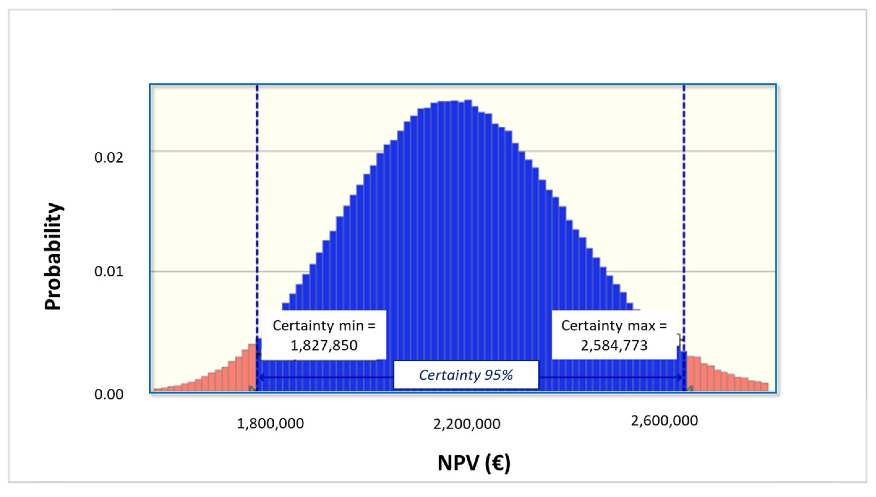
The first MC simulation conducted was a simple MC analysis: the simulation trials were 1,000,000 and were performed with the Crystal Ball software. The trials iteratively re-calculated the NPV forecast by randomly changing the inputs of the DCFA model among their corresponding predefined probability distribution. The results are shown in Figure 2.

The value predicted by the MC simulation as the average of the 1,000,000 NPVs simulated was 2,189,904 EUR, which was slightly different from the discrete use of the DCFA model. The standard deviation was 213,295, representing the uncertainty associated with the feasibility analysis. The skewness index was 0.16 and indicates the degree of symmetry of the distribution around the mean. The distribution was similar to the normal distribution but had no significative tails extending towards positive/negative values.

6.1.2. The Simple MC Simulation with Correlations among the Input Values

A second MC simulation was performed after Pearson correlation coefficients among the input variables were defined. This way, the iterative NPV calculation respected the correlations among the input parameters so that a coefficient equal to +1 represented a perfectly positive correlation, a perfectly negative correlation had a coefficient of −1, while if two variables were independent, their Pearson correlation coefficient was 0.

The coefficients assigned in the matrix in Figure 3 have been defined through the pairwise analysis of the time-series of the data used in the DCFA, collected from 2013 to 2023 every trimester. The results, as shown in Figure 4, produced an average value of the iterations equal to 2,189,550 EUR, with a standard deviation of 194,310, and a skewness of 0.177.

6.1.3. The 2DMC Simulation

The third MC analysis conducted in this research was a two-dimension simulation, where the risk factors in the model were treated differently if they were subject to variability or uncertainty. As introduced in Section 2.3, a parameter was subject to variability when it described a “varying” population. It could naturally take on different values due to the same nature of the considered variable. Conversely, a parameter was subject to uncertainty if it was impossible to determine a specific value only because of insufficient or incomplete information.

Since a 2DMC separates the concepts of uncertainty and variability, the risk simulation has a greater accuracy. In a 2DMC simulation, uncertain inputs are sampled separately from variable parameters, and two iteration loops occur. An inner loop simulates the variability, while uncertainty is simulated in the outer loop.

The outer simulation acts like it could, theoretically, “eliminate” the uncertainty due to a lack of information by iterating the simulations of the uncertain variables first. At that point, the values of the uncertain variables are frozen under the assumption that uncertainty has, thus, been eliminated (because the parameters have been determined), and the “variable” inputs (irreducible uncertainty) are then randomized in the second simulation loop since their variability cannot be eliminated by more hypothetical knowledge.

In this simulation, the outer loop was performed by the variables: electricity and gas savings, the growth rates, the BTP and EURIRS rate, and the bank spread.

The inner loop randomized the parameters: debt, time, investment cost, and financial subside.

Throughout, 1000 iterations were performed for the outer loop (uncertainty) and 1000 iterations for the inner loop (variability), leading to running the simulation 1,000,000 times. The results are illustrated in

Table 6. 2DMC results.

	MC (without Correlations)	MC (with Correlations)	2DMC (with Correlations)
Trials (n.)	1,000,000	1,000,000	1000*1000
Mean (€)	2,189,904	2,189,550	2,193,980
Median	2,183,849	2,183,722	2,192,265
Standard Deviation (€)	213,295	194,310	121,731
Skewness	0.160	0.177	0.123
Kurtosis	2.967	2.916	2.674
Coeff. of Variability	0.097	0.089	0.056
Minimum (€)	1,287,791	1,403,740	1,896,921
Maximum (€)	3,403,721	3,147,808	2,533,225
Range Width (€)	2,115,930	1,744,068	636,304

, compared to the previous simulations.

The mean value for the NPV simulations was quite similar in the three MC versions, but the standard deviation was reduced, and in the 2DMC it was 121,731; therefore, lower than the corresponding value in the 1D simulation.

Moreover, in the 2DMC simulation, the range width (maximum value–minimum value) was smaller if compared to other simulations; therefore, at the same level of certainty, the 2DMC model produced a more robust range of results.

7. Results

Sensitivity Analysis

A sensitivity analysis was performed for the conclusion of this paper on the output of the DCFA, showing changes in the NPV due to percentile variations/percentage deviations in the input values of the model. As each input was varied one-at-a-time (and not all simultaneously as in the MC simulation), it will become clear which factors impacted the NPV most [80]. This is important because the most influential factors must be carefully monitored throughout the retrofit operation.

In this research, the authors compared the most popular sensitivity analysis based on percentage deviations of the inputs, in

Table 7. Sensitivity analysis with percentage deviations of the inputs.

	Input Percentage Deviations			Output Variation
Variable	Downside	Upside	Base Case	Downside (−10%)	−5.0%	0.0%	5.0%	Upside (10%)	Range
Gas Savings (€)	163,263	199,543	181,403	2,002,156	2,139,645	2,277,133	2,414,622	2,552,110	549,954
Investment Cost (€)	2,659,557	3,250,569	2,955,063	2,393,942	2,335,538	2,277,133	2,218,729	2,160,325	233,617
Financial Subside (%)	59%	72%	65%	2,160,900	2,219,017	2,277,133	2,335,250	2,393,367	232,467
BTP (10Y) (%)	3.897%	4.763%	4.330%	2,370,274	2,323,230	2,277,133	2,231,963	2,187,697	182,577
Electricity Savings (€)	38,604	47,183	42,894	2,207,589	2,242,361	2,277,133	2,311,906	2,346,678	139,090
EURIRS (%)	2.745%	3.355%	3.050%	2,342,345	2,309,506	2,277,133	2,245,221	2,213,760	128,585
Gas growth rate (%)	1.62%	1.98%	1.80%	2,215,840	2,246,255	2,277,133	2,308,483	2,340,313	124,472
Bank Spread (%)	2.250%	2.750%	2.500%	2,330,447	2,303,634	2,277,133	2,250,942	2,225,055	105,392
Debt (%)	45%	55%	50%	2,239,929	2,258,454	2,277,133	2,295,970	2,314,964	75,035
Electricity growth rate (%)	2.16%	2.64%	2.40%	2,255,848	2,266,382	2,277,133	2,288,108	2,299,312	43,463
Time (year)	0	0	0	2,277,133	2,277,133	2,277,133	2,277,133	2,277,133	0

, versus the percentile variations, in

Table 8. Sensitivity analysis with percentile variations of the inputs.

	Input Percentile Variations			Output Variation
Variable	Minimum	Maximum	Base Case	Minimum	Maximum	Range
Gas Savings (€)	178,341	199,212	181,403	2,230,722	2,547,086	316,364
BTP (10Y) (%)	4.885%	3.775%	4.330%	2,163,162	2,397,191	234,029
Financial Subside (%)	52%	64%	65%	2,035,726	2,250,310	214,584
Gas growth rate (%)	1.71%	2.21%	1.80%	2,246,255	2,424,899	178,644
Time (year)	2.7	0.6	0	2,065,158	2,238,197	173,039
Debt (%)	38%	58%	50%	2,185,270	2,334,118	148,848
EURIRS (%)	3.339%	2.645%	3.050%	2,216,962	2,364,152	147,190
Investment Cost (€)	3,118,415	2,791,711	2,955,063	2,212,563	2,341,704	129,140
Bank Spread (%)	2.700%	2.300%	2.500%	2,235,373	2,319,684	84,310
Electricity Savings (€)	40,392	45,119	42,894	2,236,570	2,313,209	76,639
Electricity growth rate (%)	2.11%	2.73%	2.40%	2,251,240	2,307,491	56,251

.

The percentage deviations-sensitivity analysis showed an upside and downside variation of the inputs by varying a percentage of ±10% of the base value of the inputs.

The percentile variations-sensitivity analysis was set between the 10th and 90th percentile of the inputs, where the percentiles of the variables were determined using the identical probability distributions as those already illustrated in Table 5 for the MC simulations. In this case, the tenth percentile represented the downside, while the ninetieth was the upside case. Consequently, the changes in NPV corresponding to each change in the input variables can be summarised, as in Table 7 and Table 8 and in the tornado diagrams in Figure 5 and Figure 6, which show graphically the factors whose uncertainty produced the more significant impact on the results. This gives a clear understanding of which factors are the most important for ensuring the feasibility of an intervention. The interpretation of the graphs is simple: the longer bars represent the inputs that have the most significant impact on NPV, and the shorter ones influence it the least. The results were placed into comparison, showing the differences between the two approaches and pointing out the strengths and weaknesses. For example, it represents how a best-estimate null value (time t = 0) has a null variation in a sensitivity analysis with percentage deviations but an important impact on the output in the sensitivity analysis with percentile variations.

In the authors’ opinion, the sensitivity analysis based on percentile variations of the inputs is a more accurate representation of risk if compared to the percentage deviations.

Both sensitivity analyses identify the gas savings as the major impactful variable on the outcome, and the financial subsidy is also recognised as one of the inputs with the most impactful influence on the NPV.

However, the authors feel that the percentile variations-sensitivity analysis can be considered as a more reliable approach for, basically, two major reasons:

• First, the percentage deviation sensitivity analysis only varies the inputs of a predetermined percentage, in this case ± 10% of the best estimate, without further specific considerations. In contrast, the percentile variations are based on a tailored definition of the input’s probability distributions and ranges based on historical series analyses, specific forecasts or market analyses.
• Second, only the percentile variation-sensitivity analysis is able to capture the impact of time variations on the DCFA results, while the percentage deviation-sensitivity analysis also tends to overestimate the impact of the investment costs on the outcome. This is because applying a percentage on a quantity, in some cases, may be quite misleading. A variable whose best estimate is 0 will not be varied at all (as in the case of time t), while a large number will be varied too much (as it is for the investment cost).

8. Discussion and Conclusions

In the field of energy sustainability, the object of this research was the discussion of sources of uncertainty and risk management techniques within the roadmap to the transition to a Sustainable Real Estate-Scape.

The analysis regarded the energy efficiency project of a building asset in North Italy, under the perspective of facing unpredictable and insidious environmental threats in the coming years. Therefore, the core of this study was the discussion and comparison of risk analysis techniques applied to building energy efficiency projects, focussing on the Monte Carlo simulation and sensitivity analyses, arguing the prominence of some crucial issues that have been too often overlooked or neglected in the specific literature, such as the identification of main uncertainty sources, the consequent input selection and definition, the discussion of the most appropriate risk analysis technique, and introducing details and precautions that could improve the reliability of the results.

Specifically, the scope of the study was to compare the results of a sensitivity analysis and a Monte Carlo simulation in some different variants: the sensitivity analysis was applied in two versions, i.e., as percentile variations or percentage deviations of the input variables, whereas the Monte Carlo simulation was applied in its simple and two-dimension versions, while also experimenting the difference between defining and not defining correlation coefficients among the input variables.

The first contribution of this research is the discussion and reasoning about the delicate process of variables selection and their statistical modelling, which should realistically reflect every source of uncertainty, including climatic, energy, economic, financial, and stochastic variables. Tailored market analyses and historical series helped the definition of the probability distributions.

The second contribution of the present paper regards recognising the importance of defining correlation coefficients among the input variables.

Additionally, the use of a two-dimensional Monte Carlo simulation was tested on the case study, and it was revealed to be a better technique for risk simulation since it allows for separating the epistemic from aleatory uncertainty, leading to more accurate results.

Finally, another contribution of this research is using sensitivity analysis to identify the significant risk factors and to compare different ways of performing it. There are, in fact, considerable differences in the results if a sensitivity analysis is performed considering percentage deviations of the variables or percentile variations of the variables. Consequently, a percentile variations-sensitivity analysis can be considered a more reliable approach.

In conclusion, the risk-simulation methodologies, developed to answer several critical questions, have been tested on an interesting case study concerning the energy efficiency of a small building portfolio in North Italy.

The results are rather significant, as they provide an innovative discussion of risk simulations in a building energy retrofit. It is demonstrated how it is essential to include risk analyses in energy retrofit studies to identify and “quantify” the primary risk sources and, therefore, to try to overcome the uncertainty problem as a significant barrier to investment.

In further developments of this research line, the authors wish to experiment with the results of a Monte Carlo simulation in other variations besides the two-dimension version, such as for instance, the Monte Carlo Markow chain, and to verify if, and to what extent, these kinds of more specific techniques may help to deal with risk management.