An Investigation of Tourism, Economic Growth, CO₂ Emissions, Trade Openness and Energy Intensity Index Nexus: Evidence for the European Union

Abstract

Tourism has become one of the most important sectors in many countries, significantly contributing to their economic growth and development. However, the expansion of tourism has also brought about various environmental and social challenges. The relationship between tourism, economic growth, trade openness, and the environment is diverse and complex. The objective of this paper is to investigate the relationship between the international tourism development index, GDP per capita, CO₂ emissions, trade openness index as well as the energy intensity index in EU 27, over the 1995–2019 period. A composite index for international tourism was developed using the Principal Component Analysis (PCA). Panel Autoregressive distributed lag (ARDL) approach is used to reveal the long- and short-run impact of GDP per capita, CO₂ emissions, trade openness index as well as the energy intensity index on the tourism development index. Panel ARDL estimates confirm some of our research hypotheses: at the level of EU countries, there is a short-run relationship between tourism and GDP per capita, but only in a few EU countries, trade openness influences tourism development index. Dumitrescu-Hurlin causality test confirms long-run feedback relationship between tourism development index and trade openness, between tourism development index and CO₂ emissions, and between tourism development index and GDP and unilateral causality running from tourism development index towards energy efficiency.

1. Introduction

Tourism plays a significant role in the economic growth of European Union countries. According to the European Travel Commission, the travel and tourism sector in the EU accounted for 9.9% of the total EU Gross Domestic Product (GDP) in 2019 and generated around 27 million jobs in the region [1]. During the pandemic, European Travel Commission reports showed a 62% drop in tourist arrivals in Europe in 2021 compared to 2019 [1]. However, the outlook for tourism recovery in the coming years remains positive, so domestic travel is expected to surpass pre-pandemic peaks in 2022, while international travel will surpass pre-pandemic peaks in 2024 at the earliest. Tourism creates direct and indirect economic benefits. Direct benefits include employment opportunities in the tourism sector, foreign exchange earnings from international tourists and tax revenues [2,3] resulting from tourism activities. Indirect benefits include growth in other sectors such as transport, hospitality, and retail, which support the tourism industry. Moreover, tourism stimulates investment in infrastructure development such as airports, roads, and hotels, which create jobs and supports the country’s economic growth [4,5]. It is worth noting that the impact of tourism on economic growth can vary depending on the type of tourism and the destination. As a consequence, the environment and local communities are affected by mass tourism, and the benefits of tourism may not always be distributed evenly across regions and social groups. In Europe, the tourism sector generates significant revenue and employment opportunities, contributing to overall economic growth. For instance, countries like France, Spain, and Italy heavily rely on international tourism to drive their economies. Therefore, although tourism can contribute positively to economic growth in EU countries, it is important to manage tourism in a sustainable manner, considering environmental, social, and cultural factors to ensure long-run benefits for both tourists and for host communities.

Tourism and the environment share a bidirectional relationship, as has been observed in literature review. This relationship is complex, as the environment provides many attractions for tourists, while tourism providers change the environment to build hotels, restaurants, and other facilities. At a macro level, tourism is also linked to climate change, which poses a risk to tourist attractions and has a direct impact through CO₂ emissions [6,7]. The effects of climate change include melting snow, rising sea levels, and natural disasters. Thus, climate changes affect to some extent, both the behavior and the attitude of tourists [8]. Tourism activities can impact the environment through carbon emissions, resource consumption, and waste generation. European countries, such as Iceland [1] and Switzerland, have embraced sustainable tourism practices by promoting eco-friendly accommodations, encouraging responsible tourist behavior, and investing in renewable energy sources to mitigate environmental impacts.

Tourism has become, over time, one of the significant economic sectors in many countries. However, the increase in this sector leads to several important challenges for both the environmental and social aspects. Therefore, trade openness, as a crucial component of economic growth, proved to have a significant impact on the tourism sector. For example, trade openness can increase the competitiveness of the tourism sector, thus contributing to economic growth. In addition, trade openness can lead to negative environmental impacts, such as increased energy consumption, pollution, and exploitation of natural resources [9]. Thus, the impact of trade openness on tourism has direct and indirect effects that can be positive or negative based on the level of development of the country concerned.

Therefore, it is important for policy makers to consider the trade-offs between tourism development, economic growth, trade openness, and environmental sustainability when formulating policies and strategies for the tourism sector.

The objective of our paper is to investigate the short- and long-run nexus between the international tourism development index, economic growth, CO₂ emissions, trade openness index as well as the energy intensity in EU27. In order to better evaluate tourism, we will build a comprehensive index based on three variables: international tourism receipts, international tourism arrivals, and international tourism expenditures. For this purpose, we will use the PCA technique and an ARLD model based on panel data. This approach has the advantage that is allows both time and spatial dimension in the analysis, which increases the number of observations and increases the degrees of freedom and reduces the chances of multicollinearity.

Our investigation seeks to contribute to literature both from theoretical as well as empirical point of view. First, the survey of the relevant papers allowed us to assess the relationship between the selected variables. Second, the empirical analysis based on dynamic models and panel data enables the investigation of short- and long-run effects of determinants over the endogenous variable—the international tourism development index. Third, the analysis reveals some policy implications and further research directions to be followed in the future.

The rest of our paper is organized as follows. Section 2 reviews the relevant literature on the correlation between tourism, economic growth, CO₂ emissions, environment, and trade openness. Section 3 presents statistical data and methodology; Section 4 is dedicated to the empirical analysis. Section 5 presents detailed discussions, policy implications, and limitations of our paper. The research ends with the concluding remarks.

2. Literature Review

2.1. Tourism and Economic Growth

The correlation between tourism and economic growth has been approached in the literature both from the perspective of the Keynesian theory of the multiplier, and from the perspective of the theory of endogenous growth when it is applied to the tourism sector. Among the first works dedicated to this subject are those of Lanza and Pigliaru [10,11] who found that the countries that were highly specialized in tourism were small countries and the work of Balaguer and Cantavella-Jorda [12] who analyzed for the first time the tourism-led growth hypothesis. Regarding the indicators for measuring economic growth and those of tourism, in a relatively large number of articles, economic growth is analyzed using indicators such as GDP per capita, % change GDP, real GDP, as well as industrial production [13], Human development Index [14], while the number of tourist arrivals, together with international tourist receipts, are the terms utilized in analyzing tourism expansion. However, there is still controversy over the indicators used or their practical significance. After a thorough analysis of the empirical literature regarding the causality between tourism and economic growth, we have identified four hypotheses: tourism-led growth hypothesis, growth-led tourism hypothesis, bidirectional causality hypothesis, or no causality hypothesis [12].

The hypothesis according to which tourism is significant for driving economic growth has remained one of the most supported in the literature. To analyze the influence of tourism on economic growth, a series of various models and techniques were applied: time series, panel data, and cross-sectional data. Balaguer and Cantavella-Jorda [12] conducted the first empirical work on the tourism-led growth hypothesis (TLGH). Beginning with this study, a relatively large number of papers were published, including case studies, methodologies, and databases. Balaguer and Cantavella-Jordà [12] analyzed the impact of tourism on growth starting from three variables: international tourism revenues, real GDP, and the real effective exchange rate in Spain for the time frame 1975–1997. The research showed an integration relationship between tourism and economic growth for Spain. The obtained results of Nowak et al. [15] support that both the TKIG hypothesis and the TLG hypothesis are verified in the case of the Spanish economy. In the case of Greece, a unidirectional causality has been identified by analyzing economic growth through the foreign tourism spending for the period 1976–2004 [16] and the period 1980–2013 [17]. Proença and Soukiazis [18] examined the relationship between per capita income and tourism for Greece, Italy, Portugal, and Spain using the growth equation for panel data. Their research confirmed that tourism contributes greatly to improving living standards in all four countries and additionally, it acts as a convergence factor.

Cortés-Jiménez [19] studied the impact of international and domestic tourism on economic growth in the regions of Spain and Italy by using panel data techniques. There are differences in the results for Spain and Italy. For the former, economic growth is impacted by domestic tourism, whereas for the later international tourism seems to have the most significant impact. Aslan [20] also identified a unidirectional relationship (TLEG) for several Mediterranean countries, such as Spain, Italy, Tunisia, Greece, Croatia, and Cyprus. Using data for ten EU transition countries, Chou [21] analyzed the causal relationship between economic growth and tourism for the period 1988–2011. The results showed that in Latvia, Slovakia, and Cyprus, there is a unidirectional TLEG relationship; in Czech Republic and Poland, there is a unidirectional EDTG relationship; in Estonia and Hungary, the relationship is bidirectional, while in Bulgaria, Romania, and Slovenia, no causal relationship has been identified. Surugiu and Surugiu [22] found that the TLGH hypothesis is valid for Romania in the period 1988–2009 and emphasized from this empirical study that the authorities it should focus more on policies that will induce economic growth through the development of the tourism industry. Bento [23] found that for Portugal economic growth is preceded by the development in the tourism sector, thus showing a unidirectional TLGH relationship for this country. Demirhan [24], using panel data and individual time series for the period 1995–2013 in nine Mediterranean countries (Bulgaria and Croatia included), identifies a tourism-led growth in a panel approach and for individual countries as well. In addition, Simnudic and Kuliš [25] applied GMM panel modeling on the Mediterranean region (including Croatia and Slovenia) for the period 2004–2014 and confirmed the TLG hypothesis in these countries. Selimi et al. [26] found that the TLG hypothesis is confirmed in the Western Balkans countries by using a panel data for six countries in the period 1998–2014. Kuliš, Simnudic and Pivcevic [27] found that tourism is of great importance for countries in Central and Eastern Europe, from the perspective of their economic development. Badulescu et al. [19] investigated the relationship between economic growth and tourism for the same European region. According to the results obtained on a sample of nine Central and East European countries, they demonstrated that there is a long-run relationship between tourism and economic growth. Tang and Tan [28] found that the effect of tourism on economic growth is conditioned by the income level and institutional qualities of host tourist countries. Starting from the three narrative studies, Fonseca and Sanchez Rivero [29] analyzed the extent to which the analyzed variables, causality-testing methodologies, degree of tourism development, and geographical size of countries are relevant to explain the differences between the results obtained by other studies. They also added to their analysis the level of economic development, to analyze the extent to which the acceptance of each Granger causality hypothesis depends on this variable. Based on a sample formed of Central and Eastern European as well as South and Eastern European countries, Skrinjaric [30] examined the correlation between tourism and economic growth. By utilizing a dynamic rolling spillover index with monthly data, the study reveals that Slovenia had the highest average total spillover index, while Romania had the lowest. The tourism-led growth hypthesis was also confirmed by Tung [31] by using the Johansen-Fisher test for a panel data of seven countries.

The growth-led tourism hypothesis (GLTH) is less supported in the literature compared to the TLGH. This type of relationship is based on the idea that if a country applies well-developed economic policies throughout the economy, with considerable investment in human and physical capital, the economic growth of this country will also result in the expansion of the tourism industry [32]. This relationship has been confirmed by studies such as Oh’s [33] research on South Korea from 1975 to 2001, by Katircioglu [34] in Cyprus for the 1960–2005 series, Payne and Mervar [35] in the case of Croatia for the period 2000–2008 and Chou [21] in Cyprus, Latvia and Slovakia.

The third hypothesis identified in the literature by a series of studies highlights a bidirectional relationship between tourism and economic growth. Therefore, in 2004, Dritsakis [36], by applying the Johansen cointegration test and the Granger causality test together with an error correction model for the case of Greece in the period 1960–2000, identified a bidirectional relationship between economic growth and tourism. In addition, a bidirectional relationship was found by Lee and Chang [32] who analyzed a large number of OECD and non-OECD countries, by Cortés-Jiménez and Pulina [19] that analyzed Italy and Spain, by Apergis and Payne [37] who analyzed Caribbean countries, by Tugcu [38] who analyzed Mediterranean countries between 1988 and 2011, by Chou [21] who analyzed ten emerging European economies, and by Dogru and Bulut [39] who analyzed seven European countries. Caglayan, Sak, and Karymshakov [32] conducted a comprehensive study involving a panel of 135 countries grouped into 11 categories. The findings revealed bidirectional causality exclusively among European countries. A similar result was obtained by Dogru and Bulut [39] after applying a panel Granger causality developed by Dumitrescu and Hurlin [40].

The fourth hypothesis analyzed is that of no causality. This hypothesis of the non-causality between tourism and economic growth can be found in the writings of Kim et al. [41] for Taiwan, Katircioglu [34] for Turkey, Ozturk and Acaravci [42] for Turkey, Kasimati [43] for Greece, Tang and Jang [44] for the USA, Brida et al. [45] for Latin America, and Tugcu [38] for the Mediterranean Sea countries.

To summarize, it can be concluded that tourism may initially drive economic growth, and subsequently, economic development can facilitate the expansion of tourism.

2.2. Tourism and Environment

The existence of a relationship between tourism and the environment is axiomatic. Nature has supplied some of the most important attractions for tourists and at the same time, tourism suppliers have changed the environment in order to build hotels, restaurants, ski slopes or spas. Thus, we can talk about a bidirectional relationship between the two.

The early research on this topic can be traced back to the environmental movement of the 80s and 90s [46,47]. After the significant growth of the number of international tourists registered in several countries, authors and researchers have tried to measure their negative impact. For example, Milne [47] focuses on microstates in the South Pacific. At the same time, Meyer [48] focuses on the Alpine soils in Austria.

Research has been focused on several topics. The negative impact due to tourists, such as garbage [49], soil and water environments [50], sights, and monuments erosion [51] was subject of numerous papers.

Other authors have focused on the negative impact of hotels and other accommodations on the natural environment, especially in rural and isolated regions [52,53].

At a macro level, tourism activity has been linked to climate change. This has become an important topic after 2010, as the debate about global warming has increased significantly [54].

In this case, there are several hypotheses. Firstly, climate change represents a serious risk for tourism attractions. Some of the observed effects are the melting of eternal snow, the rise of sea level, and the occurrence of natural disasters in several regions [55]. The mainstream ideas are contradicted by several authors and for quite different regions. For example, Grillakis et al. [56] evaluate the impact of 2 °C global warming effect on summer European destinations. The results, based on the Climate Index for tourism (CIT), argue that some regions will benefit from this increase, while others (mainly the Mediterranean countries) will face serious challenges due to this increase. In China, Yu, Cai, and Zhou [57] used a ISTSI (ice-snow tourism sustainability index) model to prove that in a specific region in this country (Jilin Province), the tourism experience of the people has become more comfortable in the last 30 years due to changes in the climate.

A second hypothesis argues that tourism development has a direct impact on climate change due to CO₂ emissions—considered by some the main driver for global warming [58,59]. In this case, there are an increasing number of authors that argue for a skeptic attitude toward anthropogenic global warming. Shani and Arad [60] conclude that “advocating and implementing radical environmental policies are likely to be ineffective, ill-timed and harmful to the tourism industry”. Hall et al. [61] wrote a rejoinder to the above-mentioned article in which they argue that “The expansion of tourism emissions at a rate greater than efficiency gains means that it is increasingly urgent that the tourism sector acknowledge, accept and respond to climate change”. Their arguments are supported by several other authors, such as Schweinsberg and Darcy [62], Hanna et al. [63].

Thirdly, the behavior and attitude of tourists is influenced to a certain degree by climate change. Qiao and Gao [64] conclude their research that Chinese tourists perception of climate change and the relationship to tourism influence their behavior toward energy saving and carbon reduction. In a similar way, Gossling et al. [65] argue that climate change influences the attractiveness of a destination. After a more in-depth analysis based on 2528 respondents, Lam-Gonzalez et al. [66] reached the conclusion that there is market segmentation based on the tourist behavior responses to climate change risks. Seventeen interviews were conducted with tourism leaders to understand their perspectives on climate change and mitigation [67]. While there was agreement on the reality of climate change, opinions varied on how to achieve mitigation in the tourism sector. Some advocated market-based measures and critical evaluation of sector growth, while others believed technological advancements would solve emissions.

The level of energy consumption establishes a crucial connection between tourism and environmental quality given that energy consumption is primarily responsible for pollution and greenhouse gas emissions. Firstly, tourism activities rely heavily on energy consumption for transportation, accommodation, and various recreational activities, making tourism a significant contributor to greenhouse gas emissions and energy consumption. Secondly, the availability and accessibility of energy is essential to support tourism activities and infrastructure development. In the literature, we can identify a series of studies that analyzed the relationship between energy consumption and tourism. Thus, Alola and Alola [68], following the Granger causality test, identified a unidirectional relationship from carbon emissions, GDP, and tourism on energy consumption. Katircioglu et al. [69] studied the long-run relationship between tourism, energy consumption, and CO₂ found that in Cyprus; they found evidence for a long-run relationship between international tourism, energy consumption, and CO₂ emissions. In addition, the arrivals of international tourists have a positive impact on the energy consumption and CO₂ emissions. Ben Jebli et al. [70] have shown that in the top ten international tourism countries selected, between the international tourism and energy consumption there is a long-run unidirectional causality, from energy consumption to tourism, while in the short-run, they identified a bidirectional causality between these two indicators. In addition, Dogan and Aslan [71] studied the relationship between energy consumption, tourism, CO₂ emissions, and real income, for a group of EU countries over the period 1995–2011. The results of the causality test applied suggested that there is unidirectional causality from tourism to CO₂ emissions and bidirectional causality between CO₂ emissions and energy consumption and between real income and CO₂ emissions. A similar result was obtained by Isik et al. [72], who found that there is a unidirectional relationship from tourism to energy consumption in Italy, Spain, Turkey, and the United States.

The relationship between tourism and the environment is complex, and policy makers need to develop policies that promote sustainable tourism practices and encourage energy efficient technologies and infrastructure in the tourism sector.

2.3. Tourism and Trade Openness

As regards the impact of trade openness on the tourism development, we have identified at least two trends in the literature; the empirical evidence revealed direct and indirect effects, positive and negative as well.

The direct positive effects of trade openness on tourism development may be related to the investments in tourism that the open economies attract. Demir et al. [73] analyze the role of economic policy uncertainty on tourism investments. By employing a panel data approach, they uncovered that enhanced economic development, financial development, and trade openness have a positive impact on tourism investments. Katircioglu [74] also employed panel data analysis, cointegration tests and Granger causality to analyze a possible long-run correlation between real income growth, trade, and tourism. Results indicate that the three variables are in a long-run relationship, confirming the positive effect of trade over tourism. Lu et al. [75] analyzes the impact of several variables including trade openness on tourism in the G20 countries. According to their perspective, the role of economic globalization in international tourism demand is addressed by trade openness. The findings indicate that in the G20 countries, trade openness has a positive long-run effect on tourism development and supports the growth of international tourist arrivals.

Hussain [76] investigates the correlation between several variables including trade openness on inbound and outbound tourism on a sample that included panel data for 140 countries and 25 years (between 1996 and 2020). He employed the PCA method to develop a tourism index that was used in the empirical analysis. Granger causality test results revealed a statistically significant bidirectional relationship between trade openness and inbound and outbound tourism in the long run.

Agiomirgianakis and Sfakianakis [77] analyze the determinants of Greek tourism demand, including trade openness, and find that this variable has a significant impact on tourism. According to Leitao [70], key determinants of international tourism demand in Portugal include trade openness, population, as well as the persistence of habits and tourists’ income. Surugiu et al. [78] used a fixed effect model and the Tobit model to demonstrate that bilateral trade significantly influences international tourism demand in Romania, and trade, population and income had a greater impact on tourism compared to relative prices or geographical distance between Romania and tourists’ countries of origin. Ibrahim [79] used a panel data analysis to identify the most important determinants of international tourism flows to Egypt and reveals a positive correlation between tourism, trade openness, tourists’ income, and competitive prices, and a negative correlation with exchange rates and prices.

Turner and Witt [80] reveal that international trade is a significant determinant for business tourism demand. Muhamad and Andrews [81] find that tourist arrivals is significantly determined by a country’s exports. Shan and Wilson [82] employed the VAR model approach and the Granger causality test to reveal a two-way causality between international travel and international trade flows in China.

As regards the indirect effects, the impact of trade openness on the environment has been the subject of a large number of papers: Roy [83], Sinha et al. [84], Hossain [85], Grossman and Kruger [86], Nguyen et al. [87], Sarpong et al. [88], and Mahrinasari et al. [89].

There is a consensus over the fact that the impact of trade openness on the environment depends on the country’s level of development [90]. There is a consensus over the fact that the influence of trade openness on the environment depends on the country’s level of development [90]. Countries in the midst of industrial development can experience a reduction in carbon dioxide emissions if they utilize renewable energy sources and engage in trade agreements that foster intra-industry trade. Additionally, trade openness facilitates environmental improvements through innovation [70]. Xue et al. [91] conducted a study examining the relationship between tourism development and trade openness. Using the GML index and the Tobit model, they investigated the factors influencing tourism efficiency in Gansu province. The results indicated that tourism industry status, information level, trade openness, and technological innovation had a significant positive impact on tourism efficiency in Gansu Province. Additionally, the study found that the modernization of industrial structures and the expansion of green cover in Gansu province would have a restraining effect on tourism efficiency.

Dogan et al. [92] investigate the long-run relationship between several variables, including trade openness, CO₂ emissions, GDP, and tourism for OECD countries and find that in the long-run, trade openness led to environmental improvement. Ozturk et al. [93] used the generalized method of moments (GMM) and the system panel GMM to investigate the environmental Kuznets curve (EKC) hypothesis and to develop an environmental degradation model. Their findings indicated that countries with upper-middle- and high-income levels exhibit a negative association between the ecological footprint and its determinants, such as trade openness and GDP growth from tourism.

As a conclusion, we can see that there is no consensus on the effects of trade openness on tourism, but as discovered in relevant literature, there is evidence for direct and indirect, positive, and negative effects as well.

After a complete and thorough analysis of relevant literature, we have issued the following research hypothesis to be analyzed:

H1: 

For EU countries, there is a short-run relationship between the international tourism development index and GDP per capita.

H2: 

For EU countries, there is a short-run relationship between international tourism development index and trade openness.

H3: 

For EU countries, there is a short-run relationship between international tourism development index and CO₂ emissions.

H4: 

For EU countries, there is a short-run relationship between international tourism development index and energy intensity.

H5: 

For EU countries, there is a long-run relationship between international tourism development index and GDP per capita, CO₂ emissions, energy intensity and trade openness.

H6: 

For EU countries, there is feedback causality between tourism and GDP per capita, CO₂ emissions, energy intensity and trade openness.

3. Materials and Methods

3.1. Data and Sample

In a study previously published [94], our objectives were to construct an index for the development of international tourism and to investigate the impact of several factors on this composite index. In order to determine the composite index, we have employed the PCA technique for three tourism indicators: international tourism receipts, international tourism expenditures, and the number of international tourists’ arrivals. We have successfully built an index that was able to measure in a more comprehensive way the influences determinants have on tourism development in EU27 countries. One of the limitations of the study was the availability of the data.

The objective of our analysis is to analyze the relationship between the international tourism development index computed in the same manner as previously presented, the GDP per capita, CO₂ emissions, trade openness index as well as the energy intensity in EU27. This empirical analysis enriches the previous by including three more years to the data set as well as two new variables. For this purpose, we will use the PCA technique and an ARLD model based on panel data.

Yearly data were collected from The World Bank—World Development Indicators database- WDI [95] for all the variables and for all the EU27 countries. Given the limited data available for CO₂ emission as well as energy intensity variables, we used data for the 1995–2019 period. Trade openness was computed by the authors as a percentage of the sum of exports and imports of each country in the total GDP. As regards the variables used to measure tourism, a few values (less than 1%) missing from the World bank database were estimated by the authors using the linear regression method. Missing data could reduce the statistical power of our estimates; however, given the fact that the share of these is small, and the total number of observations high enough, we can assume that the results are not biased.

As seen in

Table 1. Data details.

Description	Source	Variables	Period
International tourism receipts (current USD)	WDI [ST.INT.RCPT.CD]	ITR	1995–2019
International tourism arrivals (number)	WDI [ST.INT.ARVL]	ITA	1995–2019
International tourism expenditures (current US$)	WDI [ST.INT.XPND.CD]	ITE	1995–2019
CO2 Emissions (metric tons per capita)	WDI [EN.ATM.CO2E.PC]	CO2	1995–2019
Energy Intensity (MJ/$2017 PPP GDP)	WDI [EG.EGY.PRIM.PP.KD]	EI	1995–2019
GDP per capita (current international USD)	WDI [NY.GDP.PCAP.KN]	GDP	1995–2019
Trade Openness (%)	WDI *	TO	1995–2019

* computed by the authors as a percentage of the sum of exports [95] [WDI, NE.EXP.GNFS.CD] and imports [WDI, NE.IMP.GNFS.CD] of each country in its total GDP [WDI, NY.GDP.MKTP.CD].

, we measure ITR and the ITE in current USD, international tourism arrivals reflect the number of tourists who travel to another country, trade openness is a coefficient or a percentage, GDP per capita is expressed in current international USD, energy intensity reflects the ratio between the total primary energy supply and GDP measured in current international US dollars, the CO₂ emissions is measured in metric tons per capita.

Given the diversity of values, there is a need to put the data on the same measurement scale. For this purpose and in order to eliminate trends, we will use the values of GDP, CO₂, TO, and EI in logs.

In order to prepare the data for the construction of the composite index, we will first normalize and standardize them [96], bringing them to a similar scale.

3.2. PCA Method for Tourism Index

According to The Organization for Economic Cooperation and Development [97], to build a composite indicator, it is necessary to go through several stages. The first step in building a composite index is to develop a solid theoretical framework. After defining the theoretical framework, we proceed to the selection of indicators, data collection, and elimination of missing data. To better evaluate tourism, we will build a comprehensive index based on three variables: ITR, ITA and ITE.

The next stage is the multivariate analysis, namely the analysis of the basic structure of the data. We continue with data normalization, weighting, and aggregation, namely weightings based on statistical models and weightings based on participatory methods. We will also employ uncertainty and sensitivity analysis, to make sure that the composite indicator is robust. Composite indicators can be linked to other variables, and a deconstruction of these indicators can help to expand the analysis. After completing these steps, we return to the database and view the results.

Principal Component Analysis (PCA) is a statistical technique used to reduce the dimensionality of a data set with interrelated variables while preserving its variability. Pearson [98] and Hotelling [99] were the first to describe this technique independently. This method will help identify new variables, also called principal components (PCs), which are linear combinations of the original variables [100].

To determine the suitability of the data for PCA, testing is required. The Kaiser-Meyer-Olkin (KMO) statistic as well as Bartlett’s test of sphericity is commonly employed for this purpose. The KMO statistic must be at least 0.5 [101], higher than 0.5 [102,103] to ensure the adequacy of PCA. Bartlett’s test of sphericity is used to test the null hypothesis that the original correlation matrix is an identity matrix, so the variables are uncorrelated, and a low p-value (<0.05) indicates sufficient correlations between the variables, making PCA appropriate [100,102,104]. To identify the number of components that should be retained, we will use the Kaiser criterion as well as the Scree test.

According to Kaiser’s criterion [101], only the components with eingenvalues greater than 1 will be retained; on the other side, Scree test suggests that only the components that are above the inflection point of the descreasing ordered eigenvalues should be kept [105].

3.3. ARDL Model and Causality Analysis

The next objective will be to investigate the effect of selected variables on the tourism development index both on long and shortrun. As already presented, the relationship between tourism and different factors was investigated in numerous papers, some of them using the ARDL approach on panel data by Nepal et al. [106] and Ren et al. [107].

As already stated, the exogenous variables to be included in the model will be the index of the international development of tourism, the GDP growth rate, CO₂ emissions, trade openness index as well as the energy intensity.

The choice of the appropriate model will be made after an analysis of the characteristics of the data. We will begin with an investigation of the Bounds Test proposed by Pesaran and Shin [108] and Pesaran et al. [109]. Dickey Fuller [110], Phillips and Perron [111], and Levin and Lin and Choo [112] unit root tests will be used to test the integration order of the variables.

Multicoliniarity between the independent variables can have an impact on the robustness of the estimations—this is why variance inflation factor (VIF) will be used to ensure the exogenous variables considered for our model are not a linear combination of one another.

Pedroni Residual Cointegration test [113,114] will be used to investigate the long-run relationship in panel data. In order to choose the best estimator for the model. we will employ the Hausmann test [115]; it will indicate if the fixed effects model or the random effects model is appropriate.

The next step of our empirical analysis is the estimation of an ARDL(p,q,q,…q) model:

$$y_{it}={\displaystyle \sum }_{j=1}^p{\delta }_j{y}_{i,t-j}+{\displaystyle \sum }_{j=0}^q{\beta }_{ij}^{\prime }{X}_{i,t-j}+{\phi }_i+e_{it}$$

(1)

y_it stands for the dependent variable, X_it is a k × 1 vector of independent variables, ${\delta }_j$ is the coefficient of the lagged dependent variable, ${\beta }_{ij}^{\prime }$ is a k × 1 coefficient vector, ${\phi }_i$ is the unit specific fixed effects, $i=\overline{1, N}$, $t=\overline{1, T}$, p and q are optimum lag orders, and e_it is the error term.

As to capture the long-run relationship between the selected variables, a re-parametrised ARDL(p, q, q, …q) error correction model will be estimated, starting from the initial model:

$$\Delta y_{it}={\theta }_{i}ECT+{\displaystyle \sum }_{j=1}^{p-1}{\xi }_{ij}{y}_{i,t-j}+{\displaystyle \sum }_{j=0}^{q-1}{\beta }_{ij}^{\prime }\Delta X_{i,t-j}+{\phi }_i+e_{it}$$

(2)

${\theta }_i=-\left(1-{\delta }_i\right)$—group specific speed of adjustment

${\lambda }_i^{\prime }$ = vector of longrun relationship

ECT = $\left[y_{i,t-1}-{\lambda }_i^{\prime }{X}_{i,t}^{}\right]$—the error correction term

${\xi }_{ij}$ and ${\beta }_{ij}^{\prime }$ are the short-run dynamic coefficients

Diagnostic tests will confirm the validity of the model. Dumitrescu-Hurlin [40] panel causality test will be used to investigate the bidirectional causality between the variables and to confirm or reject our research hypothesis.

There are several causality tests that are used in the literature, the most known being the Granger [116] test. One of the extensions of the initial causality test can be applied topanel data. This extension is known as the stacked pairwise Granger causality test, and it is based on a fixed effect model [117]. However, this causality test has several limitations, such as the functionality of the null hypothesis. This is why other methods on testing causality on panel data have been developed such as Holz-Eakin et al. [117], that is suitable for homogenous panels and small periods of time, or Dumitrescu and Hurlin [40] and Emirmahmutoglu and Kose [118], suitable for heterogenous panels and large periods of time.

Starting from the stacked pairwise Granger causality test [117], Dumitrescu and Hurlin [40] designed a non-causality test based on a balanced panel, which allows the violation of the initial assumptions, thus generating a new null and alternative hypothesis, that allow for heterogeneity across sections. To consider this heterogeneity, Dumitrescu and Hurlin [40] made the assumption to allow all coefficients to be different across cross-sections. Heterogeneity can be present in the regression models as well as in what regards the causality. Under the null hypothesis, heterogenous Granger causality is assumed to exist for the units in the panel, and the alternative hypothesis states that there is a homogenous Granger causality among all the units in the panel.

Given the structure of our panel, with a large number of observations, heterogeneity among cross-sections and cross-sectional dependence, Dumitrescu and Hurlin [40] test is the more appropriate causality test to be employed, as it reveals possible cross-sectional differences.

4. Results

4.1. Descriptive Statistics

The descriptive statistics computed for the variables included in our empirical research can be found in

Table 2. Descriptive statistics.

Indicator	International Tourism			GDP Per Capita	CO2 Emissions	Trade Openness	Energy Intensity
	Receipts	Expenditures	Arrivals
	Current US$	Current US$	Number	Current International US$	Metric Tons Per Capita	%	MJ/$2017 PPP GDP
Mean	10,582,319,587.4082	9,903,780,834.7304	26,896,095.9242	185,147.0833	7.7655	112.0108	54.2285
Median	5,029,500,000	3,015,000,000	9,549,466.1145	30,148.3944	7.2530	92.9400	24.59500
Std. Dev.	14,188,898,114.22	17,876,377,500.2434	40,367,523.3735	596,253.4777	3.5008	61.3266	75.4123
Pearson’s var. coeff.	134%	181%	150%	322%	45%	55%	139%
Skewness	2.3161	3.3282	2.6704	4.8098	1.7552	1.7344	2.2229
Kurtosis	5.1128	11.91353	7.6250	22.8233	4.7202	3.2795	4.2364
Minimum	37,000,000	62,000,000	724000	4426.04633	2.6826	37.1100	0.7100
Maximum	72,518,000,000	105,691,000,000	217,877,000	4,213,080.3352	24.8246	377.8400	332.7500

Source: Authors’ calculation.

. All primary variables have been included, namely the international tourism indicators, GDP per capita, CO₂ emissions, trade openness, and energy intensity.

The summary statistics reveal the basic features of the data. The mean and the median indicate the central tendency of the series, standard deviation measures the variability, skewness and kurtosis are form parameters that reveal the normality of the distribution, while the minimum and maximum values indicate the amplitude of the variation.

As seen in Table 2, there are some significant differences between the mean and the median values for international tourism indicators, GDP per capita and energy intensity. Pearson’s variation coefficient measures the heterogeneity of the variables—CO₂ emissions and trade openness are the most homogenous across the countries as well as in time. However, even for these two variables, we cannot say that average value is representative for the sample as a measure of tendency. All the variables are asymmetrical, GDP per capita has the most asymmetrical distribution. As regards the kurtosis, all of the variables are leptokurtic; the GDP per capita is again the variable most biased from the Gaussian curve.

4.2. PCA Results

To determine if the correlation was strong enough for a PCA analysis, we used the Kaiser-Meyer-Olkin sampling adequacy measure as well as the Bartlett test of sphericity. The value of the KMO statistic was 0.571, which is above the minimum threshold of 0.5, indicating a sufficient level of correlation for a PCA analysis, according to Hair et al. [119] Furthermore, Bartlett’s test of sphericity confirmed the variables are correlated. We will proceed with the estimation of the index for international tourism.

The eigenvalues and the eigenvectors of the principal components can be found in

Table 3. Eigenvalues and Eigenvectors of the principal components.

No.	Value	Difference	Proportion	Cumulative Value	Cumulative Proportion
1	2.297161	1.682777	0.7657	2.297161	0.7657
2	0.614384	0.525929	0.2048	2.911545	0.9705
3	0.088455	---	0.0295	3.000000	1.0000
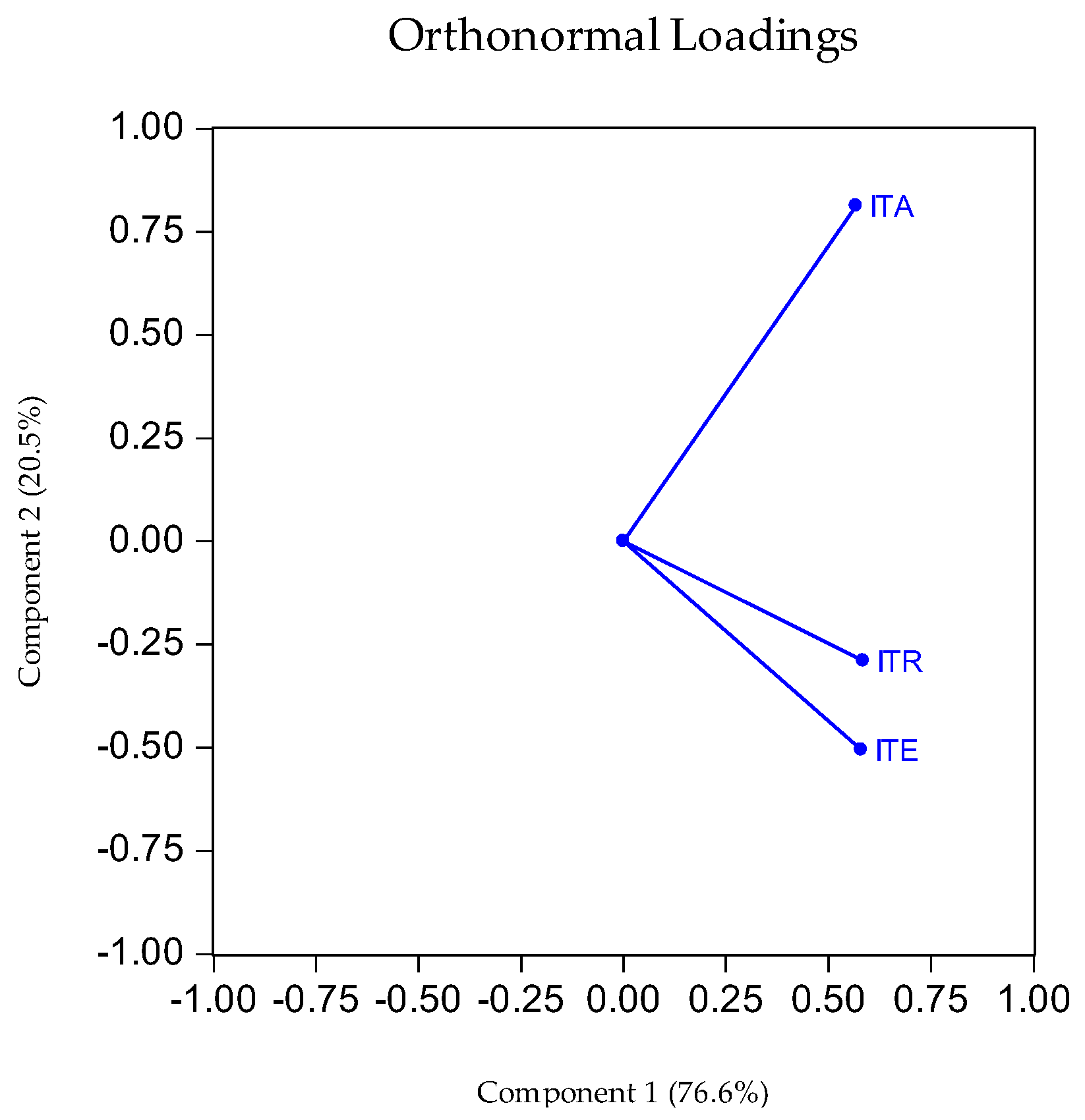
Eigenvectors (loadings)			PC 1	PC 2	PC 3
International tourism number of arrivals (ITA)			0.485280	0.862677	0.142450
International tourism expenditures (ITE)			0.603986	−0.448543	0.658795
International tourism receipts (ITR)			0.632222	−0.233662	−0.738713
Ordinary correlations:			ITA	ITE	ITR
International tourism number of arrivals (ITA)			1.000000
International tourism expenditures (ITE)			0.443870	1.000000
International tourism receipts (ITR)			0.571627	0.898522	1.000000

Source: Authors’ calculation using Eviews 10.

. Based on Kaiser’s criterion [101], we only retained the principal component with an eigenvalue greater than 1. The results show that only the first principal component should be retained, as the associated eigenvalue is λ₁ = 2.29. Opinions are divergent as regards the threshold for the cumulative proportion of variance. For social sciences, the literature suggests that the explained variance should represent at least 60% of the total one [106]. As seen in Table 3, the share of the first principal component’s variance in the total one is 76.57%, the second has a share of 20.47% and the third—2.95%.

As can be seen on the cumulative proportion column, the first principal component preserves 76.57% of the information of the original variables. Thus, by reducing the dimensionality of our original variables from 3 to 1, we manage to retain at the same time almost 80% of the original information, without losing much information.

To identify the variables with the greatest influence on each component, a loading plot was used, as seen in Figure 1. Loadings range from −1 to 1, with values close to −1 or 1 indicates a strong influence on the component, and values close to 0 indicate a weak influence. The plot shows the strongly correlated variables within the two components’ coordinate system, allowing for the determination of the nature of each principal component. Component 1 is highly correlated with all three variables, with loadings closer to 1.

Table 3’s second part displays the eigenvectors associated with each principal eigenvalue and the share of the eigenvector length associated with each variable. These values are used to estimate the principal component scores and consist of coefficients corresponding to each variable. A variable’s importance in a principal component is proportional to the absolute value of the associated coefficient. The relative importance of a variable is evaluated by the share of the length of its eigenvector. Only PC1 has positive coefficients, whereas PC2 and PC3 have negative coefficients with low influence. As a consequence, the composite index will be constructed using only the first principal component.

Table 3’s last section shows the ordinary correlation between the three variables that were used in the estimation.

The results suggest that international tourism arrivals have a medium and positive impact both on the international tourism expenditures (0.44) as well as on the international tourism receipts (0.57), while international tourism expenditures and international tourism receipts exhibit a strong and positive correlation (0.89) for EU countries.

4.3. ARDL Model

The first step in the ARDL procedure is the investigation of the stationarity of each variable. We have used the ARDL/Bounds Testing methodology proposed by Pesaran and Shin [108] and Pesaran et al. [109]. All the variables should be either stationary or present a single unit root—I(1). Some studies [120] also recommend that the dependent variable is I(1); this is not a condition widely accepted in the literature, but in our case, it is observed.

We analyzed the pattern of the variables and tested the significance of the trend and constant coefficients in the unit root regressions. Dickey Fuller [110], Phillips, and Perron [111] unit root tests confirmed that the series are either stationary or integrated of first degree. Levin, Lin, and Choo [112] unit root test was used to investigate wether a common unit root process is present in the data.

Table 4. Panel data unit root tests.

	Tourism Index Trend, Constant		CO2 Emissions Trend, Constant		Energy Intensity Constant		Trade Openness Trend, Constant		Gdp Per Capita Trend, Constant
	I(0)	I(1)	I(0)	I(1)	I(0)	I(1)	I(0)	I(1)	I(0)	I(1)
LLC	−0.65	−8.90 *	−2.48	−15.5 *	−3.32 *	-	−3.11 *	-	−3.85 *	-
ADF	53.38	117.33 *	70.14	317.3 *	86.75 *	-	92.86 *	-	70.07 *	-
PP	49.88	299.78 *	65.8	708.25 *	86.23 *	-	72.43 *	-	33.56	159.56 *

The null hypothesis states that the unit root exists. The asterisks * indicate the rejection of the null hypothesis at the 0.01 level. I(0) indicates at the level and I(1) at first diference. Source: Authors’ calculation using Eviews 10.

presents the results of these tests as well as the models employed for the investigation of the stationarity of each variable—for example, panel data unit root test for tourism index was run under the assumption of the presence of an intercept and deterministic trend. The results confirm that we may apply the bound test for cointegration.

Multicoliniarity between the independent variables might affect the results of our empirical analysis. Variance inflation factor (VIF) is a measure of the amount of multicoliniarity that is often employed in the literature. The higher the VIF value, the stronger the correlation of the variable with the others is. The optimum value for VIF is below 10, but some researchers state that if the value is above 5, the regression is highly correlated.

The coefficients in

Table 5. Variance inflation factor values.

Variable	Coeficient Variance	Uncentered VIF	Centered VIF
TO	0.010690	212.0992	2.232115
GDP	0.000661	69.94630	1.140769
EI	0.001285	14.23313	2.291688
CO2	0.008263	30.85850	1.267843
C	0.246351	228.7455	NA

Source: Authors’ calculation using Eviews 10.

indicate that there is no multicolliniarity between the independent variables considered for our model—GDP growth rate, CO₂ emissions, trade openness as well as the energy efficiency. All the centered VIF values are below 2.5, which is a threshold accepted for the absence of multicoliniarity. Spearman’s rho rank order correlation coefficients were computed and as seen in

Table 6. Spearman’s rho rank order correlation.

Correlation (Probability)	Tourism Index	Trade Openness	GDP Per Capita	Energy Intensity	CO2 Emissions
Tourism index	1.000000 (-----)
Trade openness	−0.303361 (0.0000)	1.000000 (-----)
GDP per capita	0.514641 (0.0000)	0.141194 (0.0003)	1.000000 (-----)
Energy intensity	0.740634 (0.0000)	−0.583634 (0.0000)	0.280496 (0.0000)	1.000000 (-----)
CO2 emissions	0.192255 (0.0000)	0.070406 (0.0728)	0.341220 (0.0000)	0.315806 (0.0000)	1.000000 (-----)

Source: Authors’ calculation using Eviews 10.

, the results also confirmed that that there is no multicolliniarity between the selected variables.

Pesaran and Shin [109] bound test was then used in order to test the presence of a long-run relationship between the variables, which is a requirement for any model that uses non-stationary time series data. This test also has the advantage that it allows for an optimal lag order structure.

The choice of lag length can sometimes be guided by relevant economic theories or by literature. However, we decided to investigate the optimum lag length with the help of a VAR lag order selection criteria. This is an important step, because cointegration tests are sensitive to lag-length. After running an urestricted VAR model, most of the information criteria confirmed that the optimal lag length should be 1.

Pedroni Residual Cointegration test (Pedroni [113,114]) was employed to investigate the long-run relationship in our sample. We assumed that there is no deterministic trend; the outcome of the test is presented in

Table 7. Data cointegration analysis.

Alternative Hypothesis: Common AR Coefs. (within-Dimension)
	Weighted
	Statistic	Prob.	Statistic	Prob.
Panel v-Statistic	−1.265353	0.8971	−1.983460	0.9763
Panel rho-Statistic	2.107243	0.9825	3.025504	0.9988
Panel PP-Statistic	−3.894275	0.0000	−1.892562	0.0292
Panel ADF-Statistic	−2.460347	0.0069	−2.021773	0.0216
Alternative hypothesis: individual AR coefs. (between-dimension)
	Statistic	Prob.
Group rho-Statistic	4.572893	1.0000
Group PP-Statistic	−1.822481	0.0342
Group ADF-Statistic	−2.017254	0.0218

Source: Authors’ calculation using Eviews 10.

. As seen, 6 of the 11 statistics are significant at the 5% level, so the hypothesis of no cointegration is rejected. The results confirm the existence of a long-run cointegration relation between the tourism development index, CO₂ emissions, energy intensity, trade openness, and the GDP-growth rate. This means that their correlation is not short-lived, but a permanent one, and the one that can be recovered every time there is a perturbation.

Hausmann test [115] is used to differentiate between fixed effects model and random effects model, the latter being preffered due to a better efficiency. The results of the test revealed the presence of random effects, which means the PMG—Pooled Mean Group estimator is best to be used when estimating our ARDL model. The PMG estimator has the advantage that it permits the presence of heterogeneity in data in the short-run and also allows the investigation of the dynamic effects of the exogenous variables on the endogenous one at the same time.

The results presented in

Table 8. Panel ARDL model estimations.

Maximum dependent lags: 1 (Automatic selection)
Model selection method: Akaike info criterion (AIC)
Dynamic regressors (1 lag, automatic): CO2 EF GDP TO
Fixed regressors: C
Number of models evalulated: 16
Selected Model: ARDL(1, 1, 1, 1, 1)
Variable	Coefficient	Std. Error	t-Statistic	Prob.
Long Run Equation
CO2	−1.503566 ***	0.181845	−8.268393	0.0000
EF	5.062011 ***	0.517411	9.783347	0.0000
GDP	1.358501 ***	0.105167	12.91758	0.0000
TO	1.276527 ***	0.151668	8.416585	0.0000
Short Run Equation
COINTEQ01	−0.182907 ***	0.041252	−4.433850	0.0000
D(CO2)	0.140597	0.199825	0.703601	0.4820
D(EF)	−0.391181	0.282273	−1.385823	0.1664
D(GDP)	1.388396 ***	0.321982	4.312027	0.0000
D(TO)	−0.179318	0.118987	−1.507039	0.1324
C	−5.939020 ***	1.160510	−5.117594	0.0000
Mean dependent var	0.060940	S.D. dependent var	0.145331
S.E. of regression	0.107354	Akaike info criterion	−1.536175
Sum squared resid	5.647217	Schwarz criterion	−0.434151
Log likelihood	659.2570	Hannan-Quinn criter.	−1.108728

*** Coefficient is significant at the 0.01 level (2-tailed). Source: Authors’ calculation using Eviews 10.

suggest that on short-run, in all EU countries, trade openness (p = 0.1324), CO₂ emissions (p = 0.4820) and energy efficiency (p = 0.1664) do not influence the composite tourism development index, but the economic development measured by GDP (p = 0.0000) influences the index. Considering the significance of each short-run parameter, we can decide on our research hypothesis as follows: reseach hypothesis H1: For EU countries, there is a short-run relationship between the international tourism development index and GDP per capita, which is validated. Research hypothesis H2: For EU countries, there is a short-run relationship between the international tourism development index and trade openness, which is partially validated. Research hypothesis H3: For EU countries, there is a short-run relationship between international tourism development index and CO₂ emissions, which is not validated. Research hypothesis H4: For EU countries, there is a short-run relationship between international tourism development index and energy intensity, which is not validated.

As regards the long-run results, they confirm that all variables considered in our model are determinants of the composite tourism development index: CO₂ emissions have an inverse impact on the index, an improvement of the energy efficiency index, economic development, and trade openness will contribute to an increase inthe index on long-run. Research hypothesis H5: For EU countries, there is a long-run relationship between international tourism development index and GDP per capita, CO₂ emissions, energy intensity, and trade openness, which is therefore validated.

The error correction term from the long-run equation is statistically significant at the 0.01 level, and its sign is negative, which confirms the correct specification of the model.

The analysis of the cross-section results on short-run has revealed a different situation (

Table 9. Cross section short-run coefficients.

	COINTEQ01		CO2		EF		GDP		TO
Country (symbol)	Coefficient	Prob.	Coefficient	Prob.	Coefficient	Prob.	Coefficient	Prob.	Coefficient	Prob.
Austria (AUT)	−0.111535 ***	0.0000	1.453450	0.1203	−0.823635	0.5180	2.159655	0.3548	−0.808747 **	0.0363
Belgium (BEL)	−0.442010 ***	0.0000	0.448745	0.3737	−1.710581 *	0.0833	−1.621878	0.5972	−0.240584	0.2383
Bulgaria (BG)	−0.193518 ***	0.0001	1.514997	0.2160	−2.698964	0.3372	1.797699 *	0.0567	−0.667140 ***	0.0043
Cyprus (CYP)	−0.059842 ***	0.0009	−0.089950	0.9637	0.100480	0.9673	1.168575	0.1124	0.306713	0.1782
Czech Rep. (CZ)	−0.064038 ***	0.0022	−2.018545	0.1085	2.645363	0.1646	2.637793	0.1051	−0.342772 **	0.0492
Germany (DE)	−0.244518 ***	0.0000	−0.196210	0.7859	−0.384496	0.6225	0.713871	0.4632	−0.003155	0.9813
Denmark (DK)	−0.391285 ***	0.0001	0.721520 *	0.0520	−1.947390	0.1381	1.980381	0.1973	−0.868476 **	0.0140
Estonia (EST)	−0.079805 ***	0.0002	0.304923 ***	0.0051	−1.588928	0.3529	1.778275	0.5651	1.071974 **	0.0262
Finland (FIN)	−0.165246 ***	0.0000	0.317788	0.4111	−0.362059	0.8428	0.114305	0.8736	0.407848 *	0.0788
France (FR)	−0.224635 ***	0.0006	−1.648408	0.1055	1.472268	0.2819	6.954619	0.1432	−1.630731 ***	0.0079
Greece (GRe)	−0.064548 ***	0.0006	−0.983155	0.5818	−0.074232	0.9793	1.323175	0.1567	0.989505 ***	0.0031
Croatia (HR)	−0.271757 ***	0.0003	0.506202	0.2829	−1.211727	0.2947	1.472090	0.2427	−0.054047	0.6813
Hungary (HU)	−0.095681 ***	0.0001	−0.102844	0.9251	0.516979	0.7851	0.642600	0.3947	−0.033438	0.6632
Ireland (IRL)	−0.019872 ***	0.0003	−1.220823	0.1229	1.838948 *	0.0626	0.186116	0.2365	−1.096964 ***	0.0008
Italy (IT)	−0.070857 ***	0.0001	−0.116307	0.7186	−0.131739	0.7766	1.440686	0.4652	−0.173779	0.1743
Latvia (LTV)	−1.034161 ***	0.0000	−0.606340	0.1239	−1.404111	0.1421	−1.136716 ***	0.0027	0.026138	0.7478
Luxemburg (LUX)	−0.037176 ***	0.0001	−0.560233	0.7281	1.720675	0.6034	1.317853	0.1938	−0.786167 **	0.0299
Lithuania (LIT)	−0.191021 ***	0.0000	−0.459581	0.3568	0.202021	0.5492	1.231903	0.3209	0.058787	0.7864
Malta (MT)	−1.065451 ***	0.0000	0.508904	0.3231	−3.580252 *	0.0501	−1.597735 ***	0.0034	−0.040867	0.7429
Holland (NLD)	−0.028852 ***	0.0000	0.098864 **	0.0149	−0.057914	0.1241	−0.278674 **	0.0480	0.150437 **	0.0140
Poland (PL)	−0.147930 ***	0.0010	−0.516685	0.6467	0.269253	0.8243	0.625520	0.7473	−0.418472	0.1771
Portugal (PRT)	−0.09594 ***	0.0000	2.738404	0.5905	−1.575288	0.7670	3.617243	0.2034	0.006463	0.9807
Romania (RO)	−0.092524 ***	0.0001	0.682499	0.1659	−1.798529	0.4387	2.069539	0.2854	0.473470 *	0.0614
Slovakia (SK)	−0.002114	0.6459	1.350931	0.3358	−0.139917	0.9489	2.149113 *	0.0851	0.284015	0.2353
Slovenia (SLV)	−0.227743 ***	0.0000	0.841964	0.1487	−1.463140	0.1532	2.007209 **	0.0344	−0.351199 **	0.0332
Sweden (SWE)	−0.198152 ***	0.0000	−0.017377	0.9368	0.374430	0.4957	0.234686	0.5916	−0.254177 *	0.0555
Spain (ESP)	−0.169529 ***	0.0002	0.096443	0.2307	0.237670	0.4016	1.973688 *	0.0771	−0.640754 **	0.0280

*** Coefficient is significant at the 0.01 level (2-tailed). ** Coefficient is significant at the 0.05 level (2-tailed). * Coefficient is significant at the 0.1 level (2-tailed). Source: Authors’ calculation using Eviews 10.

). CO₂ emissions have an insignificant influence on the composite tourism development index in the majority of countries (except for Denmark, Estonia and Holland). Trade openness has a significant short-run influence on the index in most cases. In Austria, Bulgaria, Czech Republic, Denmark, France, Ireland, Luxembourg, Slovenia, Sweden, and Spain, openness negatively influences the composite tourism development index, while the impact of trade openness in Estonia, Greece, Holland, and Romania is direct. Energy efficiency influences the composite tourism development index on short-run only in several countries. In Belgium and Malta, the energy efficiency has a positive impact on the short-run; while in Ireland, the energy efficiency has a negative impact on the composite tourism development index.

As regards the influence of GDP on the composite tourism index in each of the EU27 countries, the results reveal that only in Bulgaria, Malta, Holland, Slovenia, Slovakia, and Spain, the correlation is statistically significant. The scatterplots and regression lines for each EU country that reveal the correlation between the two variables can be found in Appendix A.

We also performed diagnostics tests in order to ensure the validity of the model. Even though the normality hypothesis was rejected, the results are not biased (Thadewald and Bunning, [121]).

As regards the causality analysis performed on our data, we have started with the investigation of the cross-sectional dependence in the panel data. In addition to the heterogeneity among cross-sections, cross-sectional dependence is also present.

In case that the null hypothesis cannot be rejected, it means there is no Granger causality among some of the individuals (not all) in the panel, so Dumitrescu-Hurlin [40] causality test allows for differences among them. However, the rejection of the null hypothesis reflects the fact that there is Granger causality for all individuals in the panel, which means Granger causality results are homogenous across the panel. These new hypotheses have been formulated under certain assumptions (e.g., in case of a causal relationship between a given number of individuals, a set of parameters should be identical); to solve the problems issued by these, Dumitrescu and Hurlin compute the average Wald value, which is the mean of the Wald statistics computed after determining the Granger regressions for each individual. They demonstrated that the standardized statistics associated with the average Wald value, ($\overline{\mathrm{Z}}$), are normally distributed N(0,1). The decision of the test is based on the comparison of $\overline{\mathrm{Z}}$ with the standard critical values, in case the number of individuals and periods of time are large enough. In cases the number of periods is relatively small, the use of the estimated standardized statistic $\tilde{\mathrm{Z}}$ is recommended, which is also normally distributed.

As seen in

Table 10. Dumitrescu-Hurlin Panel Causality Test.

Null Hypothesis:	W-Stat.	Zbar-Stat.	Prob.
TO does not homogeneously cause TI	3.29149	2.08155 **	0.0374
TI does not homogeneously cause TO	3.13075	1.76030 *	0.0784
EF does not homogeneously cause TI	2.92630	1.35167	0.1765
TI does not homogeneously cause EF	3.84341	3.18463 ***	0.0014
CO2 does not homogeneously cause TI	3.06471	1.62831 *	0.1035
TI does not homogeneously cause CO2	5.52232	6.54015 ***	6 × 10−11
GDP does not homogeneously cause TI	7.43691	10.3667 ***	0.0000
TI does not homogeneously cause GDP	3.15634	1.81143 *	0.0701

*** Coefficient is significant at the 0.01 level (2-tailed). ** Coefficient is significant at the 0.05 level (2-tailed). * Coefficient is significant at the 0.1 level. Source: Authors’ calculation using Eviews 10.

, Z bar values are in almost all cases greater in absolute value than the critical values for the 1%, 5% or 10% level of significance. For example, the null hypothesis “TO does not homogeneously cause TI” is rejected for a 5% level of significance, since the p value is 0.0374 < 0.05., The null hypothesis “TI does not homogeneously cause TO” is rejected for a 10% level of significance, since the p value is 0.0784 < 0.1. This means there is a homogenous bidirectional causality between trade openness and tourism development index.

To summarize, Dumitrescu-Hurlin causality test confirm feedback homogenous bidirectional causality between tourism development index and trade openness, between tourism development index and CO₂ emissions, and between tourism development index and GDP and unilateral homogenous causality running from tourism development index to energy efficiency. In addition, since the null hypothesis cannot be rejected for the unilateral causality from energy efficiency towards the international tourism development index, heterogenous causality exists among the countries in our sample.

This is why we conclude that research hypothesis H6: For EU countries, there is feedback causality between tourism and GDP per capita, CO₂ emissions, energy intensity, and trade openness, which is partially validated.

5. Discussion, Policy Implications and Limitations

5.1. Tourism and Economic Growth

Tourism has long been recognized as a powerful driver of economic growth and development, especially in countries where it represents a significant share of the economy. The correlation between tourism and economic growth is complex, and it involves several factors. Thus, tourism has become an increasingly important component of national economic development strategies as policy makers seek to harness the industry’s potential to create jobs, stimulate growth, and promote sustainable development. However, the correlation between tourism and economic growth is not always straightforward and can be influenced by several factors such as government policies, environmental considerations, and global economic conditions. Understanding the nature of this relationship is therefore crucial for policy makers who wish to maximize the economic benefits of tourism while mitigating its potential negative impacts.

International tourism can contribute to economic growth by generating foreign exchange incomes, creating employment opportunities, and stimulating investment in infrastructure and related industries such as hospitality, transport, and entertainment. This can be particularly important for developing countries, where international tourism can be a major source of income and a driver of economic development. In the present study, we were able to ascertain the fact that in the case of the EU27 panel, economic growth influences international tourism both in the shortrun and in the longrun. Regarding the cross-section analysis, it was found that the economic growth measured with the help of the GDP influences international tourism both in the shortrun and in the longrun, only in Malta, the Netherlands, Slovenia, and Spain, while in the other countries, economic growth influences tourism only in the longrun, with the exception of Slovenia, where a short-run relationship between the two indicators was identified. Therefore, the hypothesis of tourism-led growth is supported in the case of EU countries and verifies many empirical studies that have found a positive relationship between tourism and economic growth, although the strength of this relationship may vary depending on factors such as the level of economic development, size and the nature of tourism, the industry, and the quality of tourism infrastructure. The results of the study also showed a two-dimensional relationship between tourism and economic growth, this result being in accordance with a series of articles identified in the specialized literature [19,38,39]. Therefore, we can state that economic growth can lead to an increase in tourism activity because of increased incomes, higher levels of consumer spending and higher disposable incomes. This, in turn, can generate additional economic growth by creating employment opportunities, promoting investment in tourism-related infrastructure, and contributing to tax revenues. On the other hand, tourism can also contribute to economic growth by providing a source of foreign exchange earnings, creating jobs and incomes, and generating multiplier effects in other sectors of the economy. However, it is important to note that economic growth alone may not be sufficient to guarantee the sustainable development of tourism. Other factors such as environmental protection, natural and cultural resources, and the quality of the tourist product, also play a significant role in attracting and retaining tourists in EU countries. Therefore, it is essential to balance economic growth and sustainable tourism development to ensure the long-run viability of the tourism industry in these countries.

The relationship between tourism, economic growth, environment, and trade openness has a high degree of complexity. The impact of economic growth on tourism can have several policy implications. Greater focus by policymakers on promoting economic growth to boost tourism could encourage entrepreneurship, innovation, and investment in tourism-related infrastructure such as hotels, airports, and transport systems. In addition, in order to mitigate the negative effects of tourism on the environment, while promoting economic growth in the sector, a series of policy implications could be mentioned such as the adoption of sustainable practices that reduce the negative impacts of tourism on the environment by promoting ecotourism, reducing waste and pollution and encouraging the use of renewable energy sources; investing in green infrastructure such as public transport, cycling and walking routes and charging stations for electric vehicles; public education campaigns, ecological tourism certifications and the promotion of sustainable tourism alternatives in order to increase public awareness of the impact of tourism on the environment.

5.2. Tourism and Environment

The issue of energy consumption and tourism deals with energy consumption contributing significantly to greenhouse gas emissions and pollution. The availability and affordability of energy are crucial to support tourism activities and infrastructure development. The results of the ARDL model showed that long-run energy intensity had a favorable influence on the tourism development index in EU27 countries, while the CO₂ emission had a negative influence on the tourism development index. Policies for energy consumption in the tourism sector should take into account both its positive and negative impacts [67,71]. Governments and tourism operators should prioritize investments in renewable energy sources and energy-efficient technologies in order to reduce the environmental footprint of tourism activities. In addition, promoting sustainable tourism practices such as low-carbon transport, eco-friendly accommodation, and responsible tourist behavior can help reduce energy consumption and greenhouse gas emissions. Policy makers should explore ways to stimulate the adoption of sustainable practices and technologies by offering tax credits or other forms of financial support.

5.3. Tourism and Trade Openness

Trade openness can have a positive impact on tourism by promoting the flow of tourists and increasing the competitiveness of the tourism industry in a country. The results of the study showed that at the level of panel data, trade openness influences tourism in a positive sense, and this influence is statistically significant only in the longrun [74,75]. Regarding the causal relationship, our research is in accordance with that of Hussain [68], between trade openness and tourism development index, there is a statistically significant bidirectional relationship. The relationship between trade openness and tourism is mutually beneficial, as tourism can also stimulate trade and economic growth. Greater opening of markets to foreign goods and services can lead to an increase in the availability of tourism-related products and services, such as accommodation, restaurants, and attractions, which would stimulate the economy by creating jobs and increasing income from tourism and tourism-related activities. Furthermore, trade openness can also help attract foreign investment in the tourism sector. The policy implications of this relationship include the need for countries to pursue policies that promote trade openness while supporting the development of their tourism industry.

5.4. Limitations

One significant limitation of our study is the relatively short period of the available time series data, which is a common issue in similar analyses. Tourism indicators in UE countries have data starting from 1995, and for energy intensity index, the most recent data available are from 2019. The presence of missing data is a challenge faced by many databases, and it requires either the removal of incomplete observations or the use of imputation techniques to estimate missing values based on available information. Both methods can potentially impact the conclusions drawn from the database analysis. Additionally, our study is limited by the absence of data for indicators measuring international tourism in some of the analyzed EU countries. To compensate for this limitation and have a comprehensive database, we calculated missing values for some EU countries.

6. Conclusions

In our study, we investigated the relationship between the tourism development index and GDP per capita, CO₂ emissions, energy intensity index, and trade openness in a panel of 26 European Union countries. To assess tourism development, we constructed a weighted index using principal component analysis to combine information from three indicators into a single factor. We then analyzed the short- and long-run relationships between this index and GDP per capita, CO₂ emissions, energy intensity index, and trade openness using an ARDL model for panel data. The following conclusions can be drawn from our empirical analysis:

• In the shortrun, at the panel level, only GDP per capita has a statistically significant impact on the tourism index.
• CO₂ emissions, energy intensity index, and trade openness do not influence the tourism index in the shortrun.
• In the longrun, all indicators have a statistically significant impact on the tourism index. Specifically, CO₂ emissions have a negative effect, while GDP per capita, energy consumption, and trade openness have a positive effect.
• As regards the causal relationships between these indicators, we applied the Dumitrescu- Hurlin test. At the panel level, the results indicate a bidirectional homogenous causality between the tourism index and GDP per capita, between tourism index and trade openness, and between tourism index and CO₂ emissions. As regards the energy intensity—international tourism development index causality, Dumitrescu-Hurlin test confirms unilateral homogenous causality running from tourism development index to energy efficiency. In addition, since the null hypothesis cannot be rejected for the unilateral causality from energy efficiency towards the international tourism development index, there is heterogenous Granger causality among some, but not in all countries in our sample.

Our study partially confirms previous research in this field, motivating us to further investigate the topic. In our future research, we aim to consider additional key determinants such as exchange rates, destination prices, transport infrastructure, population, and more. Furthermore, we intend to extend the analysis to cover longer time periods if possible.

References

- European Travel Commission. Available online: https://etc-corporate.org/ (accessed on 4 March 2023).
- Dogru, T.; Sirakaya-Turk, E. Engines of Tourism’s Growth: An Examination of Efficacy of Shift-Share Regression Analysis in South Carolina. Tour. Manag. 2017, 58, 205–214. [Google Scholar] [CrossRef]
- Liu, Y.; Sadiq, F.; Ali, W.; Kumail, T. Does Tourism Development, Energy Consumption, Trade Openness and Economic Growth Matters for Ecological Footprint: Testing the Environmental Kuznets Curve and Pollution Haven Hypothesis for Pakistan. Energy 2022, 245, 123208. [Google Scholar] [CrossRef]
- Nguyen, Q.H. Impact of Investment in Tourism Infrastructure Development on Attracting International Visitors: A Nonlinear Panel ARDL Approach Using Vietnam’s Data. Economies 2021, 9, 131. [Google Scholar] [CrossRef]
- Lahura, E.; Sabrera, R. The Effect of Infrastructure Investment on Tourism Demand: A Synthetic Control Approach for the Case of Kuelap, Peru. Empir. Econ. 2022, 1–36. [Google Scholar] [CrossRef] [PubMed]
- Scott, D.; Gössling, S.; Hall, C.M. International Tourism and Climate Change. WIREs Clim. Change 2012, 3, 213–232. [Google Scholar] [CrossRef]
- Sæþórsdóttir, A.D.; Hall, C.M. Visitor Satisfaction in Wilderness in Times of Overtourism: A Longitudinal Study. J. Sustain. Tour. 2021, 29, 123–141. [Google Scholar] [CrossRef]
- Leal Filho, W.; Ng, A.W.; Sharifi, A.; Janová, J.; Özuyar, P.G.; Hemani, C.; Heyes, G.; Njau, D.; Rampasso, I. Global Tourism, Climate Change and Energy Sustainability: Assessing Carbon Reduction Mitigating Measures from the Aviation Industry. Sustain. Sci. 2023, 18, 983–996. [Google Scholar] [CrossRef]
- Le, T.-H.; Chang, Y.; Park, D. Trade Openness and Environmental Quality: International Evidence. Energy Policy 2016, 92, 45–55. [Google Scholar] [CrossRef]
- Lanza, A.; Pigliaru, F. Tourism and Economic Growth: Does Country’s Size Matter? Riv. Int. Sci. Econ. E Commer. 2000, 47, 77–85. [Google Scholar]
- Lanza, A.; Pigliaru, F. Why Are Tourism Countries Small and Fast-Growing? In Tourism and Sustainable Economic Development; Kluwer Academic Publishers: New York, NY, USA, 2000; pp. 57–69. [Google Scholar]
- Balaguer, J.; Cantavella-Jordá, M. Tourism as a Long-Run Economic Growth Factor: The Spanish Case. Appl. Econ. 2002, 34, 877–884. [Google Scholar] [CrossRef]
- Antonakakis, N.; Dragouni, M.; Filis, G. How Strong Is the Linkage between Tourism and Economic Growth in Europe? Econ. Model. 2015, 44, 142–155. [Google Scholar] [CrossRef]
- Cárdenas-García, P.J.; Sánchez-Rivero, M.; Pulido-Fernández, J.I. Does Tourism Growth Influence Economic Development? J. Travel Res. 2015, 54, 206–221. [Google Scholar] [CrossRef]
- Nowak, J.-J.; Sahli, M.; Cortés-Jiménez, I. Tourism, Capital Good Imports and Economic Growth: Theory and Evidence for Spain. Tour. Econ. 2007, 13, 515–536. [Google Scholar] [CrossRef]
- Eeckels, B.; Filis, G.; Leon, C. Tourism Income and Economic Growth in Greece: Empirical Evidence from Their Cyclical Components. Tour. Econ. 2012, 18, 817–834. [Google Scholar] [CrossRef]
- Bayramoğlu, T.; Arı, Y.O. The Relationship between Tourism and Economic Growth in Greece Economy: A Time Series Analysis. Comput. Methods Soc. Sci. 2015, 3, 89–93. [Google Scholar]
- Proença, S.; Soukiazis, E. Tourism as an Economic Growth Factor: A Case Study for Southern European Countries. Tour. Econ. 2008, 14, 791–806. [Google Scholar] [CrossRef]
- Cortes-Jimenez, I.; Pulina, M. Inbound Tourism and Long-Run Economic Growth. Curr. Issues Tour. 2010, 13, 61–74. [Google Scholar] [CrossRef]
- Aslan, A. Tourism Development and Economic Growth in the Mediterranean Countries: Evidence from Panel Granger Causality Tests. Curr. Issues Tour. 2014, 17, 363–372. [Google Scholar] [CrossRef]
- Chou, M.C. Does Tourism Development Promote Economic Growth in Transition Countries? A Panel Data Analysis. Econ. Model. 2013, 33, 226–232. [Google Scholar] [CrossRef]
- Surugiu, C.; Surugiu, M.R. Is the Tourism Sector Supportive of Economic Growth? Empirical Evidence on Romanian Tourism. Tour. Econ. 2013, 19, 115–132. [Google Scholar] [CrossRef]
- Bento, J.P.C. Tourism and Economic Growth in Portugal: An Empirical Investigation of Causal Links. Tour. Manag. Stud. 2016, 12, 164–171. [Google Scholar] [CrossRef]
- Demirhan, B. Tourism-Led Growth Hypothesis in Mediterranean Countries: Evidence from a Panel Cointegration and Error Correction Model. Appl. Econ. Financ. 2015, 3, 38–53. [Google Scholar] [CrossRef]
- Šimundić, B.; Kuliš, Z. Tourism and Economic Growth in Mediterranean Region: Dynamic Panel Data Approach. Acta Econ. Tur. 2016, 2, 65–84. [Google Scholar] [CrossRef]
- Selimi, N.; Sadiku, S.L.; Sadiku, M. The Impact of Tourism on Economic Growth in the Western Balkan Countries: An Empirical Analysis. Int. J. Bus. Econ. Sci. Appl. Res. 2017, 10, 19–25. [Google Scholar] [CrossRef]
- Kuliš, Z.; Šimundić, B.; Pivčević, S. The Analysis of Tourism and Economic Growth Relationship in Central and Eastern European Countries. In Economy, Finance and Business in Southeastern and Central Europe; Karasavvoglou, A., Goić, S., Polychronidou, P., Delias, P., Eds.; Springer Proceedings in Business and Economics; Springer International Publishing: Cham, Switzerland, 2018; pp. 537–551. [Google Scholar] [CrossRef]
- Tang, C.F.; Tan, E.C. Tourism-Led Growth Hypothesis: A New Global Evidence. Cornell Hosp. Q. 2018, 59, 304–311. [Google Scholar] [CrossRef]
- Fonseca, N.; Sánchez Rivero, M. Granger Causality between Tourism and Income: A Meta-Regression Analysis. J. Travel Res. 2020, 59, 642–660. [Google Scholar] [CrossRef]
- Škrinjarić, T. Stock Market Reactions to Brexit: Case of Selected CEE and SEE Stock Markets. Int. J. Financ. Stud. 2019, 7, 7. [Google Scholar] [CrossRef]
- Tung, L.T. The Tourism-Led Growth Hypothesis in Transition Economies? Empirical Evidence from a Panel Data Analysis. Geoj. Tour. Geosites 2021, 38, 1076–1082. [Google Scholar] [CrossRef]
- Lee, C.-C.; Chang, C.-P. Tourism Development and Economic Growth: A Closer Look at Panels. Tour. Manag. 2008, 29, 180–192. [Google Scholar] [CrossRef]
- Oh, C.-O. The Contribution of Tourism Development to Economic Growth in the Korean Economy. Tour. Manag. 2005, 26, 39–44. [Google Scholar] [CrossRef]
- Katircioglu, S.T. Revisiting the Tourism-Led-Growth Hypothesis for Turkey Using the Bounds Test and Johansen Approach for Cointegration. Tour. Manag. 2009, 30, 17–20. [Google Scholar] [CrossRef]
- Payne, J.E.; Mervar, A. The Tourism–Growth Nexus in Croatia. Tour. Econ. 2010, 16, 1089–1094. [Google Scholar] [CrossRef]
- Dritsakis, N. Tourism as a Long-Run Economic Growth Factor: An Empirical Investigation for Greece Using Causality Analysis. Tour. Econ. 2004, 10, 305–316. [Google Scholar] [CrossRef]
- Apergis, N.; Payne, J.E. Tourism and Growth in the Caribbean–Evidence from a Panel Error Correction Model. Tour. Econ. 2012, 18, 449–456. [Google Scholar] [CrossRef]
- Tugcu, C.T. Tourism and Economic Growth Nexus Revisited: A Panel Causality Analysis for the Case of the Mediterranean Region. Tour. Manag. 2014, 42, 207–212. [Google Scholar] [CrossRef]
- Dogru, T.; Bulut, U. Is Tourism an Engine for Economic Recovery? Theory and Empirical Evidence. Tour. Manag. 2018, 67, 425–434. [Google Scholar] [CrossRef]
- Dumitrescu, E.-I.; Hurlin, C. Testing for Granger Non-Causality in Heterogeneous Panels. Econ. Model. 2012, 29, 1450–1460. [Google Scholar] [CrossRef]
- Kim, H.J.; Chen, M.-H.; Jang, S.S. Tourism Expansion and Economic Development: The Case of Taiwan. Tour. Manag. 2006, 27, 925–933. [Google Scholar] [CrossRef]
- Ozturk, I.; Acaravci, A. On the Causality between Tourism Growth and Economic Growth: Empirical Evidence from Turkey. Transylv. Rev. Adm. Sci. 2009, 25E, 73–81. [Google Scholar]
- Kasimati, E. Economic Impact of Tourism on Greece’s Economy: Cointegration and Causality Analysis. Int. Res. J. Financ. Econ. 2011, 79, 79–85. [Google Scholar]
- Tang, C.-H.; Jang, S. The Tourism–Economy Causality in the United States: A Sub-Industry Level Examination. Tour. Manag. 2009, 30, 553–558. [Google Scholar] [CrossRef]
- Brida, J.G.; Monterubbianesi, P.D.; Aguirre, S.Z. The Impacts of Tourism on Economic Growth and Development: The Case of the Main Colombian Destinations. PASOS Rev. Tur. Patrim. Cult. 2011, 9, 291–303. [Google Scholar]
- Jacobson, S.K.; Robles, R. Ecotourism, Sustainable Development, and Conservation Education: Development of a Tour Guide Training Program in Tortuguero, Costa Rica. Environ. Manag. 1992, 16, 701–713. [Google Scholar] [CrossRef]
- Milne, S. Tourism and Development in South Pacific Microstates. Ann. Tour. Res. 1992, 19, 191–212. [Google Scholar] [CrossRef]
- Meyer, E. Beeinflussung Der Fauna Alpiner Böden Durch Sommer- Und Wintertourismus in West-Österreich (Ötztaler Alpen, Rätikon). Rev. Suisse Zool. 1993, 100, 519–527. [Google Scholar] [CrossRef]
- Havlikova, M.; Sobotkova, A. Impacts of Tourism on Natural Environment-Case Study of Pla Zdarske Vrchy; Vol. Topical Issues of Tourism: Authenticity in the Context of Tourism; Vysoká škola polytechnická Jihlava: Jihlava, Czech Republic, 2018; pp. 116–124. [Google Scholar]
- Liu, L. Impacts Of Tourism Development And Tourist Activities On Environment In Scenic Ecotourism Spots. Appl. Ecol. Environ. Res. 2019, 17, 9347–9355. [Google Scholar] [CrossRef]
- Wójtowicz, B.E. Międzynarodowy Ruch Turystyczny Zagrożeniem Dla Zabytków Architektury Nabatejskiej i Społeczności Lokalnej Na Terenie Petry. Stud. Ind. Geogr. Comm. Pol. Geogr. Soc. 2018, 32, 96–107. [Google Scholar] [CrossRef]
- Yusoff, Z.B.; Zakariya, K.; Che Haron, R.; Sapian, A.R.; Asif, N.; Shakir, H.J. The Negative Impacts of Chalets Operation on the Peninsular Malaysia Marine Park Islands. Environ.-Behav. Proc. J. 2021, 6, 211–217. [Google Scholar] [CrossRef]
- Cioancă, L.-M. The Negative Impact Of Tourism In The Area Of The Bârgău Mountains Onto The Local Environment. Int. Conf. Knowl.-BASED Organ. 2015, 21, 170–178. [Google Scholar] [CrossRef]
- Weir, B. Climate Change and Tourism–Are We Forgetting Lessons from the Past? J. Hosp. Tour. Manag. 2017, 32, 108–114. [Google Scholar] [CrossRef]
- Padilla, N.A. Reflections on Global Warming and Tourism. Main Environmental Risks and Affected Tourist Regions. Entorno Geogr. 2020, 20, 1–22. [Google Scholar] [CrossRef]
- Grillakis, M.G.; Koutroulis, A.G.; Tsanis, I.K. The 2 °C Global Warming Effect on Summer European Tourism through Different Indices. Int. J. Biometeorol. 2016, 60, 1205–1215. [Google Scholar] [CrossRef] [PubMed]
- Yu, J.; Cai, W.; Zhou, M. Evaluation and Prediction Model for Ice–Snow Tourism Suitability under Climate Warming. Atmosphere 2022, 13, 1806. [Google Scholar] [CrossRef]
- Koçak, E.; Ulucak, R.; Ulucak, Z.Ş. The Impact of Tourism Developments on CO2 Emissions: An Advanced Panel Data Estimation. Tour. Manag. Perspect. 2020, 33, 100611. [Google Scholar] [CrossRef]
- Olefs, M.; Formayer, H.; Gobiet, A.; Marke, T.; Schöner, W.; Revesz, M. Past and Future Changes of the Austrian Climate–Importance for Tourism. J. Outdoor Recreat. Tour. 2021, 34, 100395. [Google Scholar] [CrossRef]
- Shani, A.; Arad, B. Climate Change and Tourism: Time for Environmental Skepticism. Tour. Manag. 2014, 44, 82–85. [Google Scholar] [CrossRef]
- Hall, C.M.; Amelung, B.; Cohen, S.; Eijgelaar, E.; Gössling, S.; Higham, J.; Leemans, R.; Peeters, P.; Ram, Y.; Scott, D.; et al. No Time for Smokescreen Skepticism: A Rejoinder to Shani and Arad. Tour. Manag. 2015, 47, 341–347. [Google Scholar] [CrossRef]
- Schweinsberg, S.; Darcy, S. Climate Change, Time and Tourism Knowledge: The Relativity of Simultaneity. Sustainability 2022, 14, 16220. [Google Scholar] [CrossRef]
- Hanna, P.; Scarles, C.; Cohen, S.; Adams, M. Everyday Climate Discourses and Sustainable Tourism. J. Sustain. Tour. 2016, 24, 1624–1640. [Google Scholar] [CrossRef]
- Qiao, G.; Gao, J. Chinese Tourists’ Perceptions of Climate Change and Mitigation Behavior: An Application of Norm Activation Theory. Sustainability 2017, 9, 1322. [Google Scholar] [CrossRef]
- Gössling, S.; Scott, D.; Hall, C.M.; Ceron, J.-P.; Dubois, G. Consumer Behaviour and Demand Response of Tourists to Climate Change. Ann. Tour. Res. 2012, 39, 36–58. [Google Scholar] [CrossRef]
- Lam-González, Y.E.; León, C.J.; De León, J. Measuring Tourist Satisfaction with Nautical Destinations: The Effects of Image, Loyalty, and Past Destination Choice. Tour. Mar. Environ. 2020, 15, 47–58. [Google Scholar] [CrossRef]
- Gössling, S.; Scott, D. The Decarbonisation Impasse: Global Tourism Leaders’ Views on Climate Change Mitigation. J. Sustain. Tour. 2018, 26, 2071–2086. [Google Scholar] [CrossRef]
- Alola, A.A.; Alola, U.V. Agricultural Land Usage and Tourism Impact on Renewable Energy Consumption among Coastline Mediterranean Countries. Energy Environ. 2018, 29, 1438–1454. [Google Scholar] [CrossRef]
- Katircioglu, S.T.; Feridun, M.; Kilinc, C. Estimating Tourism-Induced Energy Consumption and CO2 Emissions: The Case of Cyprus. Renew. Sustain. Energy Rev. 2014, 29, 634–640. [Google Scholar] [CrossRef]
- Ben Jebli, M.; Hadhri, W. The Dynamic Causal Links between CO2 Emissions from Transport, Real GDP, Energy Use and International Tourism. Int. J. Sustain. Dev. World Ecol. 2018, 25, 568–577. [Google Scholar] [CrossRef]
- Dogan, E.; Aslan, A. Exploring the Relationship among CO2 Emissions, Real GDP, Energy Consumption and Tourism in the EU and Candidate Countries: Evidence from Panel Models Robust to Heterogeneity and Cross-Sectional Dependence. Renew. Sustain. Energy Rev. 2017, 77, 239–245. [Google Scholar] [CrossRef]
- Isik, C.; Dogru, T.; Turk, E.S. A Nexus of Linear and Non-Linear Relationships between Tourism Demand, Renewable Energy Consumption, and Economic Growth: Theory and Evidence. Int. J. Tour. Res. 2018, 20, 38–49. [Google Scholar] [CrossRef]
- Demir, E.; Gozgor, G.; Paramati, S.R. To What Extend Economic Uncertainty Effects Tourism Investments? Evidence from OECD and Non-OECD Economies. Tour. Manag. Perspect. 2020, 36, 100758. [Google Scholar] [CrossRef]
- Katircioglu, S. Tourism, Trade and Growth: The Case of Cyprus. Appl. Econ. 2009, 41, 2741–2750. [Google Scholar] [CrossRef]
- Lu, Z.; Gozgor, G.; Lau, C.K.M.; Paramati, S.R. The Dynamic Impacts of Renewable Energy and Tourism Investments on International Tourism: Evidence from the G20 Countries. J. Bus. Econ. Manag. 2019, 20, 1102–1120. [Google Scholar] [CrossRef]
- Hussain, M.N. Evaluating the Impact of Air Transportation, Railway Transportation, and Trade Openness on Inbound and Outbound Tourism in BRI Countries. J. Air Transp. Manag. 2023, 106, 102307. [Google Scholar] [CrossRef]
- Agiomirgianakis, G.M.; Sfakianakis, G. Determinants of Tourism Demand in Greece: A Panel Data Approach. Ekonometria 2014, 1, 15–26. [Google Scholar] [CrossRef]
- Surugiu, C.; Leitão, N.C.; Surugiu, M.R. A Panel Data Modelling of International Tourism Demand: Evidences for Romania. Econ. Res.-Ekon. Istraživanja 2011, 24, 134–145. [Google Scholar] [CrossRef]
- Ibrahim, M.A.M.A. The Determinants of International Tourism Demand for Egypt: Panel Data Evidence. Eur. J. Econ. Financ. Adm. Sci. 2011, 30, 51–58. [Google Scholar] [CrossRef]
- Turner, L.W.; Witt, S.F. Factors Influencing Demand for International Tourism: Tourism Demand Analysis Using Structural Equation Modelling, Revisited. Tour. Econ. 2001, 7, 21–38. [Google Scholar] [CrossRef]
- Muhammad, A.; Andrews, D. Determining Tourist Arrivals in Uganda: The Impact of Distance, Trade and Origin-Specific Factors. Afr. J. Account. Econ. Financ. Bank. Res. 2008, 2, 51–62. [Google Scholar]
- Shan, J.; Wilson, K. Causality between Trade and Tourism: Empirical Evidence from China. Appl. Econ. Lett. 2001, 8, 279–283. [Google Scholar] [CrossRef]
- Roy, J. On the Environmental Consequences of Intra-Industry Trade. J. Environ. Econ. Manag. 2017, 83, 50–67. [Google Scholar] [CrossRef]
- Sinha, A.; Shahbaz, M.; Balsalobre, D. Exploring the Relationship between Energy Usage Segregation and Environmental Degradation in N-11 Countries. J. Clean. Prod. 2017, 168, 1217–1229. [Google Scholar] [CrossRef]
- Sharif Hossain, M. Panel Estimation for CO2 Emissions, Energy Consumption, Economic Growth, Trade Openness and Urbanization of Newly Industrialized Countries. Energy Policy 2011, 39, 6991–6999. [Google Scholar] [CrossRef]
- Grossman, G.; Krueger, A. Environmental Impacts of a North American Free Trade Agreement; National Bureau of Economic Research: Cambridge, MA, USA, 1991; p. w3914. [Google Scholar] [CrossRef]
- Nguyen, H.T.; Nguyen, S.V.; Dau, V.-H.; Le, A.T.H.; Nguyen, K.V.; Nguyen, D.P.; Bui, X.-T.; Bui, H.M. The Nexus between Greenhouse Gases, Economic Growth, Energy and Trade Openness in Vietnam. Environ. Technol. Innov. 2022, 28, 102912. [Google Scholar] [CrossRef]
- Sarpong, S.Y.; Bein, M.A.; Gyamfi, B.A.; Sarkodie, S.A. The Impact of Tourism Arrivals, Tourism Receipts and Renewable Energy Consumption on Quality of Life: A Panel Study of Southern African Region. Heliyon 2020, 6, e05351. [Google Scholar] [CrossRef]
- Mahrinasari, M.S.; Haseeb, M.; Ammar, J.; Meiryani, M. Does Trade Liberalization a Hazard to Sustainable Environment? Fresh Insight from ASEAN Countries. Pol. J. Manag. Stud. 2019, 19, 249–259. [Google Scholar] [CrossRef]
- Leitão, N.C.; Lorente, D.B. The Linkage between Economic Growth, Renewable Energy, Tourism, CO2 Emissions, and International Trade: The Evidence for the European Union. Energies 2020, 13, 4838. [Google Scholar] [CrossRef]
- Xue, D.; Li, X.; Ahmad, F.; Abid, N.; Mushtaq, Z. Exploring Tourism Efficiency and Its Drivers to Understand the Backwardness of the Tourism Industry in Gansu, China. Int. J. Environ. Res. Public Health 2022, 19, 11574. [Google Scholar] [CrossRef]
- Dogan, E.; Seker, F.; Bulbul, S. Investigating the Impacts of Energy Consumption, Real GDP, Tourism and Trade on CO2 Emissions by Accounting for Cross-Sectional Dependence: A Panel Study of OECD Countries. Curr. Issues Tour. 2017, 20, 1701–1719. [Google Scholar] [CrossRef]
- Ozturk, I.; Al-Mulali, U.; Saboori, B. Investigating the Environmental Kuznets Curve Hypothesis: The Role of Tourism and Ecological Footprint. Environ. Sci. Pollut. Res. 2016, 23, 1916–1928. [Google Scholar] [CrossRef]
- Badulescu, D.; Simut, R.; Mester, I.; Dzitac, S.; Sehleanu, M.; Bac, D.P.; Badulescu, A. Do Economic Growth and Environment Quality Contribute to Tourism Development in EU Countries? A Panel Data Analysis. Technol. Econ. Dev. Econ. 2021, 27, 1509–1538. [Google Scholar] [CrossRef]
- The World Bank. Available online: https://data.worldbank.org/ (accessed on 4 March 2023).
- Freudenberg, M. Composite Indicators of Country Performance: A Critical Assessment; OECD Science, Technology and Industry Working Papers 2003/16; OECD: Paris, France, 2003; Volume 2003/16. [Google Scholar] [CrossRef]
- Joint Research Centre-European Commission. Handbook on Constructing Composite Indicators: Methodology and User Guide; European Commission, Organisation for Economic Co-Operation and Development, SourceOECD (Online Service), Eds.; OECD: Paris, France, 2008.
- Pearson, K. LIII. On Lines and Planes of Closest Fit to Systems of Points in Space. Lond. Edinb. Dublin Philos. Mag. J. Sci. 1901, 2, 559–572. [Google Scholar] [CrossRef]
- Hotelling, H. Simplified Calculation of Principal Components. Psychometrika 1936, 1, 27–35. [Google Scholar] [CrossRef]
- Larose, D.T. Data Mining Methods and Models; Wiley-Interscience: Hoboken, NJ, USA, 2006. [Google Scholar]
- Kaiser, H.F. An Index of Factorial Simplicity. Psychometrika 1974, 39, 31–36. [Google Scholar] [CrossRef]
- Field, A.P. Discovering Statistics Using SPSS for Windows: Advanced Techniques for the Beginner; ISM introducing statistical methods; Sage Publications: London, UK; Thousand Oaks, CA, USA, 2000. [Google Scholar]
- Lebart, L.; Piron, M.; Morineau, A. Statistique Exploratoire Multidimensionnelle: Visualisation et Inférences en Fouille de Données, 4th ed.; Sciences SUP; Dunod: Paris, France, 2006. [Google Scholar]
- Pallant, J. SPSS Survival Manual: A Step by Step Guide to Data Analysis Using IBM SPSS, 5th ed.; McGraw Hill: Maidenhead, UK; Berkshire, UK, 2013. [Google Scholar]
- Cattell, R.B. The Scree Test For The Number Of Factors. Multivar. Behav. Res. 1966, 1, 245–276. [Google Scholar] [CrossRef]
- Nepal, R.; Indra Al Irsyad, M.; Nepal, S.K. Tourist Arrivals, Energy Consumption and Pollutant Emissions in a Developing Economy–Implications for Sustainable Tourism. Tour. Manag. 2019, 72, 145–154. [Google Scholar] [CrossRef]
- Taizeng, R.; Can, M.; Paramati, S.R.; Fang, J.; Wu, W. The Impact of Tourism Quality on Economic Development and Environment: Evidence from Mediterranean Countries. Sustainability 2019, 11, 2296. [Google Scholar] [CrossRef]
- Pesaran, M.H.; Shin, Y.; Smith, R.P. Pooled Mean Group Estimation of Dynamic Heterogeneous Panels. J. Am. Stat. Assoc. 1999, 94, 621–634. [Google Scholar] [CrossRef]
- Pesaran, M.H.; Shin, Y.; Smith, R.J. Bounds Testing Approaches to the Analysis of Level Relationships. J. Appl. Econ. 2001, 16, 289–326. [Google Scholar] [CrossRef]
- Dickey, D.A.; Fuller, W.A. Distribution of the Estimators for Autoregressive Time Series With a Unit Root. J. Am. Stat. Assoc. 1979, 74, 427. [Google Scholar] [CrossRef]
- Phillips, P.C.B.; Perron, P. Testing for a Unit Root in Time Series Regression. Biometrika 1988, 75, 335–346. [Google Scholar] [CrossRef]
- Levin, A.; Lin, C.-F.; James Chu, C.-S. Unit Root Tests in Panel Data: Asymptotic and Finite-Sample Properties. J. Econ. 2002, 108, 1–24. [Google Scholar] [CrossRef]
- Pedroni, P. Critical Values for Cointegration Tests in Heterogeneous Panels with Multiple Regressors. Oxf. Bull. Econ. Stat. 1999, 61, 653–670. [Google Scholar] [CrossRef]
- Pedroni, P. Panel Cointegration: Asymptotic and Finite Sample Properties of Pooled Time Series Tests. with an Application to the PPP Hypothesis. Econ. Theory 2004, 20, 597–625. [Google Scholar] [CrossRef]
- Hausman, J.A. Specification Tests in Econometrics. Econometrica 1978, 46, 1251. [Google Scholar] [CrossRef]
- Granger, C.W.J. Investigating Causal Relations by Econometric Models and Cross-Spectral Methods. Econometrica 1969, 37, 424. [Google Scholar] [CrossRef]
- Holtz-Eakin, D.; Newey, W.; Rosen, H.S. Estimating Vector Autoregressions with Panel Data. Econometrica 1988, 56, 1371. [Google Scholar] [CrossRef]
- Emirmahmutoglu, F.; Kose, N. Testing for Granger Causality in Heterogeneous Mixed Panels. Econ. Model. 2011, 28, 870–876. [Google Scholar] [CrossRef]
- Hair, J.F.; Anderson, R.; Tatham, R.; Black, W. Multivariate Data Analysis with Readings, 4th ed.; Prentice Hall: Englewood Cliffs, NJ, USA, 1995. [Google Scholar]
- De Vita, G.; Endresen, K.; Hunt, L.C. An Empirical Analysis of Energy Demand in Namibia. Energy Policy 2006, 34, 3447–3463. [Google Scholar] [CrossRef]
- Thadewald, T.; Büning, H. Jarque–Bera Test and Its Competitors for Testing Normality—A Power Comparison. J. Appl. Stat. 2007, 34, 87–105. [Google Scholar] [CrossRef]