Investigating the Influence of Tourism, GDP, Renewable Energy, and Electricity Consumption on Carbon Emissions in Low-Income Countries

Abstract

Due to a rapidly growing population and economy, an increase in emissions from urban growth, industrial growth, and energy use hurt the environment’s health. This research examines how tourism, population, income, renewable energy, and electricity consumption affect carbon emissions in twenty-six low-income countries. There is no cross-sectional dependence (CSD) problem, so quantile regressions (QR) and generalized method of moments (GMM) are used. Results show that the environment is obtaining benefits because of tourism. CO₂ emissions are rising because the per capita income, electricity consumption, and population are growing. CO₂ emissions can be lowered by using more renewable energy and growing the economy faster. Environmental Kuznets Curve (EKC) is also valid in low-income countries. Thus, increasing income will not be harmful to the environment. Similarly, increasing tourism, renewable energy, and rising GDP per capita benefit low-income countries. The government can focus on sustainable tourism. Policymakers may convince more people to use renewable energy resources and grow the sustainable tourism industry. This study recommends that the government reduce greenhouse gas emissions, promote tourism that is good for the environment, take initiatives to limit population growth, and use renewable energy.

1. Introduction

Tourism brings in a lot of money for countries worldwide today. It also helps the economies of the countries that send and receive tourists. Industry data show that the number of people from other countries has grown significantly over the past 30 years. Even though tourism has a significant effect on the economy, the environment is still becoming worse. In the last few decades, it has become more apparent that tourism helps the economy grow. This has made tourism more critical in both rich and developing countries. Tourism significantly affects the economies of many cities worldwide because it brings in money, taxes, jobs, and foreign currency. Brida and Pulina [1] say that tourism can make other parts of the economy more competitive through direct and indirect spillover effects. It can also create new job opportunities and help hotels save money through economies of scale. Additionally, there is proof that economies that depend too much on tourism grow slowly [2]. Tourism is essential for job creation and economic growth around the world. Before the pandemic, tourism and travel made up 10.3% of all jobs (333 million), one 1 of every 4 new jobs around the world, and 9.6% of the global (GDP) gross domestic product (containing its direct, indirect, and induced impacts). In 2019, travelers from other countries spent $1.8 trillion, 6.8% of all exports. Travel and tourism’s share of the world’s GDP dropped from 10.3% in 2019 to 5.2% in 2020 because it was harder for people to move around. The number went up from 5.9% to 6.1%. Over the next ten years, the tourism business in Sub-Saharan Africa could create almost 4 million direct jobs and 3 million indirect jobs [3,4]. During political and economic crises such as financial worries, partisan fights, and civil unrest policy uncertainty can spread to critical economic sectors such as tourism. Even though tourism is well-established in many countries with high incomes, it is only starting to reach its full potential in countries with low incomes. For example, the tourism industry in Africa is overgrowing. About 67 million people visit Africa every year. Africa is far behind other parts of the world, and only 5% of the world’s tourists went there in 2018 [5]. Given the many ways the tourist industry can help a country grow, it is essential to understand the financial, governmental, and socioeconomic factors that can help or hurt the growth of the tourism industry. Even though COVID-19 is spreading, more people visit and spend more money, showing that tourism has much room to grow. Tourism will increase in countries with low incomes. Since the 1950s, the average growth in foreign tourists yearly has been 4 to 5 percent. Even though there was a pandemic, the number of people who went to Sub-Saharan Africa rose by 8% between 2019 and 2020. The above means making it the second-fastest thriving tourist destination in the world, just after the Asia-Pacific region [6,7].

The tourist industry depends on public infrastructures such as airports, harbors, highways, railheads, and phone lines to transport people to their destinations and keep in touch with them. There are many environmental and ecological effects of building the infrastructure as well as other parts of tourist attractions such as resorts and restaurants. More and more tourists choose to travel by car. This causes severe environmental damage. Fossil fuels transport tourists to and from their destinations, in their hotels, and for other tourist-related activities. One cannot emphasize enough how vital energy is to a country’s economic growth and success. According to theoretical and real-world research, using energy helps the economy grow. This proves that using more energy can help the economy grow. However, using energy may worsen environmental damage because it increases carbon emissions. Global warming and climate change, the main topics of conversation worldwide for decades, are partly caused by carbon dioxide emissions. Climate change and global warming must stop because they harm the environment and people [8]. Several studies have been performed regarding the main things that affect carbon emissions. Even though there are different opinions, most research shows that using energy makes carbon emissions worse. On the other hand, the use of nonrenewable sources of energy seems to boost carbon dioxide emissions, while using renewable power energy seems to decrease carbon emissions [9].

Carbon emissions in developing countries must be considered more concerning and result in developing renewable energy sources. As the economy grows, people and businesses emit carbon emissions directly or indirectly. These carbon emissions are a side effect of letting out greenhouse gases. Over the years, academics and politicians have argued about how carbon emissions are related to other macroeconomic issues, how they affect the environment, and what can be executed to stop them. Real per capita income is expected to rise as the tourism industry expands and more people travel internationally. When tourists from other countries come to a country, they spend more money on goods and services, which helps other areas such as transportation and power. Thus, tourism and the economic activities that accompany it (economic expansion) have helped them grow. On the other hand, tourism has made these places more vulnerable to global warming by forcing them to use more energy and take vacations in cars powered by fossil fuels and other energy pollutants. Since the world has shrunk to the size of a village, you cannot say enough about how globalization has helped international tourism grow. Carbon emissions must be considered when determining how tourism growth affects carbon emissions. We did this investigation because of this. In addition to learning more about how tourism and emissions are related, we want to look at the causal interaction between the relevant factors. This will help us figure out if the variables we are looking at are related to each other. By figuring out the causal connection between the elements, we help the policymakers make good decisions about monetary policy that will result in long-term environmental and economic outcomes such as using renewable energy that will help current and future generations, especially in the sampled region. Using the environmental Kuznets curve (EKC), we examine whether tourism and carbon emissions are linked in Africa’s most popular tourist spots. This study looks at 26 low-income countries because there needs to be more real-world research on how tourism affects carbon emissions in low-income countries. Carbon emissions worry policymakers, researchers, and academics in the region. Since the 1970s, vast amounts of carbon dioxide have come out of these places. For example, the amount of CO₂ in the air went from 62.8% in 1980 to 65.7% in 1993 and then to 51.4% in 2014. The number of carbon emissions caused by energy and heat went from 39.8% in 1980 to 59.2% in 2001 to 54.4% in 2014 [6,7].

Our current research has three things to offer as follows: (i) This is the sole research that employs the recently developed environmental Kuznets curve (EKC) to look at the relationship between the tourism industry, wealth creation, and energy use within a multidimensional framework, especially in popular tourist spots in low-income counties. It is also one of the few papers to examine how carbon dioxide emissions affect tourism income in these countries’ most popular tourist spots, making it stand out. Lui et al. [10] said that if tourists can go to other places for the same price, they will not return to dirty and polluted areas. Because of this, carbon emissions are expected to affect the tourism industry. (ii) We add to the research by showing how the demand-flowing and supply-leading theories, which explain how tourism causes globalization and CO₂ emissions, are supported by evidence. (iii) Relying on what we found, the macroeconomic factors that cause pollution are more local, especially in the tourist areas of these countries.

This study uses the EKC hypothetic model and a modified version of Dietz and Rosa’s [11] STIRPAT model (the stochastic impacts by regression on the citizenry, affluence, and innovation) by adding income, energy, electricity production, and tourism. These are the two most important ideas in the field of environmental economics. However, when each method is looked at independently, it has significant flaws. The EKC is based on a two-variable framework with variable omission bias. As a result, empirical results are inconsistent [12]. Tourism is well fitted in the STIRPAT model [13,14]. However, the scientific community has criticized the STIRPAT model for assuming a constant link between per capita wealth and emissions (see, for instance, [15,16,17]. Thus, it is possible to combine the two theories to make a complete testing blueprint [18,19,20,21]. Per capita gross domestic product, urbanization, industrialization, and energy consumption were the controls for the baseline model.

The World Bank’s World Development Indicators (WDI) database has statistics for 26 countries for each year from 2001 to 2020, where they are available. As far as we know, ours is the first global study to examine how tourism affects the amount of carbon dioxide in the air. While previous studies have explored the impact of various factors on carbon emissions, this research explicitly targets low-income countries. By focusing on these countries, the study addresses a crucial knowledge gap. It provides tailored insights and recommendations relevant to low-income nations’ unique socioeconomic and environmental contexts. This research contributes to understanding tourism’s role in environmental sustainability. By exploring the relationship between tourism and carbon emissions in low-income countries, the study sheds light on the potential for sustainable tourism practices to minimize adverse environmental impacts and promote sustainable development. This article aims to advance knowledge by examining the effects of tourism, population, electricity consumption, and renewable energy consumption on carbon emissions in 26 low-income nations. To the best of the authors’ knowledge, this is one of the first studies to examine how tourism, population, electricity consumption, and renewable energy consumption in 26 low-income countries’ economies compare to other economic sectors regarding their added value. The research utilizes quantile regression and the generalized method of moments (GMM) as analytical methods. By employing these advanced econometric techniques, the study enhances the robustness and accuracy of the analysis, providing more nuanced insights into the relationships between the variables under investigation. However, several types of research examine the tourism- energy- income- environment literature. Only some look into how tourism affects CO₂ emissions. The research presents empirical findings and provides policy recommendations based on the study’s outcomes. By suggesting specific actions such as promoting renewable energy, implementing sustainable tourism practices, and addressing population growth and resource consumption, the research offers practical insights for policymakers and stakeholders to make informed decisions and develop adequate environmental protection and sustainable development strategies.

The subsequent sections of this research paper are organized as follows: In the next section, we will examine the existing studies conducted on the impact of tourism and various other factors on pollution. Subsequently, Section 3 explains the employed data, model, and technique. Section 4 presents the obtained results and corresponding findings. The following section, Section 5, comprehensively discusses the outcomes. Section 6 focuses on the conclusion derived from the study. The policy recommendation is expounded upon in Section 7. Finally, Section 8 delves into the study’s limitations and proposes future research directions.

2. Literature Review

Several studies have examined how tourism affects big-picture economic such as like GDP growth, urban growth, energy use, and carbon dioxide emissions [22,23,24,25,26,27]. Sherafatian–Jahromi et al. [28] used panel regression analysis and aggregated average group methods to find that CO₂ emissions in five of Southeast Asia’s most famous cities were linear or nonlinear. Rahman et al. [29] examined how tourism, fossil fuels, renewable energy, and nuclear energy use affect the environment in the most popular tourist spots worldwide. The main findings of their research showed that CSARDL accepts the EKC theory in the short and long term but does not care about it in the short and midterm. Even though the study showed that more money leads to fewer CO₂ emissions after a certain income level, the EKC happens in the CSARDL concept in the long run. Additionally, they find that using fossil fuels speeds up environmental damage and that CO₂ can be reduced by using renewable energy, nuclear energy, and more tourism. In another study, Voumik et al. [30] simulated sustainable nonrenewable and renewable energy sources for Africa’s ten most popular tourist locations using the environmental Kuznets curve (EKC) hypothesis as its foundation. The authors use panel data analysis to study the connection between CO₂ emissions, economic growth, the energy mix, and tourism. Study findings can help policymakers in Africa’s tourism sector promote sustainable energy use, reduce carbon emissions, and advance sustainable development objectives. Shakouri et al. [27] examined panel data from many Asia-Pacific countries to see how GDP growth and tourism affected CO₂ emissions. The EKC hypothesis was examined by seeing how many things fit together (GDP growth, tourism visits, fossil fuel usage, and carbon dioxide emissions). As a result, the amount of CO₂ and the number of tourists will decrease over time. Ravinthirakumaran and Ravinthirakumaran [31] examined the APEC region’s tourism industry, power use, economic growth, and carbon emissions from 1995 to 2017. To come to this conclusion, methods for computing heterogeneous panels with cross-sectional dependence were used.

When there are constant differences between the variables, they are linked across cross-sections. The variables have been related for a long time, as shown by the Westerlund multivariate cointegration test. Tourism and more energy use might lessen the effects of a growing economy, but they have almost no impact on the amount of CO₂ released into the atmosphere worldwide. The panel’s non-causality test results show that economic growth and tourism only cause CO₂ emissions in one way. The EKC hypothesis and how much it might cost to start a tourism business are controversial, but neither is an old problem. When people talk about the link between tourism and greenhouse gas emissions, this has been a big topic of conversation for a long time. Researchers have added new policy variables to the EKC framework such as electricity [32], export [33], demography [34], urban development and economic growth [9], and research and innovation [35]. As part of their research on the tourism industry using the environmental Kuznets curve (EKC) model for the United Arab Emirates (UAE) between 1984 and 2019, Majumdar and Paris [36] published an Autoregressive Distributed Lag (ARDL) model to figure out the marginal effect of tourist arrivals and underlying factors such as credit facilities to the corporate sector, urban growth, and power generation use on CO₂ emissions. Academics disagree on several things that hurt the environment. This article uses the panel cointegration method to examine how population and industrial growth affected Emissions of CO₂ in four major SAARC nations between 1980 and 2008. Researchers found that the growth of industry and population primarily caused CO₂ emissions in the selected SAARC nations. Anser et al. [37] also examined the consequences of urban development, population growth, and economic expansion in SAARC countries from 1994 to 2013. They have looked into the whole period. They used the STIRPAT model to show that CO₂ emissions are increasing in SAARC countries because their populations and GDP per person are growing. Ikram et al. [38] used several models to study the SAARC region’s CO₂ emissions, access to electricity, use of renewable energy, agricultural output, and ISO 14001 certification from 2000 to 2014. According to the report, CO₂ emissions have increased in the SAARC region because more people can access electricity. However, using renewable energy and adopting ISO 14001 can significantly cut emissions. Mehmood [39] also looked at how urbanization has affected the natural environment in SAARC countries and regions from 1996 to 2015. Using the PMG estimation method, this study found that as the SAARC region became more urban, CO₂ emissions decreased over time. From 1975 to 2018, Azam et al. [40] looked at the connections between OPEC economies’ carbon dioxide emissions, cities’ growth, and international trade. The robust least squares method and the fixed effects estimation method were used in their research. Expanding markets, using more energy, industrialization, and urbanization are all being looked into to see if they could improve the environment.

Sumaira and Siddique [41] use the common correlated effects mean group (CCEMG) and amplified average group (AAG) and estimates for the years 1984–2016 to figure out how industrialization and energy use have caused the environment in South Asian countries to become worse. The results of the analysis show that industrialization and the use of energy are two of the main reasons why the environment in South Asian countries is getting worse. Cowan et al. [42] use a panel causality test to show the link between economic development, electricity use, and CO₂ emissions in the BRICS countries between 1990 and 2010. However, when the BRICS members look at what causes what, they find different things. Awad et al. [43] looked at the link between poorness and the ecosystem again by looking at data from 91 developing countries between 1990 and 2015. Their study used the ecological footprint (EFP) instead of carbon dioxide (CO₂) emissions. For the global panel and the African region, they saw a link between poverty and the amount of damage done to the environment. Between 1995 and 2010, Gao et al. [44] looked at emission levels, energy use, economic expansion, and the growth of the tourist industry in 18 Mediterranean regions. The tourism-induced environmental Kuznets curve (EKC) was supported by cointegration analysis, which showed a long-term equilibrium link among the variables examined in the three countries. Researchers found that Northern Mediterranean countries’ GDP and economic growth were closely linked to the number of tourists who visited each year.

Kocak et al. [45] found that tourism and CO₂ emissions are related and cause each other in the top ten most visited nations. The study also found that money from tourism helped reduce CO₂. Asia, South America, and the Caribbean were all developing countries, but were not linked. Shahbaz et al. [15] use data from 1975 to 2010 to examine the associations between Bangladesh’s industrial growth, energy use, and carbon dioxide emissions. Using the ARDL bound test, the study shows that carbon intensity and industrial development have a reciprocal relationship that looks like an upside-down U. Their analysis also shows that CO₂ emissions and electricity use in Bangladesh are linked in a positive way over the long term but in a negative way over the short time. Kivyiro and Arminen [46] tried to figure out the connections between CO₂ emission levels, power generation use, cconomic growth, and foreign direct investments (FDI) in six countries in Sub-Saharan Africa. Their research in the Democratic Republic of the Congo, Kenya, and Zimbabwe showed that the environmental Kuznets curve (EKC) theory is correct. In these countries, there is a U-shaped connection between GDP per person and ecological degradation. Finally, Andjarwati et al. [47] examined how economic and energy changes affected the environment in the Association of Southeast Asian Nations (ASEAN) from 1995 to 2017.

Using an ARDL model shows that energy consumption worsens the short and long-term environment in contrast to the long-term effects of population growth, urban growth, and economic hardship. They also find that over time, urbanization makes energy use worse. Begum et al. [48] also looked at CO₂ emissions in Malaysia. They looked at 1970–1980 and how power generation use, population growth, and economic expansion changed over time. They used the ARDL bound test and concluded that Malaysia’s emissions decrease when its GDP per person increases. Ali et al. [49] used the auto-regressive distributed lag model (ARDL) bound test to examine how Nigeria’s trade openness, urbanization, energy usage, and economic expansion affected the country’s carbon emissions from 1971 to 2011. Their research showed that economic growth, energy use, and openness to trade had a more significant effect on CO₂ emissions than urban development. Additionally, Hussain et al. [50] used the fully modified ordinary least squares (FMOLS) and panel quantile regression (PQR) methods to look at how the use of nonrenewable energy and urbanization affected carbon dioxide emissions in 54 African Union countries between 1996 and 2019. If the EKC hypothesis is correct, their results will support this conclusion. Finally, the research conducted by Voumik et al. [51] investigated the effect that tourism has on the employment opportunities available to women in South America and the Caribbean. The authors use a panel data approach to examine the correlation between growth in the tourism industry and the number of women in the workforce, factoring in a wide range of economic and social conditions. This research can help guide policymakers in the region toward more equitable and sustainable tourism growth. The opposite applies to foreign direct investments (FDI), globalization, and innovation. Elfaki et al. [52] examined how industrial growth and carbon dioxide emissions changed in eight ASEAN countries between 1994 and 2018.

The literature gap for this research paper lies in the lack of comprehensive studies that specifically investigate the influence of tourism, GDP, renewable energy, and electricity consumption on pollution levels in low-income countries using advanced econometric methods such as quantile regression and generalized method of moments (GMM). While previous research has explored the relationship between these variables and pollution, few studies have focused on low-income countries specifically. The CSD test is crucial because most low-income countries are in Africa and Asia. Though low-income countries are loosely connected, the research applied the CSD test. On the other hand, most of the low-income countries are different in terms of area, economic size, energy consumption, and other factors. Thus, it is essential to check slope homogeneity. This paper applied the CSD and the SH test, the second-generation unit root and cointegration test, quantile regression, and the dynamic and system GMM. Some CSD tests show that there is no CSD problem in low-income countries. This study uses a new initiative aimed at the second generation, combining several criteria that have yet to be addressed. The authors say that, as far as they know, most of the existing research misses SH, the CSD test, and the use of typical panel estimators, all of which give incomplete results. Furthermore, the application of quantile regression and GMM methods offers a robust and nuanced analysis by considering different quantiles of pollution levels and accounting for potential endogeneity issues, respectively. Therefore, this research aims to fill this gap by thoroughly examining the abovementioned variables’ impact on pollution in low-income countries using advanced econometric techniques.

3. Methods of the Study

3.1. Data

Table 1. Variables’ names and details.

Variables Name	Log Format	Indicator Name
CO2 emission	Ln(CO2)	Total CO2 emissions
Population	Ln(POP)	Population, total
Tourism	Ln(TA)	International tourism, number of arrivals
GDP per capita	Ln(GDPPC)	Per capita GDP (current US$)
GDP per capita squared	Ln(GDPPC2)	Value squared of log (GDPPC)
Renewable energy	Ln(REN)	Percentage of total final energy use that comes from renewable sources
Electricity	Ln(AE)	Access to electricity (% of the population)

shows the variables’ names and details. This study covers the period from 2001 to 2020. It examines how income, tourism, renewable energy, and fossil fuel extraction affect CO₂ emissions in 26 low-income countries. These countries include Afghanistan, Mozambique, Chad, Guinea-Bissau, Ethiopia, Malawi, Burundi, Burkina Faso, Sierra Leone, Congo, Central African Republic, Somalia, Eritrea, Guinea, Gambia, Liberia, Madagascar, Mali, Niger, Rwanda, and Central African Republic. This type of research has been conducted in almost all aspects or dimensions of the world by analyzing the literature review. Still, this work has yet to be conducted in low-income countries, although these countries have contributed much more to tourism, renewable energy, and fossil fuel. To fill this gap, this study has been conducted.

Table 2. Descriptive statistics of the variables.

Variables	No of Observations	Mean Value	sd	Min	Max
Ln(CO2)	475	7.533	0.459	5.011	11.28
Ln(POP)	531	16.37	0.969	14.02	18.56
Ln(TA)	350	12.22	0.419	7.972	16.21
Ln(GDPPC)	483	6.289	0.655	4.718	9.378
Ln(GDPPC2)	483	39.97	0.798	22.26	87.94
Ln(REN)	475	3.981	0.138	−0.500	4.588
Ln(AE)	476	2.954	0.841	0.263	4.600

shows the descriptive statistics such as the number of observations, the mean, the standard deviation, and the highest and lowest values. The amount of carbon dioxide released into the air is the dependent variable. On the other hand, the other variables tell us how much control we have (Ln(POP), Ln(TA), Ln(GDPPC), Ln(GDPPC²), Ln(REN), and Ln(AE)). Before estimating, we transformed every variable into a logarithm to ensure accuracy. The World Development Indicator (WDI) is the primary source of information for 26 low-income countries. It shows how much money these countries make from international tourism, how much renewable energy they use, how much carbon dioxide each person emits, and how much money each person makes.

3.2. Theoretical Framework and STIRPAT Model

To reach the goal of this article, urbanization, industrialization, the use of electricity, and other energy sources must be taken into account. Given how the independent and dependent variables are set up, the well-known STIRPAT technique is the best fit. IPAT, which stands for stochastic (ST) impacts (I) through regression (R) on population (P), wealth (A), and technology (T), was set up by Dietz and Rosa [11]. People often use the IPAT system to determine how their actions affect the environment. Holdren and Ehrlich [53] came up with the idea for the IPAT framework. It effectively identifies why the climate is worsening [54]. Equation (1) is the traditional IPAT Equation:

$$I=P\times A\times T$$

(1)

I stand for the negative impact on the environment, P for the overall population, A for affluence, and T for technological advancement.

However, IPAT identification has been shown to have some problems. The IPAT model does not consider several other factors such as human actions and behaviors that may affect the quality of the environment [55]. The IPAT model must consider how some critical environmental factors do not have a straight line or proportional effect [52]. After about 23 years, Dietz and Rosa [11] made the STIRPAT model, an improved version of the IPAT framework that uses all of the IPAT framework’s good points and none of its bad ones. Impacts (I) of random (R) regression on population (P), prosperity (A), and technology (T). The STIRPAT model is more accurate in almost all data sources such as cross-sectional data, time-series data, and panel regression, so it can show how each variable’s effect changes over time. Unlike the IPAT model, the STIRPAT framework looks at how several sociocultural factors affect the quality of the environment [56]. Equation (2) shows the basic STIRPAT model:

$${\mathrm{I}}_{\mathrm{i}\mathrm{t}}=\mathrm{C}{\mathrm{P}}_{\mathrm{i}\mathrm{t}}^{{\mathsf{\beta }}_1}{\mathrm{A}}_{\mathrm{i}\mathrm{t}}^{{\mathsf{\beta }}_2}{\mathrm{T}}_{\mathrm{i}\mathrm{t}}^{{\mathsf{\beta }}_3}{\mathsf{\epsilon }}_{\mathrm{i}\mathrm{t}}$$

(2)

P is the number of people, A stands for affluence, and T stands for advanced technologies in the country i at time t. C is the constant term, ε, and is the random error term in the STIRPAT model. ${\mathsf{\beta }}_1$, ${\mathsf{\beta }}_2$ and ${\mathsf{\beta }}_3$ are P, A, and T coefficients, respectively. The t and i indicate the year and the country, respectively.

The model’s logarithmic transformation can be written in Equation (3):

$$Ln{\left(\mathrm{I}\right)}_{\mathrm{it}}=\mathrm{C}+{\beta }_{1}Ln{\left(\mathrm{P}\right)}_{\mathrm{it}}+{\beta }_{2}Ln{\left(\mathrm{A}\right)}_{\mathrm{it}}+{\beta }_{3}Ln{\left(\mathrm{T}\right)}_{\mathrm{it}}+{\epsilon }_{\mathrm{it}}$$

(3)

In the research, CO₂ emissions are seen as regressing. The STIRPAT design has been used extensively in recent empirical research to determine why CO₂ emissions are rising [57,58,59]. This study uses GDP and natural resources to explain how wealthy a country is. Technology is not limited to just one or two things, but has a vast range. Thus, the STIRPAT model could describe technologies with more than one part. Thus, this analysis takes industrialization and energy use into account. This research also looks at the total population and the number of people who live in cities to figure out how they affect carbon dioxide emissions. Here is a look at the empirical model of the analysis, which is based on relevant research from the past:

The linear regression below was used to test how true the EKC hypothesis was gregarding the number of tourists going to low-income countries from 2001 to 2020. Additionally, recent research has added development activities to the standard EKC model to examine how the tourist industry affects the climate crisis [39,56,60,61,62,63]. Therefore, in Equation (4), we added the EKC model.

$$Ln{\left({\mathrm{CO}}_2\right)}_{\mathrm{t}}=f(Ln(\mathrm{POP}),Ln\left(\mathrm{TA}\right),Ln(\mathrm{GDPPC}),Ln({\mathrm{GDPPC}}^2),Ln(\mathrm{REN}),Ln(\mathrm{AE}),$$

(4)

Here, CO₂ is the dependent variable. The explanatory variables are Ln(POP), Ln(TA), Ln(GDPPC), Ln(GDPPC²⁾, Ln(AE), and Ln(REN). Results generated using log transformations are more reliable and effective than those obtained from the linear models. Equation (5) is the logarithmic form of the Equation mentioned above:

$$Ln{\left({\mathrm{CO}}_2\right)}_{\mathrm{it}}={\alpha }_0+{\alpha }_{1}Ln{\left(\mathrm{POP}\right)}_{\mathrm{it}}+{\alpha }_{2}Ln{\left(\mathrm{TA}\right)}_{\mathrm{it}}+{\alpha }_{3}Ln{\left(\mathrm{GDPPC}\right)}_{\mathrm{it}}+{\alpha }_{4}Ln{\left(\mathrm{GDPPC}\right)}_{\mathrm{it}}+{\alpha }_{5}Ln{\left(\mathrm{AE}\right)}_{\mathrm{it}}+{\alpha }_{6}Ln{\left(\mathrm{REN}\right)}_{\mathrm{it}}+{\epsilon }_{\mathrm{t}}$$

(5)

where ${\mathsf{\alpha }}_0$ is the intercept term; ${\mathsf{\alpha }}_1$, ${\mathsf{\alpha }}_2$, ${\mathsf{\alpha }}_3$, ${\mathsf{\alpha }}_4$, and ${\mathsf{\alpha }}_5$ are the co-efficients of Ln(POP), Ln(GDPPC), Ln(TA), Ln(REN), and Ln(AE). Ln(CO₂) = log of total CO_2, Ln(TA) = log of total tourist arrivals, Ln(GDP) = log of GDP per capita, Ln(TO) = log of trade openness, Ln(POP) = log of total population, and Ln(AE) = log of access to electricity. α_i stand for parameters, and there are time periods and ε_t error terms for usual assumptions. The IPAT model has four sections: Impacts, Population, Affluence, and Technology. Ln(GDP) and Ln(GDPPC²) are affluence variables. This paper applied Ln(GDPPC) and Ln(GDPPC²) variables to check EKC. This paper applied three technological variables: Ln(AE), Ln(TA), and Ln(REN)_.

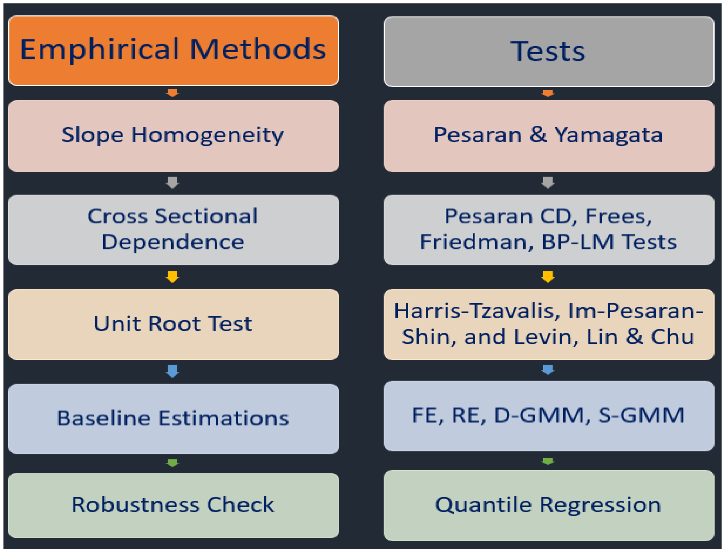
3.3. Empirical Framework

The steps followed by the empirical investigation are shown in Figure 1, where the left side is empirical methods, and the other is empirical tests. This study employs a multi-stage econometric model to examine the interplay between tourism, population, GDP, renewable energy, and electricity consumption in low-income nations, all impacting carbon emissions. To begin, a slope homogeneity test is performed to determine if there is a constant relationship between the variables across countries. This check helps ensure that the observed relationships in the data are robust and unaffected by different slopes. The next step is to conduct a cross-sectional dependence (CSD) test to look for evidence of a correlation between the data points. This test is vital because it tackles the correlation problem and enables suitable changes in the subsequent analysis to prevent biased results. According to our findings, CSD does not exist. Because countries with low incomes have limited or no linkages to one another through trade, tourism, education, religion, and treaties, we utilized unit root tests of the first generation. The Harris–Tzavalis (HT) test, Im–Pesaran–Shin (IPS) test, and Levin, Lin, and Chu (LLC) test are three of the most often used unit root tests for determining whether or not the variables are stationary. Stationarity is a prerequisite for reliable regression analysis since it eliminates the possibility of erroneous associations between the variables. The generalized method of moments (GMM) is used for estimating once stationarity has been verified. To deal with endogeneity and obtain reliable estimates, panel data analysis frequently uses GMM. The risk of error due to missing data or confounding correlations between independent factors and carbon emissions can be mitigated in this way. Quantile Regression is also used to evaluate the reliability of the findings. Using this method, we can see how the impacts of tourism, GDP, population, renewable energy, and electricity consumption vary across different levels of carbon emissions by analyzing the connections among quantiles of the dependent variable. That the results are not based merely on the mean effect but also take into account potential heterogeneity throughout the distribution of carbon emissions is what the robustness check is for. A comprehensive analysis of the impact of tourism, GDP, population, renewable energy, and electricity consumption on carbon emissions in low-income nations is the goal of this investigation, which will employ this econometric methodology at each stage. This improved knowledge of the complicated interaction between these variables is made possible using these rigorous analytic approaches, ensuring the conclusions’ reliability and validity.

3.4. Slope Homogeneity Test

Table 3. Slope homogeneity test.

Slope Homogeneity Tests	Δ Statistic	p-Value
$\check{\mathsf{\Delta }}$ test	11.674 ***	0.000
${\check{\mathsf{\Delta }}}_{\mathrm{a}\mathrm{d}\mathrm{j}}$ test	15.472 ***	0.000

The null hypothesis here is that all slope coefficients are homogeneous. Therefore, *** denotes less than 1% level.

shows the findings of a test that Levin et al. [64] did to see if all slopes were identical. Heterogeneity is a problem for the model, which should not be a surprise. This supports the idea that the parameter’s coefficients are not set, and the slope changes from country to country. Because the panel causality analysis depends on the idea that the dependent variable is the same everywhere, rejecting slope homogeneity means you should be careful before making any firm conclusions.

Equation (6) is the outcome of the slope homogeneity test:

$$\check{\mathsf{\Delta }}=\sqrt{\mathrm{N}}(\frac{{\mathrm{N}}^{-1}\mathrm{S}\mathrm{\%}-\mathrm{k}}{\sqrt{2\mathrm{k}}}) \mathrm{and} {\check{\mathsf{\Delta }}}_{\mathrm{a}\mathrm{d}\mathrm{j}}=\sqrt{\mathrm{N}}(\frac{{\mathrm{N}}^{-1}\mathrm{S}\mathrm{\%}-\mathrm{k}}{\sqrt{\frac{2\mathrm{k}(\mathrm{T}-\mathrm{k}-1)}{\mathrm{T}+1}}})$$

(6)

3.5. CSD Test

Several tests such as the Pesaran, Friedman, BP-LM, and Frees tests show cross-sectional dependence in this data set (

Table 4. Results of CSD test.

	H0: There Exists a Cross-Sectional Dependence
	Test Statistics	p-Value
Pesaran CD test	−0.601	0.5478
Frees test	2.625	Critical Value 0.3103
Friedman test	11.064	0.9953
BP LM test	8.024	0.4215

). Thus, there is a link between the different terms for making a mistake used in other countries. This is why the cross-sectional dependency-based panel unit root test and the cross-sectional reliance co-integrating analysis were used in the current research.

3.6. Unit Root Test

In panel data analysis, determining whether or not a variable is stationary is typically performed with one of three popular unit root tests: the Harris–Tzavalis (HT), Im–Pesaran–Shin (IPS), or Levin, Lin, and Chu (LLC) test. Stationarity is a necessary assumption for proper regression analysis because it guarantees that the associations between the variables are not fictitious. Harris and Tzavalis [65] presented the Harris–Tzavalis test derived from the augmented Dickey–Fuller (ADF) test statistic to address the possibility of CSD in panel data. This test compares the null hypothesis of a unit root with the alternative hypothesis of stationarity and accounts for the possibility of different unit roots in different cross-sectional units. In addition, Im, Pesaran, and Shin [66] proposed the Im–Pesaran-Shin (IPS) test, which expands on the ADF test and considers common components to solve the problem of cross-sectional dependence. It compares the alternative stationarity hypothesis with the unit root’s null hypothesis, allowing for homogeneous and heterogeneous unit root processes across the panel units. Another unit root test that considers structural breaks is the one provided by Im et al. [66]. In cases when structural changes over time might compromise the stationarity of the variables, this test comes in especially handy. Using the ADF test statistic, the LLC test compares the alternative hypothesis of stationarity with structural breakdowns with the null hypothesis of a unit root. These unit root tests shed light on the data’s stationarity qualities by revealing whether or not the variables exhibit a long-run relationship. These econometric tests allow researchers to examine the connections between tourism, population, GDP, renewable energy, electricity consumption, and carbon emissions in low-income countries in a way that considers the possibility of non-stationarity.

Table 5. Unit root test.

	At Level			At 1st Difference
Variables	Harris–Tzavalis	Im–Pesaran–Shin	Levin, Lin, and Chu	Harris–Tzavalis	Im–Pesaran–Shin	Levin, Lin, and Chu
Ln(CO2)	0.258	0.826	−0.471	−30.35 ***	−8.765 ***	−5.613 ***
Ln(TA)	1.52	2.194	4.70	−32.44 ***	−9.13 ***	−7.29 ***
Ln(POP)	−1.18	−0.636	−0.559	−31.93 ***	−9.177 ***	−7.82 ***
Ln(GDPPC)	0.911	1.045	0.362	−32.10 ***	−8.956 ***	−5.15 ***
Ln(GDPPC2)	−0.536	−0.763	−0.073	−38.19 ***	−9.33 ***	−7.88 ***
Ln(REN)	−1.18	−0.636	−0.559	−31.93 ***	−9.177 ***	−7.82 ***
Ln(AE)	−1.11	0.517	0.545	−37.52 ***	−9.769 ***	−7.72 ***

Note that, *** stand for 1% level of significance. Assume the trend and the intercept. Source: Author’s Calculation.

shows the unit roots’ results.

Panel data analysis uses the panel unit root test to determine whether the dependent and independent variables are stationary. In academic writing, you can find several panel unit root tests. Table 5 shows the unit root test results as a level or initial difference between the two variables. For example, H₀ has a unit root, but H₁ does not because it is not a stationary process. The table shows that all variables stay the same at I (1). Again, we could use the GMM and QR models.

3.7. Generalized Method of Moments (GMM)

To reach a specific study goal, different econometric approaches are used. Ln(POP) and ln(GDPPC) significantly affect CO₂ emissions, and our analytical method will make it easy to see how they are related. Our study uses it, especially the system GMM econometric approach. From 2001 to 2020, T = ten years, less than the number of cross-sections (N = 26 Countries). Roodman [67] said that the fact that crime data are constantly changing is a good strategy. Compared to earlier GMM econometric methods, the system GMM method gives more accurate and reliable results [68]. The predicted link between the standard error and the nation-fixed effects was also taken into account in our method. The problem with dynamic punitive data could be better because there is less time and more cross-sections [69]. The system GMM method can solve issues of endogeneity and heterogeneity. Because our analysis of carbon dioxide emissions is based on institutional and macroeconomic factors that are not dependent on each other, there may be a problem with reverse causality. Omri et al. [70] and Abdouli and Hammami [71] look at the reliability of a GMM system in addition to how well it deals with omitted variable bias. Blundell and Bond [72] built on a strategy that Arellano and Bond [73] and Arellano and Bover [74] had already given. The two-step GMM method makes more precise forecasts than the one-step version. Use the Hansen test [75] or the Sargan test [76] to determine how good an instrument is. On the other hand, the Sargan test is better [77]. We use the two-step Regression analysis as our primary econometric tool to examine how tourism and carbon emission are related. The use of two-step GMM is affected by the following factors:

• There are more countries in our sample (N) than years (T).
• There is a stronger connection than 0.8 between the regression model and their lateness.
• The average correlation estimator’s assumptions need help with synchronicity and variables that need to be considered.
• The two-stage GMM technique fixes biases that happen when separating variables.

Equations (7) and (8) are the traditional system-GMM and differenced-GMM Equations.

Our two-step System GMM for total international tourists’ arrivals:

$${\mathrm{L}\mathrm{n}\left({\mathrm{C}\mathrm{O}}_2\right)}_{\mathrm{i},\mathrm{t}}={\mathsf{\alpha }}_0+{\mathsf{\alpha }}_1{\mathrm{L}\mathrm{n}\left({\mathrm{C}\mathrm{O}}_2\right)}_{\mathrm{i},\mathrm{t}-\mathsf{\tau }}+{\mathsf{\alpha }}_2{\mathrm{L}\mathrm{n}\left(\mathrm{T}\mathrm{A}\right)}_{\mathrm{i},\mathrm{t}}+{\sum }_{\mathrm{k}=1}^4{Փ\Phi }_3{\mathrm{L}\mathrm{n}\left(\mathrm{X}\right)}_{\mathrm{k},\mathrm{i},\mathrm{t}-\mathsf{\tau }}+{\mathsf{\epsilon }}_{\mathrm{i},\mathrm{t}}$$

(7)

$$\begin{array}{c}\mathrm{L}\mathrm{n}{({\mathrm{C}\mathrm{O}}_2)}_{\mathrm{i},\mathrm{t}}-\mathrm{L}\mathrm{n}{({\mathrm{C}\mathrm{O}}_2)}_{\mathrm{i},\mathrm{t}-\mathsf{\tau }}={\mathsf{\alpha }}_1(\mathrm{L}\mathrm{n}{({\mathrm{C}\mathrm{O}}_2)}_{\mathrm{i},\mathrm{t}-\mathsf{\tau }}-\mathrm{L}\mathrm{n}{({\mathrm{C}\mathrm{O}}_2)}_{\mathrm{i},\mathrm{t}-2\mathsf{\tau }})+{\mathsf{\alpha }}_2({\mathrm{L}\mathrm{n}(\mathrm{T}\mathrm{A})}_{\mathrm{i},\mathrm{t}}-{\mathrm{L}\mathrm{n}(\mathrm{T}\mathrm{A})}_{\mathrm{i},\mathrm{t}-\mathsf{\tau }})+\\ \sum _{\mathrm{k}=1}^4{Փ}_3{(\mathrm{L}\mathrm{n}(\mathrm{X})}_{\mathrm{k},\mathrm{i},\mathrm{t}-\mathsf{\tau }}-\mathrm{L}\mathrm{n}{(\mathrm{X})}_{\mathrm{k},\mathrm{i},\mathrm{t}-2\mathsf{\tau }})+({\mathsf{\epsilon }}_{\mathrm{i},\mathrm{t}}-\\ {\mathsf{\epsilon }}_{\mathrm{i},\mathrm{t}-\mathsf{\tau }})\end{array}$$

(8)

CO₂ is the total carbon dioxide the country releases in year t. TA is the number of tourists from other countries who visit certain countries. The letter X stands for the number of control factors. Many tourism and environmental studies have used GMM [78,79,80,81,82].

3.8. Quantile Regression (QR)

This paper also looks at the relationship between CO₂ emissions and other relationships between the independent variable at 25%, 50%, and 75% using the QR method. Those specific quantiles are a great way to determine how much CO₂ is being put into the air. Equation (9) is the quantile model for arrivals of tourists from other countries:

$$\begin{gathered} {\mathrm{QR}}_{\mathrm{i},\mathrm{t}}={\mathsf{\alpha }}_{\mathrm{i}}^{\mathrm{q}}+{\mathsf{\beta }}_{\mathrm{i},\mathrm{Ln}\left(\mathrm{T}\mathrm{A}\right)}^{\mathrm{q}} {\mathrm{QR}}_{\mathrm{Ln}\left(\mathrm{TA}\right),\mathrm{it}}+{\mathsf{\beta }}_{\mathrm{i},\mathrm{Ln}\left(\mathrm{G}\mathrm{D}\mathrm{P}\right)}^{\mathrm{q}}{\mathrm{QR}}_{\mathrm{Ln}\left(\mathrm{GDP}\right),\mathrm{it}}+{\mathsf{\beta }}_{\mathrm{i},\mathrm{Ln}\left(\mathrm{R}\mathrm{E}\mathrm{N}\right)}^{\mathrm{q}} {\mathrm{QR}}_{\mathrm{Ln}\left(\mathrm{REN}\right),\mathrm{it}}+{\mathsf{\beta }}_{\mathrm{i},\mathrm{Ln}\left(\mathrm{A}\mathrm{E}\right)}^{\mathrm{q}} {\mathrm{QR}}_{\mathrm{Ln}\left(\mathrm{AE}\right),\mathrm{it}} \\ +{\mathsf{\beta }}_{\mathrm{i},\mathrm{Ln}\left(\mathrm{P}\mathrm{O}\mathrm{P}\right)}^{\mathrm{q}}{\mathrm{QR}}_{\mathrm{Ln}\left(\mathrm{POP}\right),\mathrm{it}} \end{gathered}$$

(9)

Numerous tourism and environmental studies have made use of quantile regression techniques [83,84,85,86,87,88,89].

4. Empirical Results and Findings

Table 6. Dynamic and static panel regression result.

Variables	FE	RE	D-GMM	S-GMM
Ln(CO2)			0.605 *** (0.0805)	0.885 *** (0.0490)
Ln(POP)	1.395 *** (0.159)	0.911 *** (0.0640)	0.628 *** (0.208)	0.138 * (0.0719)
Ln(TA)	−0.0204 (0.0217)	−0.0164 (0.0218)	−0.0256 ** (0.0123)	−0.0217 ** (0.0114)
Ln(GDPPC)	0.114 (0.194)	0.355 * (0.188)	0.510 * (0.267)	0.246 ** (0.1210)
Ln(GDPPC2)	0.0107 (0.0139)	−0.00351 (0.0138)	−0.0383 * (0.0194)	−0.0355 * (0.0183)
Ln(REN)	−0.669 *** (0.105)	−0.516 *** (0.0528)	−0.695 *** (0.261)	−0.134 *** (0.0393)
Ln(AE)	0.0618 (0.0514)	0.216 *** (0.0404)	0.0310 (0.0358)	−0.0206 (0.0409)
Constant	−13.67 *** (2.420)	−7.864 *** (1.072)	−5.678 ** (2.494)	−0.707 (1.178)
Hausman test		16.47 **
AR-1				0.007
AR-2				0.115
Hansen Test			0.571	0.780
Sargan Test			0.163	0.130
R-squared	0.582	0.5214	0.5624	0.7102
Observations	329	329	288	313
Number of ids	26

Standard errors in parentheses. *** p < 0.01, ** p < 0.05, * p < 0.1.

, presented in the analysis, examines the relationship between the dependent variable, Ln(CO₂) (natural logarithm of CO₂ emissions), and several independent variables using different econometric models such as fixed effects (FE), random effects (RE), differenced generalized method of moments (D-GMM), and system generalized method of moments (S-GMM). Regarding the impact of the variables on Ln(CO₂) emissions, the results indicate the following: Ln(POP) (natural logarithm of the population) shows consistent and significant effects across the different models. In both FE and RE models, Ln(POP) has a positive and statistically significant impact on Ln(CO₂) emissions. Similarly, D-GMM and S-GMM models also find a positive and meaningful relationship between Ln(POP) and Ln(CO₂) emissions, suggesting that population growth contributes to increased CO₂ emissions. The 1% increasing population shows 1.395% CO₂ emission in fixed effects, 0.911% CO₂ emission in random effects, 0.628% CO₂ emission in S-GMM, and 1.395% CO₂ emission in D-GMM. Ln(TA) (natural logarithm of tourism) does not exhibit consistent significance across the different models. Ln(TA) does not significantly impact Ln(CO₂) emissions in the FE and RE models. However, D-GMM and S-GMM models indicate a negative and statistically significant relationship between Ln(TA) and ln(CO₂) emissions. The coefficients are −0.020, −0.0164, −0.0256 **, and −0.0217 ** for all four models. Ln(GDPPC) (natural logarithm of GDP per capita) shows positive coefficients. In the FE model, Ln(GDPPC) does not have a statistically significant impact on Ln(CO₂) emissions. However, RE, D-GMM, and S-GMM models find a positive and statistically significant relationship between Ln(GDPPC) and Ln(CO₂) emissions. The coefficients are 0.114, 0.355 *, 0.510 *, and 0.246 ** for all four models. Ln(GDPPC²) has no statistically significant impact on Ln(CO₂) emissions in both FE and RE models.

However, D-GMM and S-GMM models find a negative and statistically significant relationship between Ln(GDPPC²) and ln(CO₂) emissions. The coefficients are −0.010, −0.0035, −0.0383 *, and −0.0355 *** for all four models. Ln(REN) (natural logarithm of renewable energy) consistently shows a negative and statistically significant impact on ln(CO₂) emissions across all models. This implies that increased renewable energy usage is associated with lower CO₂ emissions. This finding highlights the importance of promoting renewable energy sources to reduce carbon emissions. The 1% increasing renewable energy shows −0.669% CO₂ emission decreasing in fixed effects, −0.516% in random effects, −0.695% in S-GMM, and 0.134% in D-GMM. Ln(AE) (natural logarithm of electricity) does not consistently exhibit statistical significance across the models. In the RE model, Ln(AE) positively impacts Ln(CO₂₎ emissions, suggesting that higher electricity consumption is associated with increased CO₂ emissions. However, Ln(AE) does not statistically impact Ln(CO₂) emissions in the FE, D-GMM, and S-GMM models.

The regression results provide insights into the relationships between the independent variables and Ln(CO₂) emissions. These findings can be valuable for understanding the factors influencing CO₂ emissions and informing policy decisions to reduce carbon emissions and promote sustainable development.

Quantile regression results for the STRIPAT models are shown in

Table 7. Quantile regression for STRIPAT models.

Variables	Q25	Q50	Q75
Ln(POP)	0.251 * (0.128)	0.267 * (0.130)	0.322 (0.291)
Ln(TA)	−0.0190 (0.0753)	−0.0681 ** (0.0345)	−0.0283 (0.0418)
Ln(GDPPC)	0.191 ** (0.090)	0.415 ** (0.212)	0.601 * (0.319)
Ln(GDPPC2)	−0.174 *** (0.073)	−0.193 *** (0.0329)	−0.0977 *** (0.0188)
Ln(REN)	−0.328 *** (0.132)	−0.253 *** (0.111)	−0.274 *** (0.124)
Ln(AE)	0.0665 (0.101)	0.0615 (0.0592)	0.0573 (0.0558)
Observations	207	207	207

Standard errors in parentheses *** p < 0.01, ** p < 0.05, * p < 0.1. Source: Calculation by the authors.

. Ln(CO₂), which stands for carbon dioxide emissions, is the dependent variable of interest here. Q25 represents the 25th percentile, Q50 represents the median, and Q75 represents the 75th percentile, all shown as estimates in the table. This analysis will consider the following independent variables: The Ln(POP) coefficient is positive for all three quantiles, but only the Q25 coefficient is significant at the 10% level. This indicates a positive correlation between population and Ln(CO₂) emissions, especially for the bottom 25th percentile. Although the Ln(TA) coefficient changes between quantiles, the coefficient for the middle quantile is the only one with statistical significance. These data suggest that tourism significantly affects Ln(CO₂) emissions at the interquartile range. Higher GDP per capita is correlated with higher Ln(CO₂) emissions, as seen by the positive and statistically significant (at the 5% level) coefficients for Ln(GDPPC) in both Q25 and Q50. Even if the coefficient for Q75 is positive, it is not statistically significant. There is a nonlinear link between GDP per capita squared and Ln(CO₂) emissions, as seen by the negative and statistically significant coefficient for Ln(GDPPC²) across all three quantiles. The effect of GDP per capita squared on Ln(CO₂) emissions decreases as GDP per capita increases in value. All quantiles of Ln(REN) have negative coefficients, and these coefficients are statistically significant. This shows that Ln(CO₂) emissions decrease at all quantiles as renewable energy penetration increases. Quantile-wise, Ln(AE)’s coefficient fluctuates, but none of the variations are statistically significant. This suggests that the impact of electricity consumption on Ln(CO₂) emissions at various quantile levels is insignificant. These results help fill out our picture of what drives CO₂ emissions at various intensities.

5. General Discussion

Increases in carbon dioxide emissions and environmental deterioration have been linked to rapid population expansion in low-income and poor countries. Unsustainable behaviors and rising pollution are frequently the results of the expanding population’s burden on the planet’s finite resources and inadequate infrastructure. Increasing numbers of people necessitate more power, driving up consumption and growing reliance on fossil fuels, which are major sources of greenhouse gas emissions. In addition, high population growth rates are exacerbated by the lack of access to education and family planning options in many countries. To mitigate CO₂ emissions and reduce environmental degradation in these sensitive regions, it is essential to address population increase through sustainable development measures such as investments in education, healthcare, and access to family planning. The results also indicate that low-income and underdeveloped countries can benefit from increased tourism by reducing their CO₂ emissions and environmental deterioration. Investing in sustainable practices and conservation activities will help these countries’ tourism industries thrive. Improved trash management, better conservation of natural resources, and using renewable energy sources are all possible thanks to the money brought in by tourists. Moreover, tourism may educate travelers about environmental concerns, encouraging eco-friendly vacations that respect local traditions [90,91]. However, it requires meticulous planning and management to keep tourism growth aligned with sustainable principles and reduce its adverse effects on local ecosystems and communities. The results support the idea that the environmental Kuznets curve (EKC) holds even in countries with low per capita GDP. The EKC claims that the correlation between GDP per capita and environmental deterioration is “inverted U” shaped. The findings point to an initial increase in CO₂ emissions alongside rising GDP or income. This is because a growing economy often increases energy demand and industrialization. According to the analysis, CO₂ emissions and environmental degradation increase when GDP per capita squared increases. This indicates that rising GDP per capita is associated with falling CO₂ emissions after a certain economic growth point. This tipping point is when a country’s economy is strong enough to support greener technologies, stricter regulations, and more environmentally friendly policies. Therefore, the results suggest that economic growth in low-income and poor nations can lead to environmental improvement and CO₂ emissions from economic expansion decoupling when accompanied by appropriate policies and investments. Achieving sustainable development, however, calls for a delicate balancing act and all-encompassing measures that put environmental protection ahead of economic growth [92].

The results show that low-income and impoverished countries can significantly cut CO₂ emissions and environmental degradation by expanding their renewable energy consumption. Using fewer fossil fuels, a key source of greenhouse gas emissions, is possible as these countries boost their use of renewable energy sources including solar, wind, and hydroelectric power. Environmental degradation caused by carbon-intensive activities can be reduced if low-income and impoverished countries switch to cleaner energy sources. Putting money into renewable energy infrastructure has been shown to positively affect the economy, the labor market, and energy availability, all contributing to long-term sustainability. These results highlight the significance of prioritizing investments in renewable energy and establishing supportive policies in low-income and impoverished countries to obtain environmental and socioeconomic advantages. It has been found that higher CO₂ emissions and environmental degradation are linked to higher energy consumption and greater access to electricity in low-income and poor countries [93]. Several factors contribute including using fossil fuels to generate electricity, inefficient infrastructure, and a need for clean energy options. Increasing demand for power means using carbon-intensive energy sources such as coal or diesel generators. The environmental impact of electricity production may be made worse by the need for more capability for environmental legislation and sustainable energy practices. Sustainable energy transitions, promotion of renewable energy sources, and investment in cleaner technologies that minimize the carbon footprint of electricity generation in low-income and impoverished nations are critical to solving this problem.

6. Conclusions

In essence, the findings of this study provide light on how tourism, GDP, renewable energy, and electricity consumption all have a role in shaping carbon emissions in low-income countries. The results shed light on several salient points that can inform interventions in policy and sustainable development strategies. First, the analysis shows that tourism and the environment have a favorable relationship, which means that the tourism industry may help the environment in some ways. This means underdeveloped nations must prioritize encouraging environmentally friendly tourism activities that reduce their harmful impact on global warming gases. Second, the results support the environmental Kuznets curve (EKC) theory, which suggests that rising income levels in low-income nations do not automatically have adverse effects on the environment. The need to balance economic development and environmental protection must be balanced. Third, the data show that CO₂ emissions increase with GDP per capita, electrical consumption, and population. Low-income nations need better energy management and population control techniques to reduce environmental impact. This study also emphasizes the significance of using renewable energy sources to lower carbon emissions. Reducing carbon dioxide emissions and promoting sustainable development in low-income nations can benefit significantly from encouraging the adoption of renewable energy sources. Findings suggest that authorities should implement measures to increase the use of renewable energy sources, promote ecologically responsible tourism behaviors, and reduce greenhouse gas emissions. Fourth, more work needs to be performed to control population increase and curb wasteful use of the planet’s limited supplies of natural capital. In conclusion, this study reaffirms the feasibility of sustainable development in low-income nations by incorporating environmental factors into economic and tourism policy. Governments may help ensure a more sustainable and resilient future for their countries by taking preventative actions such as supporting renewable energy and sustainable tourist practices.

7. Theoretical and Practical Implications

Population growth in low-income countries is a major contributor to greenhouse gas emissions and environmental damage, which can be reduced if specific policy suggestions are implemented. First, before deciding on a family size or method of contraception, people need access to comprehensive family planning programs. Second, education and awareness campaigns about the need for environmental conservation, resource management, and sustainable practices can motivate people to act responsibly and reduce the negative effects of population growth on the environment. Third, investing in sustainable development initiatives prioritizing renewable energy sources and energy efficient technology can help decouple population growth from rising carbon emissions. Fourth, the environmental impact of a growing population on land degradation and deforestation can be mitigated, according to the fourth point, by supporting sustainable agricultural systems such as organic farming and agroforestry. Finally, stronger governance and institutions are needed to enforce environmental legislation and support sustainable development methods, which is why these recommendations are essential. Specific policy suggestions might be applied to maximize tourism’s potential as a tool for sustainable development in low-income nations. Creating and enforcing environmental norms and standards for the tourism industry is crucial to ensuring businesses use eco-friendly methods and leave a small ecological imprint. Second, community-based tourism programs that offer people a voice in policymaking and give them a stake in the outcomes can help build a more responsible and sustainable tourist business.

Thirdly, reducing carbon emissions can be aided by tourism sector investment in renewable energy infrastructure and energy efficiency services. The fourth tactic would be to promote environmentally responsible behavior among travelers and locals through public awareness and education campaigns. Lastly, encouraging partnerships and collaborations between government, tourist stakeholders, and international organizations can support low-income nations to develop and uphold sustainable tourism practices. Policy proposals for addressing the link between GDP and CO₂ emissions in low-income nations can be informed by findings supporting the environmental Kuznets curve (EKC) hypothesis. First, companies investing in green technology R&D and implementation should receive tax breaks and funding incentives. Second, a circular economy by investing more in recycling, reusing, and waste reduction initiatives to stimulate economic growth and reduce environmental damage should be promoted. Thirdly, economic expansion should be fueled while limiting environmental damage by investing in renewable energy, efficient transportation networks, and other forms of sustainable infrastructure. Promoting sustainable agricultural practices including organic farming, agroforestry, and climate-resilient farming can increase productivity while decreasing emissions. Finally, green funding frameworks and stakeholder collaboration should be established and promoted to attract sustainable investments and develop novel approaches. Developing countries can lessen their carbon footprint and boost their economies by implementing these novel solutions. Specific policy ideas might be adopted to effectively minimize CO₂ emissions and environmental deterioration to stimulate the widespread use of renewable energy in low-income nations. First, encourage the growth of microgrids that supply local communities with electricity from renewable sources such as solar, wind, and hydro. This improves local communities’ capacity to produce sustainable energy, expands access to electricity in remote places, and reduces demand for fossil fuels. Second, make it easier for individuals and organizations to launch renewable energy enterprises by providing them with support mechanisms such as training and finance. Growth, employment, and innovation in the local renewable energy sector are all boosted by this strategy. Last but not least, promote the development of energy cooperatives so that locals can combine their resources to manage and finance renewable energy projects. Off-grid renewable energy options such as solar home systems, small-scale wind turbines, and mini-hydro projects are essential for providing clean and consistent electricity access in rural and disadvantaged areas. As a final step, developing nations and international organizations should collaborate to help low-income countries adopt and integrate renewable energy technologies utilizing technology transfer and capacity-building programs. Adopting these policies can help low-income nations contribute to global climate goals and pave the way for sustainable development. In addition, the increasing CO₂ emissions and environmental damage resulting from low-income countries’ reliance on power imports and local generation can be mitigated by implementing specific policy ideas.

As a first step, we must devote significant resources to developing and deploying decentralized renewable energy sources such as solar mini-grids and home wind turbines. This approach promotes decentralized energy production, reduces reliance on fossil fuels, and enables individual communities to generate their clean electricity. Second, we must promote programs that teach people how to save energy and give them money. The adoption of energy-saving appliances, construction plans, and lighting systems should be encouraged while educating the public on energy efficiency’s economic and ecological benefits. Third, the retrofitting of existing power plants with cleaner, more efficient technology should be incentivized. It is essential to stimulate the replacement of outdated coal-fired power stations with newer ones that use cleaner fuels such as natural gas or the installation of pollution control devices. Fourthly, it is vital to encourage the introduction of novel financing vehicles such as green bonds or public-private partnerships to attract investment in renewable energy projects and upgrade the power infrastructure. Finally, developing countries must be encouraged to join international alliances and partnerships to boost their ability for technology transfer, information sharing, and institutional development.

8. Limitations and Future Research Directions

The research uses a model with an insufficient collection of variables to examine the connection between tourism, GDP, renewable energy, electricity consumption, and carbon emissions. However, the analysis may only be complete if other elements such as industrial activities, transportation emissions, and policy interventions are addressed. Furthermore, this study’s results only apply to the twenty-six low-income nations that were the focus of the investigation. Different countries’ socioeconomic and environmental conditions may prevent the generalizability of the findings. Because of this, the results should not be generalized to the entire world without further qualification. In addition, results depend on the accessibility and quality of data sources used to generate them. This study could be skewed or hindered by the availability of incomplete data or data with potential measurement mistakes or inconsistencies. Therefore, more countries and at least 50 years of data should be incorporated into future studies.

References

1. Brida, J.G.; Pulina, M.A. Literature Review on the Tourism-Led-Growth Hypothesis. Working Paper. 2010; pp. 1–26. Available online: https://crenos.unica.it/crenos/sites/default/files/WP10-17.pdf (accessed on 23 January 2023).
2. Brau, R.; Lanza, A.; Pigliaru, F. How fast are small tourism countries growing? Evidence from the data for 1980–2003. Tour. Econ. 2007, 13, 603–613. [Google Scholar] [CrossRef]
3. World Travel, Tourism Council (WTTC). 2019. Available online: https://www.wttc.org/economic-impact (accessed on 15 April 2019).
4. World Travel & Tourism Council. Travel and Tourism: Economic Impact Research Methodology 2019. Available online: https://www.wttc.org/economic-impact/country-analysis/methodology/ (accessed on 11 December 2019).
5. Chisadza, C.; Clance, M.; Gupta, R.; Wanke, P. Uncertainty and tourism in Africa. Tour. Econ. 2022, 28, 964–978. [Google Scholar] [CrossRef]
6. UNWTO. 2022. Available online: https://www.eunwto.org/doi/book/10.18111/9789284422012 (accessed on 22 September 2022).
7. World Tourism Organization (UNWTO). International Tourism Highlights, 2019, Edition. Available online: https://www.eunwto.org/doi/pdf/10.18111/9789284421152 (accessed on 4 May 2023).
8. Ehigiamusoe, K.U.; Lean, H.H.; Smyth, R. The moderating role of energy consumption in the carbon emissions-income nexus in middle-income countries. Appl. Energy 2020, 261, 114215. [Google Scholar] [CrossRef]
9. Dogan, E.; Seker, F. The influence of actual output, renewable and nonrenewable energy, trade and financial development on carbon emissions in the top renewable energy countries. Renew. Sustain. Energy Rev. 2016, 60, 1074–1085. [Google Scholar] [CrossRef]
10. Liu, A.; Wu, D.C. Tourism productivity and economic growth. Ann. Tour. Res. 2019, 76, 253–265. [Google Scholar] [CrossRef]
11. Dietz, T.; Rosa, E.A. Effects of population and affluence on CO2 Emissions. Proc. Natl. Acad. Sci. USA 1997, 94, 175–179. [Google Scholar] [CrossRef] [PubMed] [Green Version]
12. Rahman, M.H.; Voumik, L.C.; Islam, M.J.; Halim, M.A.; Esquivias, M.A. Economic Growth, Energy Mix, and Tourism-Induced EKC Hypothesis: Evidence from Top Ten Tourist Destinations. Sustainability 2022, 14, 16328. [Google Scholar] [CrossRef]
13. Arbulu, I.; Lozano, J.; Rey-Maquieira, J. Waste generation flows and tourism growth: A STIRPAT model for Mallorca. J. Ind. Ecol. 2017, 21, 272–281. [Google Scholar] [CrossRef]
14. Voumik, L.C.; Islam, M.A.; Nafi, S.M. Does tourism have an impact on carbon emissions in Asia? An application of fresh panel methodology. Environ. Dev. Sustain. 2023, 1–19. [Google Scholar] [CrossRef]
15. Shahbaz, M.; Sbia, R.; Hamdi, H.; Ozturk, I. Economic growth, electricity consumption, urbanization and environmental degradation relationship in the United Arab Emirates. Ecol. Indic. 2014, 45, 622–631. [Google Scholar] [CrossRef]
16. Shi, K.; Ren, M.; Zhitomirsky, I. Activated carbon-coated carbon nanotubes for energy storage in supercapacitors and capacitive water purification. ACS Sustain. Chem. Eng. 2014, 2, 1289–1298. [Google Scholar] [CrossRef]
17. Pao, H.T.; Tsai, C.M. Modeling and forecasting the CO2 emissions, energy consumption, and economic growth in Brazil. Energy 2011, 36, 2450–2458. [Google Scholar] [CrossRef]
18. Liddle, B. What are the carbon emissions elasticities for income and population? Bridging STIRPAT and EKC via robust heterogeneous panel estimates. Glob. Environ. Change 2015, 31, 62–73. [Google Scholar] [CrossRef] [Green Version]
19. Liu, D.; Xiao, B. Can China achieve its carbon emission peaking? A scenario analysis based on STIRPAT and system dynamics model. Ecol. Indic. 2018, 93, 647–657. [Google Scholar] [CrossRef]
20. Xie, Q.; Xu, X.; Liu, X. Is there an EKC between economic growth and smog pollution in China? New evidence from semiparametric spatial autoregressive models. J. Clean. Prod. 2019, 220, 873–883. [Google Scholar] [CrossRef]
21. Nguyen-Thanh, N.; Chin, K.H.; Nguyen, V. Does the pollution halo hypothesis exist in this “better” world? The evidence from the STIRPAT model. Environ. Sci. Pollut. Res. 2022, 29, 87082–87096. [Google Scholar] [CrossRef]
22. Voumik, L.C.; Mimi, M.B.; Raihan, A. Nexus between Urbanization, Industrialization, Natural Resources Rent, and Anthropogenic Carbon Emissions in South Asia: CS-ARDL Approach. Anthr. Sci. 2023, 2, 48–61. [Google Scholar] [CrossRef]
23. Voumik, L.C.; Rahman, M.; Akter, S. Investigating the EKC hypothesis with renewable energy, nuclear energy, and R&D for EU: Fresh panel evidence. Heliyon 2022, 8, e12447. [Google Scholar] [CrossRef]
24. Voumik, L.C.; Nafi, S.M.; Majumder, S.C.; Islam, M.A. The impact of tourism on women’s employment in South American and Caribbean countries. Int. J. Contemp. Hosp. Manag. 2023. ahead-of-print. [Google Scholar] [CrossRef]
25. Calero, C.; Turner, L.W. Regional economic development and tourism: A literature review to highlight future directions for regional tourism research. Tour. Econ. 2020, 26, 3–26. [Google Scholar] [CrossRef]
26. Adedoyin, F.F.; Bekun, F.V. Modelling the interaction between tourism, energy consumption, pollutant emissions and urbanization: Renewed evidence from panel VAR. Environ. Sci. Pollut. Res. 2020, 27, 38881–38900. [Google Scholar] [CrossRef] [PubMed]
27. Voumik, L.C.; Ridwan, M. Impact of FDI, industrialization, and education on the environment in Argentina: ARDL approach. Heliyon 2023, 9, e12872. [Google Scholar] [CrossRef]
28. Sherafatian-Jahromi, R.; Othman, M.S.; Law, S.H.; Ismail, N.W. Tourism and CO2 emissions nexus in Southeast Asia: New evidence from panel estimation. Environ. Dev. Sustain. 2017, 19, 1407–1423. [Google Scholar] [CrossRef]
29. Rahman, M.H.; Majumder, S.C. Empirical analysis of the feasible solution to mitigate the CO2 emission: Evidence from Next-11 countries. Environ. Sci. Pollut. Res. 2022, 29, 73191–73209. [Google Scholar] [CrossRef] [PubMed]
30. Voumik, L.C.; Rahman, M.H.; Nafi, S.M.; Hossain, M.A.; Ridzuan, A.R.; Mohamed Yusoff, N.Y. Modeling Sustainable Nonrenewable and Renewable Energy Based on the EKC Hypothesis for Africa’s Ten Most Popular Tourist Destinations. Sustainability 2023, 15, 4029. [Google Scholar] [CrossRef]
31. Ravinthirakumaran, K.; Ravinthirakumaran, N. Examining the relationship between tourism and CO2 emissions: Evidence from APEC region. Anatolia Int. J. Tour. Hosp. Res. 2022, 1–15. [Google Scholar] [CrossRef]
32. Shahbaz, M.; Dube, S.; Ozturk, I.; Jalil, A. Testing the Environmental Kuznets Curve Hypothesis in Portugal. Int. J. Energy Econ. Policy 2015, 5, 475–481. [Google Scholar]
33. Chang, C.P.; Dong, M.; Sui, B.; Chu, Y. Driving forces of global carbon emissions: From time-and spatial-dynamic perspectives. Econ. Model. 2019, 77, 70–80. [Google Scholar] [CrossRef]
34. Akbostancı, E.; Türüt-Aşık, S.; Tunç, G.İ. The relationship between income and environment in Turkey: Is there an environmental Kuznets curve? Energy Policy 2009, 37, 861–867. [Google Scholar] [CrossRef]
35. Churchill, S.A.; Inekwe, J.; Smyth, R.; Zhang, X. R&D intensity and carbon emissions in the G7: 1870–2014. Energy Econ. 2019, 80, 30–37. [Google Scholar]
36. Majumdar, S.; Paris, C.M. Environmental impact of urbanization, bank credits, and energy use in the UAE—A tourism-induced EKC model. Sustainability 2022, 14, 7834. [Google Scholar] [CrossRef]
37. Answer, M.K.; Alharthi, M.; Aziz, B.; Wasim, S. Impact of urbanization, economic growth, and population size on residential carbon emissions in the SAARC countries. Clean Technol. Environ. Policy 2020, 22, 923–936. [Google Scholar] [CrossRef]
38. Ikram, M.; Zhang, Q.; Sroufe, R.; Shah, S.Z.A. Towards a sustainable environment: The nexus between ISO 14001, renewable energy consumption, access to electricity, agriculture and CO2 emissions in SAARC countries. Sustain. Prod. Consum. 2020, 22, 218–230. [Google Scholar] [CrossRef]
39. Mehmood, U. Biomass energy consumption and its impacts on ecological footprints: Analyzing the role of globalization and natural resources in the framework of EKC in SAARC countries. Environ. Sci. Pollut. Res. 2022, 29, 17513–17519. [Google Scholar] [CrossRef]
40. Azam, M.; Rehman, Z.U.; Ibrahim, Y. Causal nexus in industrialization, urbanization, trade openness, and carbon emissions: Empirical evidence from OPEC economies. Environ. Dev. Sustain. 2022, 24, 13990–14010. [Google Scholar] [CrossRef]
41. Sumaira; Siddique, H.M.A. Industrialization, energy consumption, and environmental pollution: Evidence from South Asia. Environ. Sci. Pollut. Res. 2022, 30, 4094–4102. [Google Scholar] [CrossRef]
42. Cowan, W.N.; Chang, T.; Inglesi-Lotz, R.; Gupta, R. The nexus of electricity consumption, economic growth and CO2 emissions in the BRICS countries. Energy Policy 2014, 66, 359–368. [Google Scholar] [CrossRef] [Green Version]
43. Awad, A.; Warsame, M.H. The poverty-environment nexus in developing countries: Evidence from heterogeneous panel causality methods, robust to cross-sectional dependence. J. Clean. Prod. 2022, 331, 129839. [Google Scholar] [CrossRef]
44. Gao, J.; Xu, W.; Zhang, L. Tourism, economic growth, and tourism-induced EKC hypothesis: Evidence from the Mediterranean region. Empir. Econ. 2021, 60, 1507–1529. [Google Scholar] [CrossRef]
45. Koçak, E.; Ulucak, R.; Ulucak, Z.Ş. The impact of tourism developments on CO2 emissions: An advanced panel data estimation. Tour. Manag. Perspect. 2020, 33, 100611. [Google Scholar] [CrossRef]
46. Kivyiro, P.; Arminen, H. Carbon dioxide emissions, energy consumption, economic growth, and foreign direct investment: Causality analysis for Sub-Saharan Africa. Energy 2014, 74, 595–606. [Google Scholar] [CrossRef]
47. Andjarwati, T.; Panji, N.A.; Utomo, A.; Susila, L.N.; Respati, P.A.; Bon, A.T. Impact of Energy Consumption, and Economic Dynamics on Environmental Degradation in ASEAN. Int. J. Energy Econ. Policy 2020, 10, 672–678. [Google Scholar] [CrossRef]
48. Begum, R.A.; Sohag, K.; Abdullah, S.M.S.; Jaafar, M. CO2 emissions, energy consumption, economic and population growth in Malaysia. Renew. Sustain. Energy Rev. 2015, 41, 594–601. [Google Scholar] [CrossRef]
49. Ali, H.S.; Law, S.H.; Zannah, T.I. Dynamic impact of urbanization, economic growth, energy consumption, and trade openness on CO2 emissions in Nigeria. Environ. Sci. Pollut. Res. 2016, 23, 12435–12443. [Google Scholar] [CrossRef] [PubMed]
50. Hussain, M.N.; Li, Z.; Sattar, A. Effects of urbanization and nonrenewable energy on carbon emission in Africa. Environ. Sci. Pollut. Res. 2022, 29, 25078–25092. [Google Scholar] [CrossRef]
51. Voumik, L.C.; Md. Nafi, S.; Bekun, F.V.; Haseki, M.I. Modeling Energy, Education, Trade, and Tourism-Induced Environmental Kuznets Curve (EKC) Hypothesis: Evidence from the Middle East. Sustainability 2023, 15, 4919. [Google Scholar] [CrossRef]
52. Elfaki, K.E.; Khan, Z.; Kirikkaleli, D.; Khan, N. On the nexus between industrialization and carbon emissions: Evidence from ASEAN+ 3 economies. Environ. Sci. Pollut. Res. 2022, 29, 31476–31485. [Google Scholar] [CrossRef]
53. Holdren, J.P.; Ehrlich, P.R. Human Population and the Global Environment: Population growth, rising per capita material consumption, and disruptive technologies have made civilization a global ecological force. Am. Sci. 1974, 62, 282–292. Available online: https://www.jstor.org/stable/27844882 (accessed on 21 January 2023).
54. York, R.; Rosa, E.A.; Dietz, T. STIRPAT, IPAT and IMPACT: Analytic tools for unpacking the driving forces of environmental impacts. Ecol. Econ. 2003, 46, 351–365. [Google Scholar] [CrossRef]
55. Schulze, P.C. I = PBAT. Ecol. Econ. 2023, 40, 149–150. Available online: https://elibrary.ru/item.asp?id=912792 (accessed on 5 February 2023). [CrossRef]
56. Sun, X.; Zhang, H.; Ahmad, M.; Xue, C. Analysis of influencing factors of carbon emissions in resource-based cities in the Yellow River basin under carbon neutrality target. Environ. Sci. Pollut. Res. 2023, 29, 23847–23860. [Google Scholar] [CrossRef] [PubMed]
57. Huang, J.; Li, X.; Wang, Y.; Lei, H. The effect of energy patents on China’s carbon emissions: Evidence from the STIRPAT model. Technol. Forecast. Soc. Change 2021, 173, 121110. [Google Scholar] [CrossRef]
58. Li, B.; Liu, X.; Li, Z. Using the STIRPAT model to explore the factors driving regional CO2 emissions: A case of Tianjin, China. Nat. Hazards 2021, 76, 1667–1685. [Google Scholar] [CrossRef]
59. Wang, P.; Wu, W.; Zhu, B.; Wei, Y. Examining the impact factors of energy-related CO2 emissions using the STIRPAT model in Guangdong Province, China. Appl. Energy 2021, 106, 65–71. [Google Scholar] [CrossRef]
60. De Vita, G.; Katircioglu, S.; Altinay, L.; Fethi, S.; Mercan, M. Revisiting the environmental Kuznets curve hypothesis in a tourism development context. Environ. Sci. Pollut. Res. 2015, 22, 16652–16663. [Google Scholar] [CrossRef] [PubMed]
61. Fethi, S.; Senyucel, E. The role of tourism development on CO2 emission reduction in an extended version of the environmental Kuznets curve: Evidence from top 50 tourist destination countries. Environ. Dev. Sustain. 2015, 23, 1499–1524. [Google Scholar] [CrossRef]
62. Katircioglu, S. Investigating the role of oil prices in the conventional EKC model: Evidence from Turkey. Asian Econ. Financ. Rev. 2015, 7, 498–508. [Google Scholar] [CrossRef] [Green Version]
63. Lee, J.W.; Brahmasrene, T. Investigating the influence of tourism on economic growth and carbon emissions: Evidence from panel analysis of the European Union. Tour. Manag. 2015, 38, 69–76. [Google Scholar] [CrossRef]
64. Levin, A.; Lin, C.F.; Chu, C.S.J. Unit root tests in panel data: Asymptotic and finite-sample properties. J. Econom. 2002, 108, 1–24. [Google Scholar] [CrossRef]
65. Harris, R.D.; Tzavalis, E. Inference for unit roots in dynamic panels where the time dimension is fixed. J. Econom. 1999, 91, 201–226. [Google Scholar] [CrossRef]
66. Im, K.S.; Pesaran, M.H.; Shin, Y. Testing for unit roots in heterogeneous panels. J. Econom. 2003, 115, 53–74. [Google Scholar] [CrossRef]
67. Roodman, D. How to do xtabond2: An introduction to difference and system GMM in Stata. State J. 2009, 9, 86–136. [Google Scholar] [CrossRef] [Green Version]
68. Fingleton, B. A generalized method of moments estimator for a spatial panel model with an endogenous spatial lag and spatial moving average errors. Spat. Econ. Anal. 2008, 3, 27–44. [Google Scholar] [CrossRef] [Green Version]
69. Nickell, S. Biases in dynamic models with fixed effects. Econom. J. Econom. Soc. 1981, 49, 1417–1426. [Google Scholar] [CrossRef]
70. Omri, A.; Nguyen, D.K.; Rault, C. Causal interactions between CO2 emissions, FDI, and economic growth: Evidence from dynamic simultaneous-equation models. Econ. Model. 2014, 42, 382–389. [Google Scholar] [CrossRef] [Green Version]
71. Abdouli, M.; Hammami, S. Investigating the causality links between environmental quality, foreign direct investment and economic growth in MENA countries. Int. Bus. Rev. 2017, 26, 264–278. [Google Scholar] [CrossRef]
72. Blundell, R.; Bond, S. Initial conditions and moment restrictions in dynamic panel data models. J. Econom. 1998, 87, 115–143. [Google Scholar] [CrossRef] [Green Version]
73. Arellano, M.; Bond, S. Some tests of specification for panel data: Monte Carlo evidence and an application to employment equations. Rev. Econ. Stud. 1991, 58, 277–297. [Google Scholar] [CrossRef] [Green Version]
74. Arellano, M.; Bover, O. Another look at the instrumental variable estimation of error-components models. J. Econom. 1995, 68, 29–51. [Google Scholar] [CrossRef] [Green Version]
75. Hansen, L.P.; Singleton, K.J. Generalized instrumental variables estimation of nonlinear rational expectations models. Econom. J. Econom. Soc. 1982, 50, 1269–1286. [Google Scholar] [CrossRef]
76. Sargan, J.D. The estimation of economic relationships using instrumental Variables. Econom. J. Econom. Soc. 1958, 26, 393–415. [Google Scholar] [CrossRef]
77. Iqbal, N.; Daly, V. Rent seeking opportunities and economic growth in transitional Economies. Econ. Model. 2014, 37, 16–22. [Google Scholar] [CrossRef]
78. Ozturk, I.; Al-Mulali, U.; Saboori, B. Investigating the environmental Kuznets curve hypothesis: The role of tourism and ecological footprint. Environ. Sci. Pollut. Res. 2016, 23, 1916–1928. [Google Scholar] [CrossRef] [PubMed]
79. Konstantakopoulou, I. Does health quality affect tourism? Evidence from system GMM estimates. Econ. Anal. Policy 2022, 73, 425–440. [Google Scholar] [CrossRef]
80. Musa, M.S.; Jelilov, G.; Iorember, P.T.; Usman, O. Effects of tourism, financial development, and renewable energy on environmental performance in EU-28: Does institutional quality matter? Environ. Sci. Pollut. Res. 2021, 28, 53328–53339. [Google Scholar] [CrossRef]
81. Usman, O.; Elsalih, O.; Koshadh, O. Environmental performance and tourism development in EU-28 Countries: The role of institutional quality. Curr. Issues Tour. 2020, 23, 2103–2108. [Google Scholar] [CrossRef]
82. Ferdaus, J.; Appiah, B.K.; Majumder, S.C.; Martial, A.A.A. A Panel Dynamic Analysis on Energy Consumption, Energy Prices and Economic Growth in Next 11 Countries. Int. J. Energy Econ. Policy 2020, 10, 87–99. [Google Scholar] [CrossRef]
83. Wei, L.; Ullah, S. International tourism, digital infrastructure, and CO2 emissions: Fresh evidence from panel quantile regression approach. Environ. Sci. Pollut. Res. 2022, 29, 36273–36280. [Google Scholar] [CrossRef]
84. Aziz, N.; Mihardjo, L.W.; Sharif, A.; Jermsittiparsert, K. The role of tourism and renewable energy in testing the environmental Kuznets curve in the BRICS countries: Fresh evidence from methods of moments quantile regression. Environ. Sci. Pollut. Res. 2020, 27, 39427–39441. [Google Scholar] [CrossRef]
85. Porto, N.; Ciaschi, M. Reformulating the tourism-extended environmental Kuznets curve: A quantile regression analysis under environmental legal conditions. Tour. Econ. 2021, 27, 991–1014. [Google Scholar] [CrossRef]
86. Lasisi, T.T.; Eluwole, K.K.; Alola, U.V.; Aldieri, L.; Vinci, C.P.; Alola, A.A. Do tourism activities and urbanization drive material consumption in the OECD countries? A quantile regression approach. Sustainability 2021, 13, 7742. [Google Scholar] [CrossRef]
87. Rahman, M.H.; Majumder, S.C.; Barman, S.D. Examine the Role of Agriculture to Mitigate the CO2 Emission in Bangladesh. Asian J. Agric. Rural Dev. 2020, 10, 392–405. [Google Scholar] [CrossRef]
88. Majumder, S.C.; Rahman, M.H. Rural–urban migration and its impact on environment and health: Evidence from Cumilla City Corporation, Bangladesh. GeoJournal 2022, 87, 1–19. [Google Scholar] [CrossRef]
89. Voumik, L.C.; Hossain, M.S.; Islam, M.A.; Rahaman, A. Power Generation Sources and Carbon Dioxide Emissions in BRICS Countries: Static and Dynamic Panel Regression. Strateg. Plan. Energy Environ. 2022, 41, 401–424. [Google Scholar] [CrossRef]
90. Majumder, S.C.; Voumik, L.C.; Rahman, M.H.; Rahman, M.M.; Hossain, M.N. A Quantile Regression Analysis of the Impact of Electricity Production Sources on CO2 Emission in South Asian Countries. Strateg. Plan. Energy Environ. 2023, 31, 307–330. [Google Scholar] [CrossRef]
91. Voumik, L.C.; Sultana, R.; Dey, R. Going Away or Getting Green in BRICS: Investigating the EKC Hypothesis with Human Capital Index, Nuclear Energy, Urbanization, and Service Sectors on the Environment. World Dev. Sustain. 2023, 2, 100060. [Google Scholar] [CrossRef]
92. Raihan, A.; Ibrahim, S.; Muhtasim, D.A. Dynamic impacts of economic growth, energy use, tourism, and agricultural productivity on carbon dioxide emissions in Egypt. World Dev. Sustain. 2023, 2, 100059. [Google Scholar] [CrossRef]
93. Polcyn, J.; Voumik, L.C.; Ridwan, M.; Ray, S.; Vovk, V. Evaluating the Influences of Health Expenditure, Energy Consumption, and Environmental Pollution on Life Expectancy in Asia. Int. J. Environ. Res. Public Health 2023, 20, 4000. [Google Scholar] [CrossRef]
Figure 1. Empirical Steps for the Study.
Energies 16 04608 g001