
Large Eddy Simulation of Rotationally Induced Ingress and Egress around an Axial Seal between Rotor and Stator Disks
Abstract
:1. Introduction
2. Problem Description
3. Problem Formulation
4. Numerical Method of Solution
5. Results and Discussion
5.1. Verification and Validation
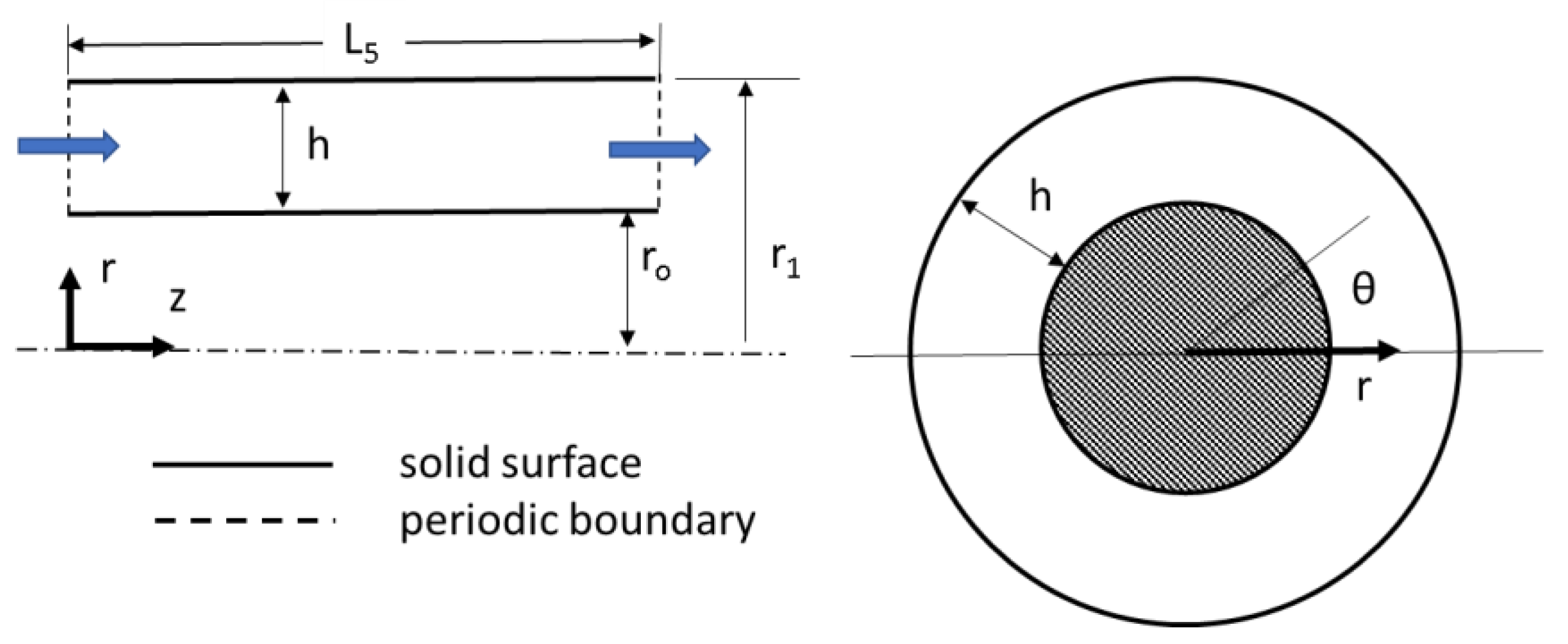
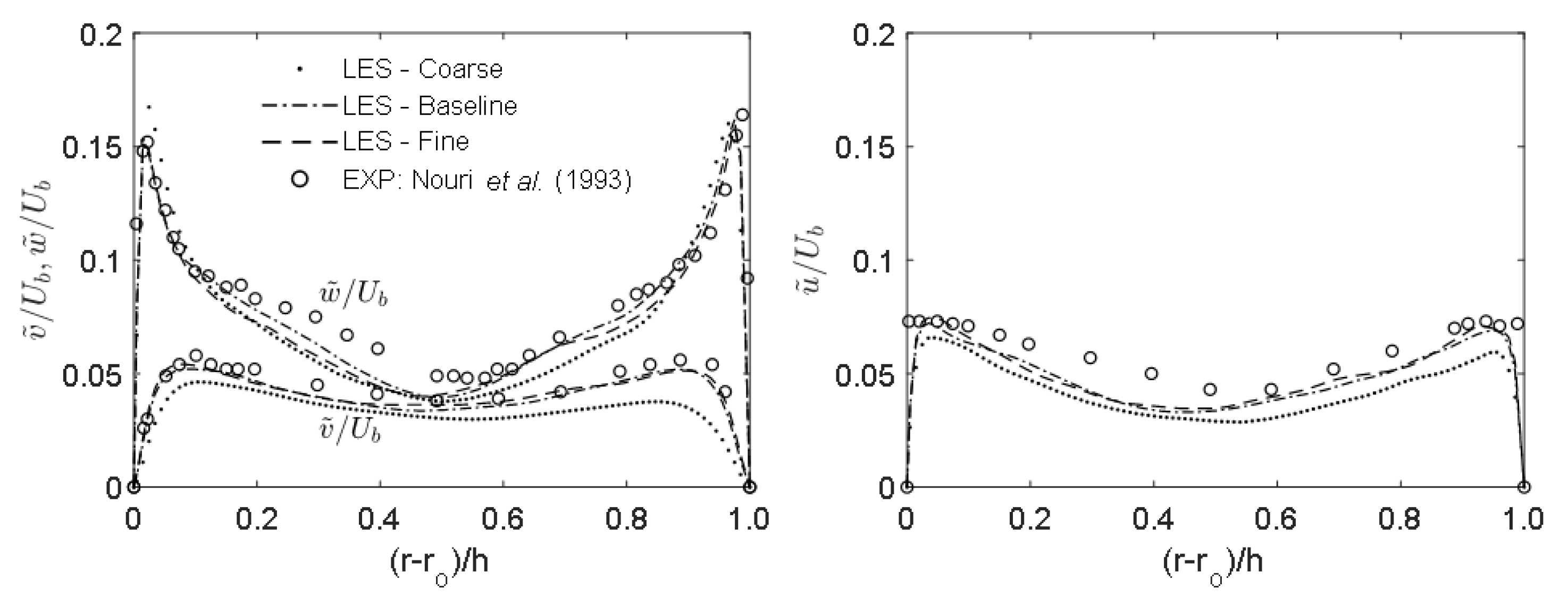
5.1.1. Fully Developed Flow in an Annulus
5.1.2. Rotor–Stator Configuration with Axial Seal
5.1.3. Effects of Inlet Turbulence and Velocity Profile on Flow in Seal
5.2. Flow Field Induced by Rotor and Its Rotation
5.2.1. Instantaneous Flow Field
5.2.2. Time-Averaged Flow Field
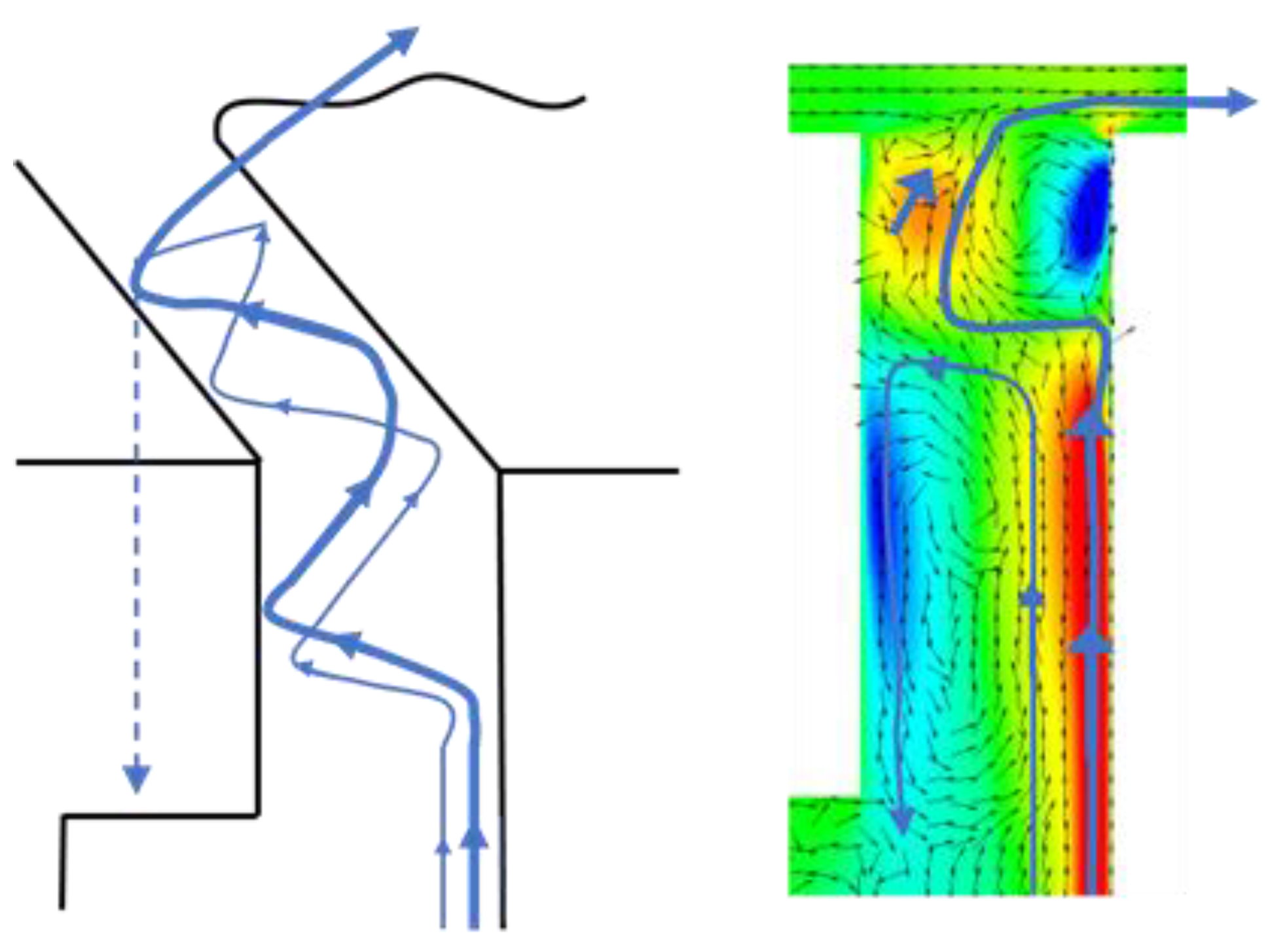
5.2.3. Mean Trajectories of Ingress and Egress
6. Summary and Conclusions
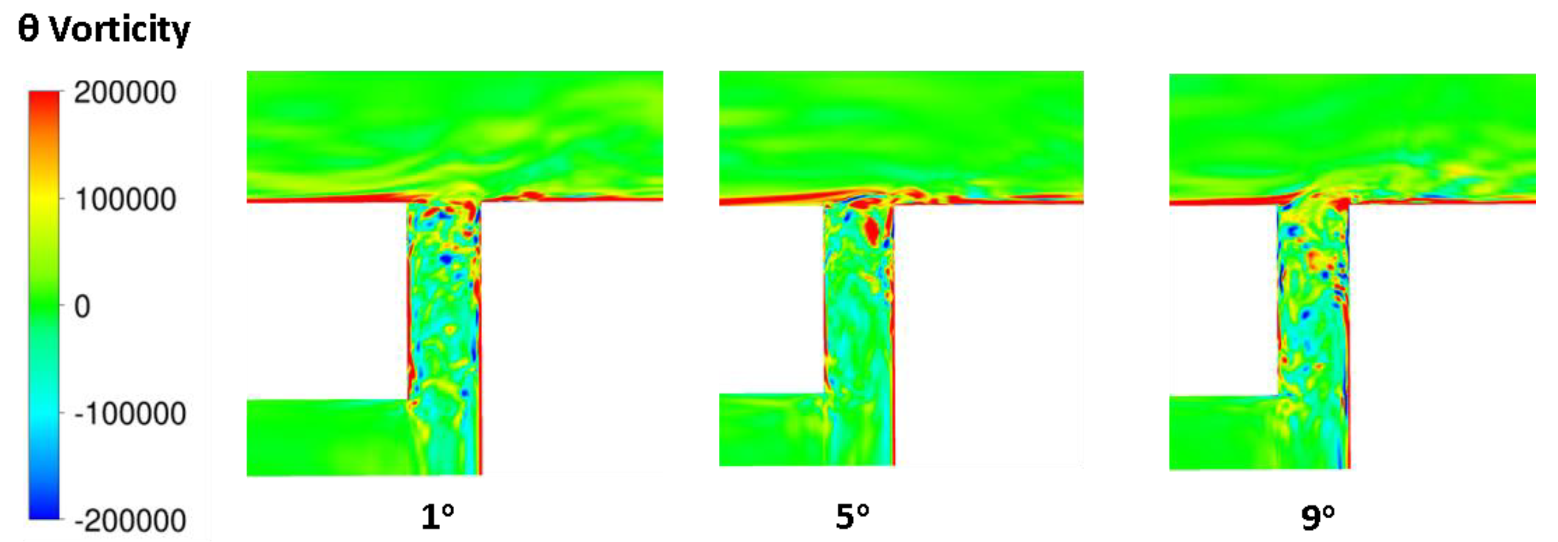
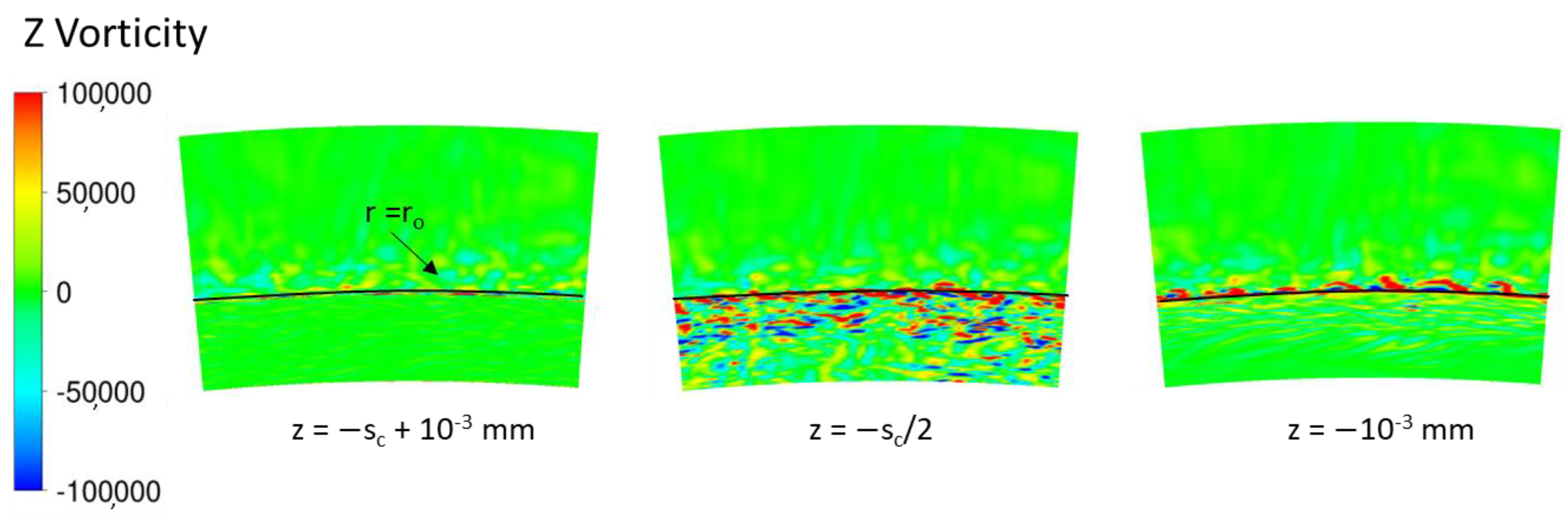
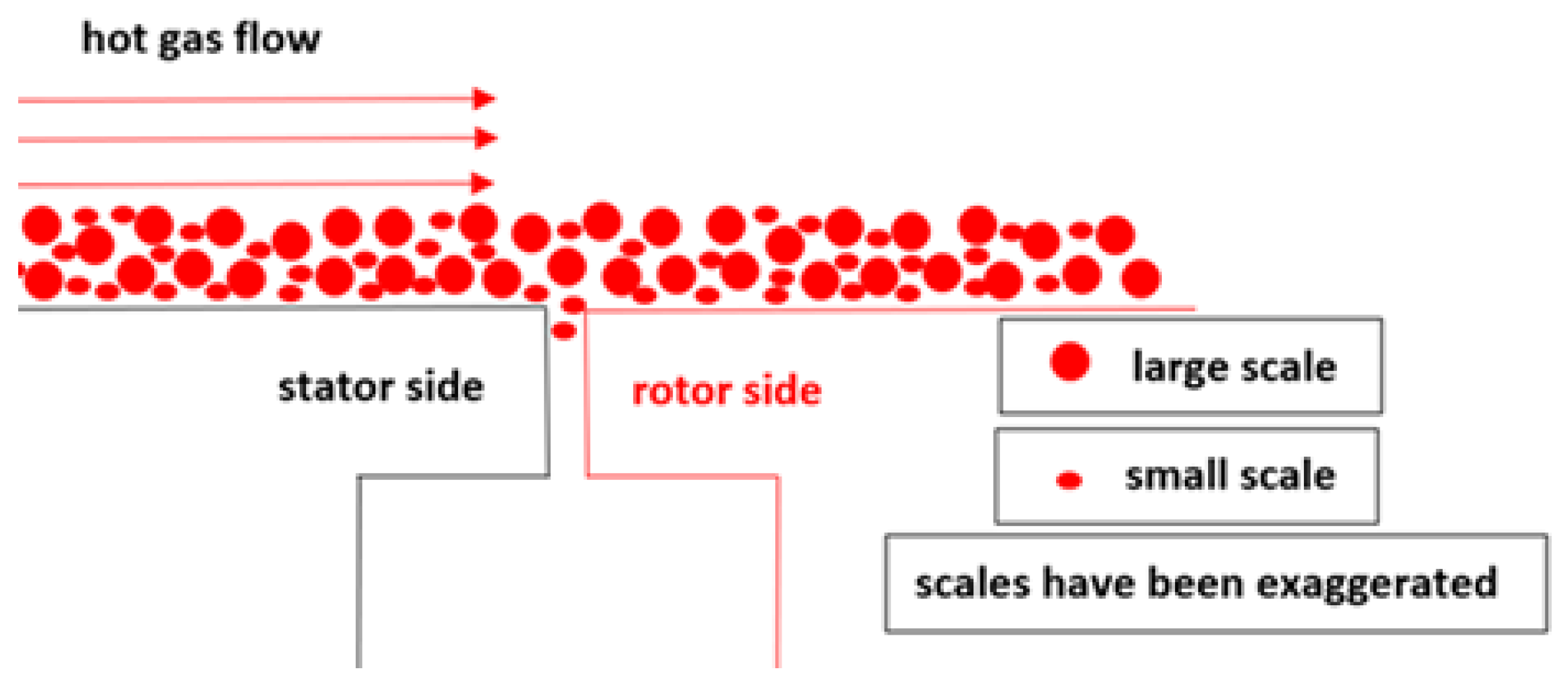
- Interaction between the hot gas flow in the axial direction and the boundary-layer flow in the azimuthal direction induced by the rotating rotor causes Kelvin–Helmholtz instability (KHI) to occur.
- The KHI forms a wavy boundary layer in the azimuthal direction with a corresponding wavy displacement thickness.
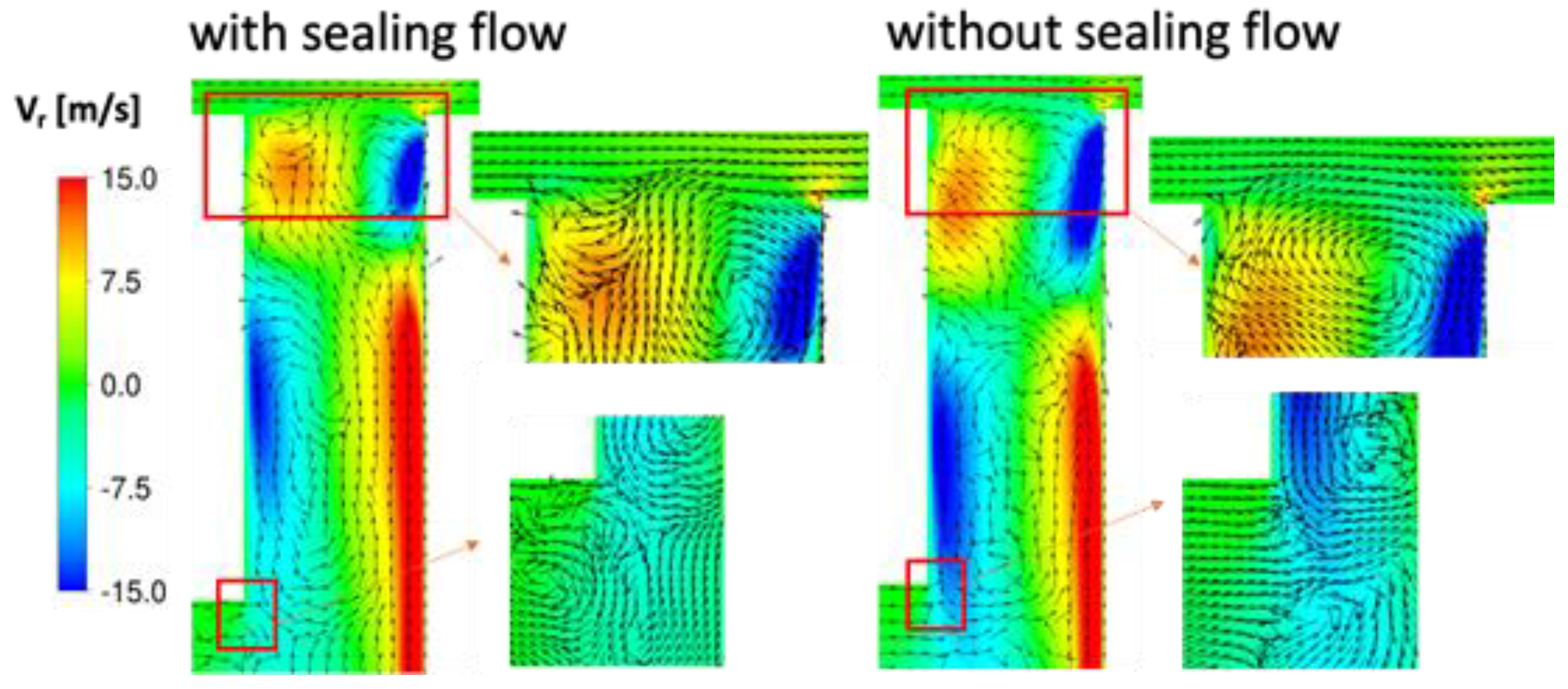
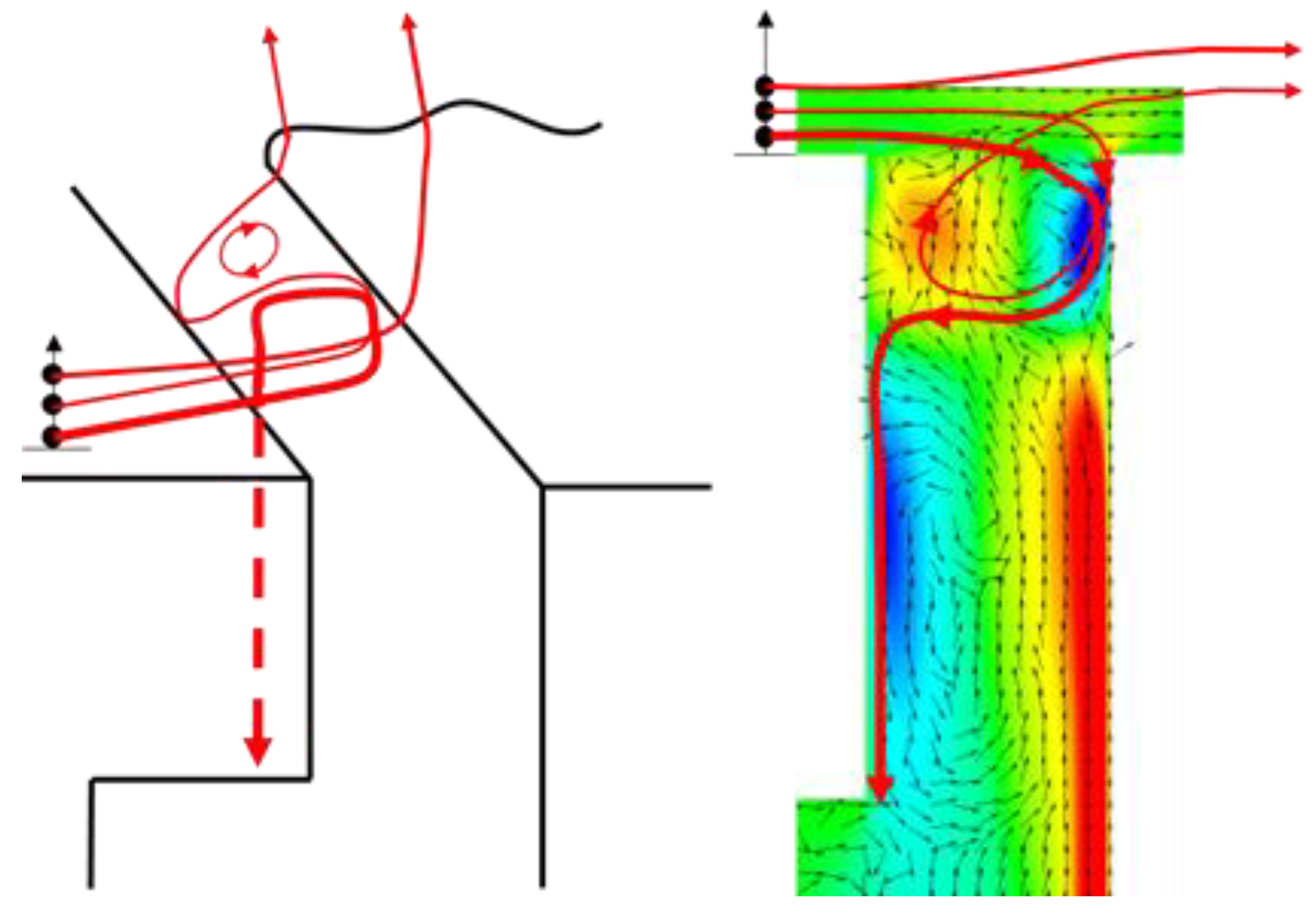
- Hot gas flow over the seal induces a series of recirculating flows in the seal clearance and causes vortex shedding at the seal’s backward-facing step.
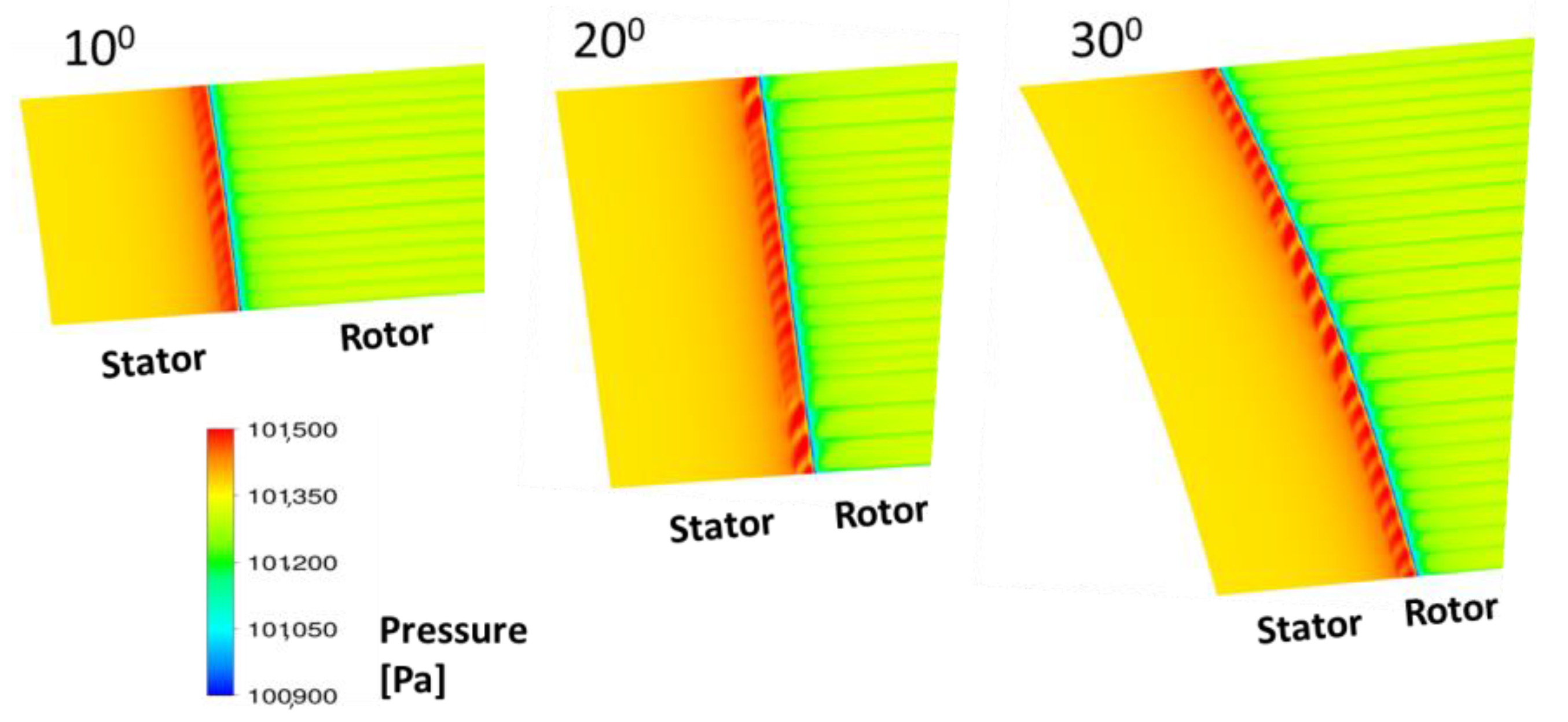
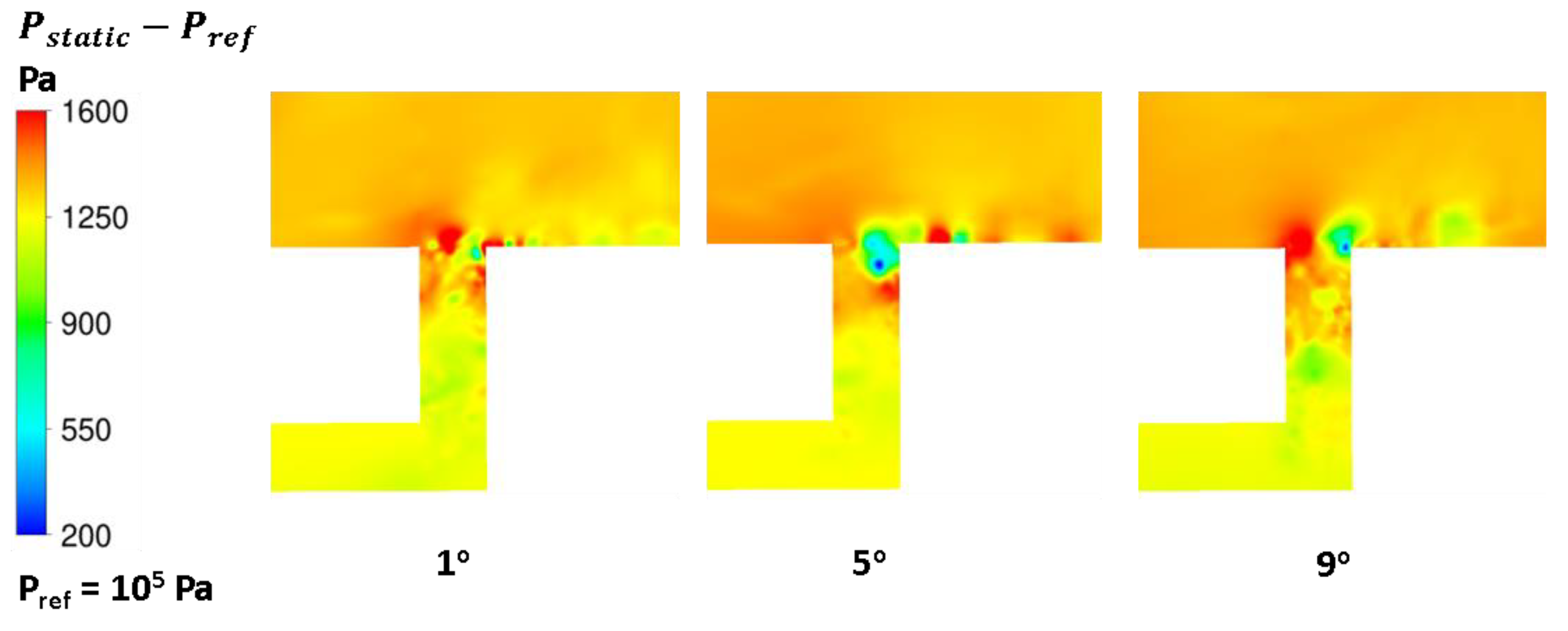
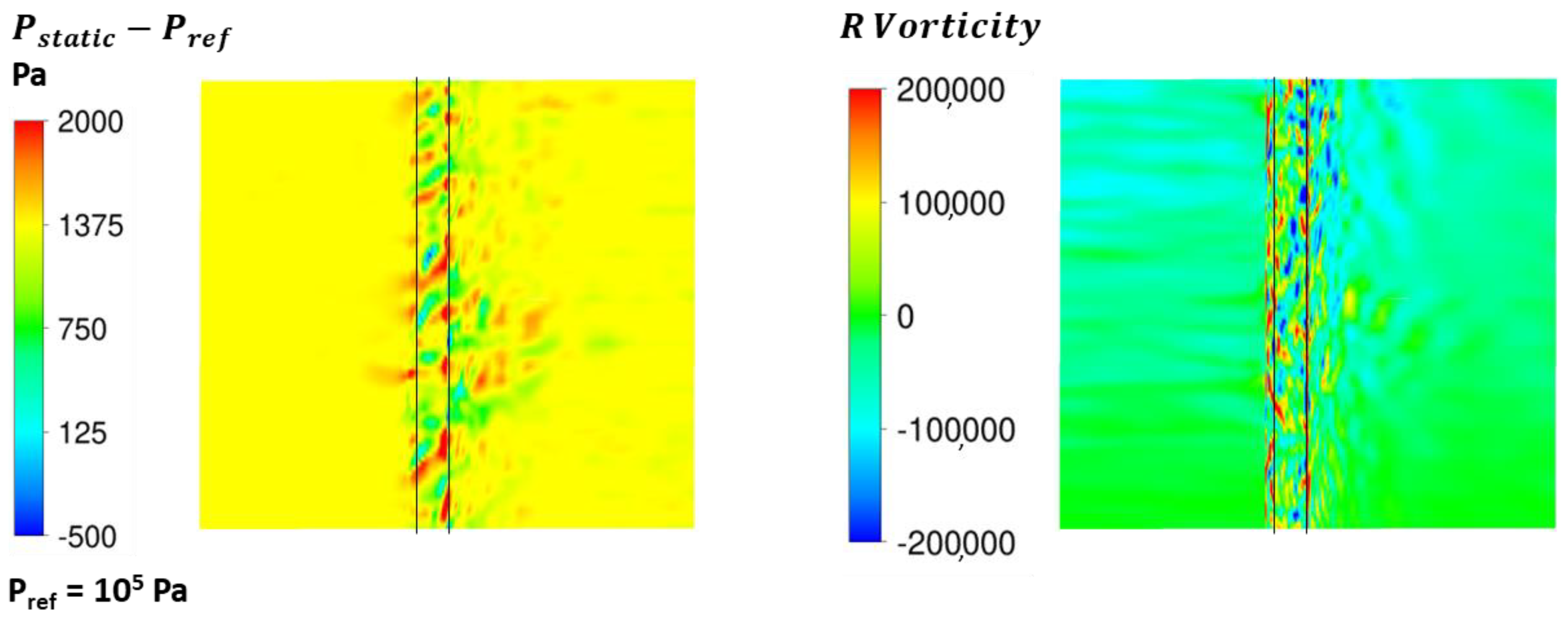
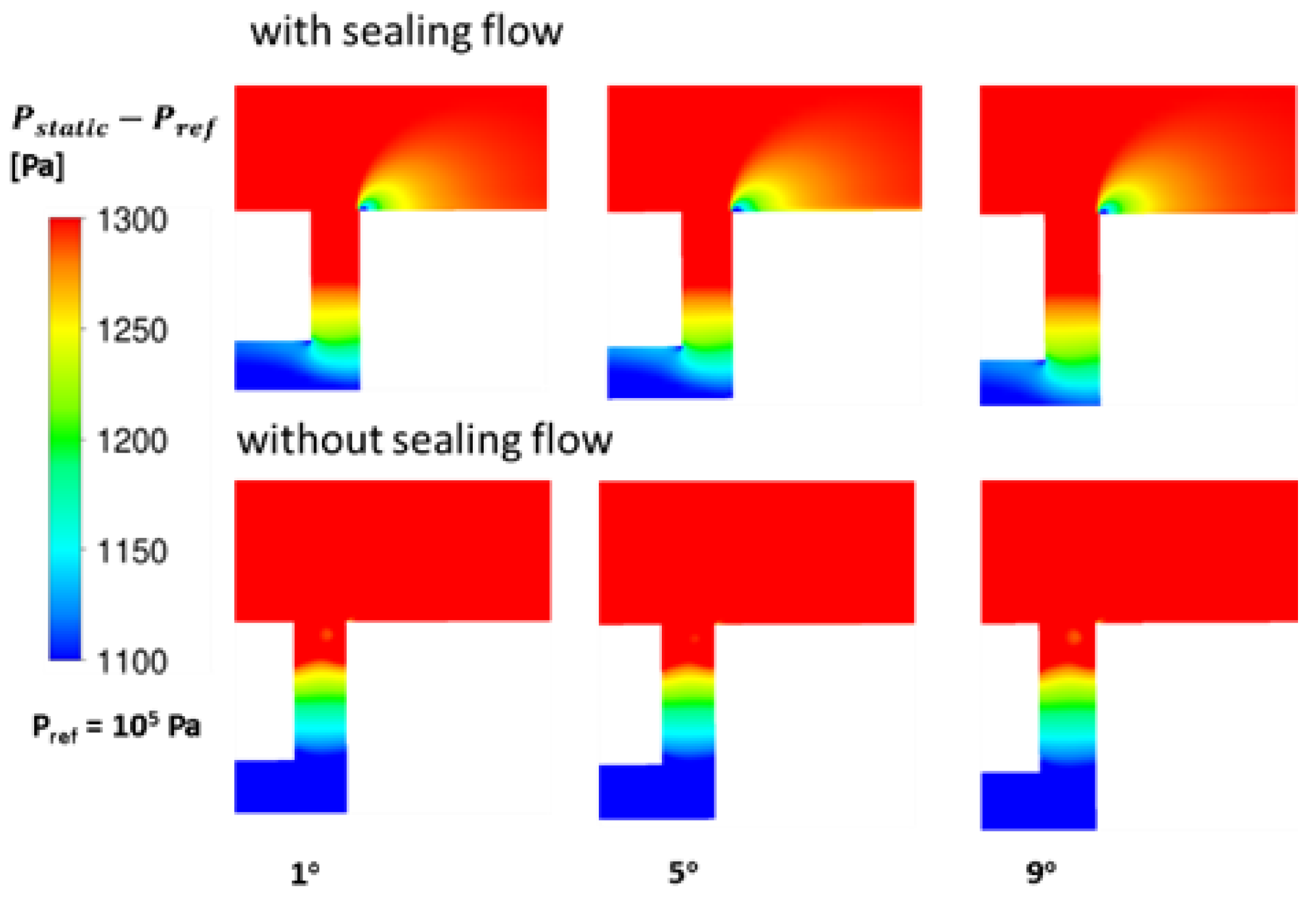
- The wavy displacement thickness formed by KHI and the impingement of shed vortices on the rotor side of the seal create alternating regions of high and low pressures around the rotor side of the seal.
- The alternating regions of high and low pressures cause ingress to start on the rotor side of the seal.
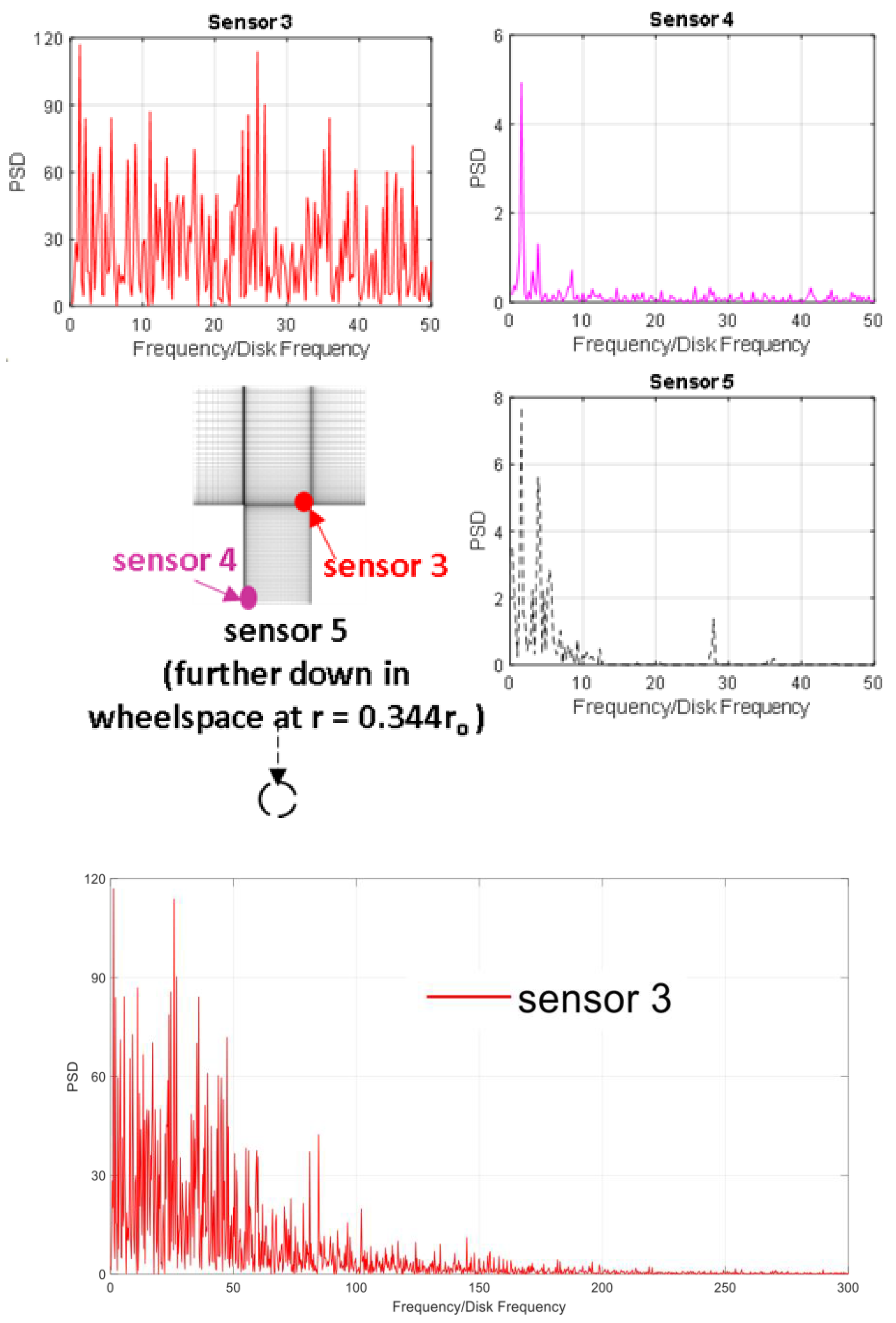
- Regions of high and low pressures around the rotor side of the seal were found to be statistically stationary and do not rotate with the rotor.
- Not all hot gases ingested into the seal reach the wheelspace because the motion induced by the spiraling recirculating flow entrains them back out into the hot gas path.
- On egress, it starts on the rotor side because of “disk pumping” in the wheelspace. However, once reaching the clearance of the seal, it becomes entrained by the recirculating flows there and exits from the stator side.
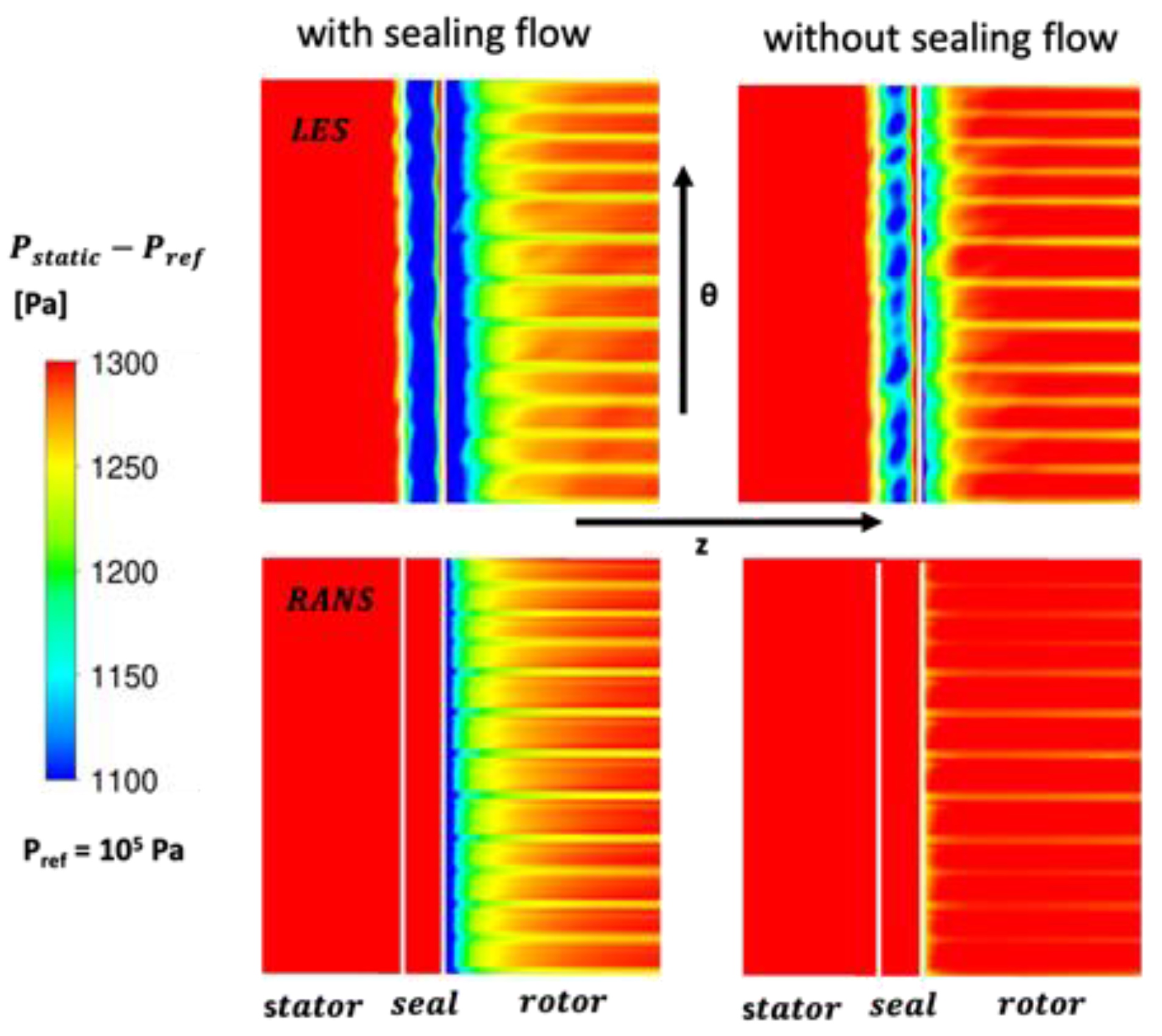
- Though RANS with the SST model was able to predict regions of high and low pressures around the rotor side of the seal, it was unable to predict ingress. LES coupled with the WALE model could predict regions of high and low pressures around the rotor side of the seal and the ingress that they create.
Author Contributions
Funding
Conflicts of Interest
Nomenclature
| nondimensional coolant flow rate: | |
| Dh | hydraulic diameter |
| G | gap ratio |
| Gc | clearance ratio |
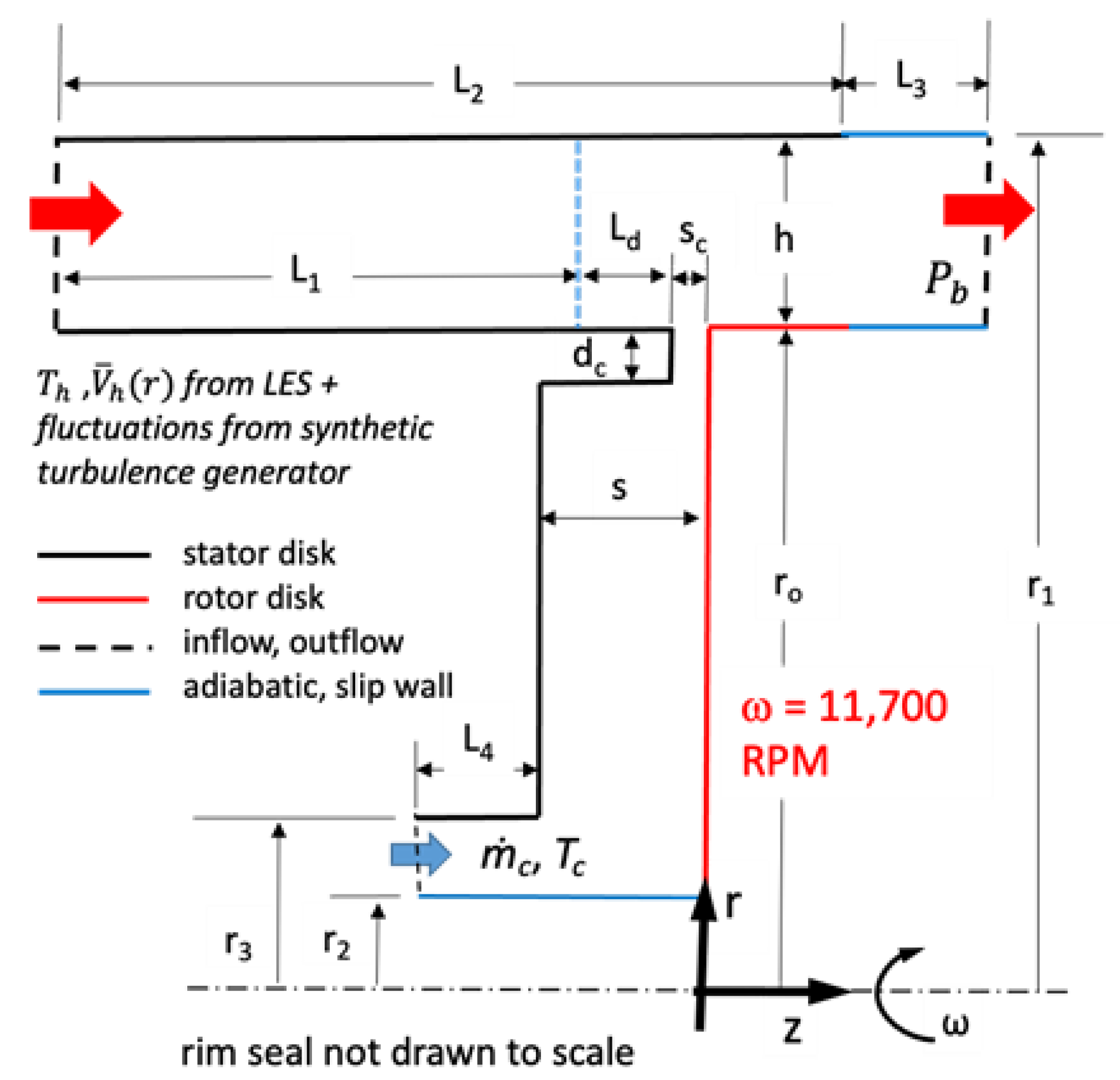
| H | height of annulus (see Figure 3 and Figure 4) |
| I | turbulence intensity |
| Li | length (i = 1, 2, 3, 4, 5; see Figure 3 and Figure 4) |
| ṁ | mass flow rate |
| P | pressure |
| Pb | back pressure |
| r | radial coordinate |
| ro | radius of hub/inner radius of annulus |
| r1 | outer radius of annulus |
| Reynolds number in a duct: | |
| external flow Reynolds number: | |
| rotational Reynolds number: | |
| s | axial distance between rotor and stator (gap) |
| sc | axial distance in seal opening (clearance) |
| T | temperature |
| rms of tangential velocity fluctuation in annular duct | |
| U | time-average axial velocity in annular duct |
| Ub | average bulk velocity magnitude in a duct |
| friction velocity: , where is the “local” wall shear stress | |
| rms of radial velocity fluctuation in annular duct | |
| axial-radial-velocity cross-correlation | |
| V | velocity |
| rms of axial velocity fluctuation in annular duct | |
| y+ | nondimensional turbulent distance |
| z | axial coordinate |
| curvature parameter: | |
| δ | boundary layer thickness |
| ε | rate of turbulence dissipation |
| θ | azimuthal coordinate |
| dynamic viscosity | |
| kinematic viscosity | |
| effective turbulent kinematic viscosity | |
| ρ | density |
| Kolmogorov time scale: | |
| normalized grid spacing: where | |
| ω | angular speed of rotor disk |
| Subscripts | |
| c | coolant flow |
| h | mainstream flow |
References
- Han, J.-C. Advanced Cooling in Gas Turbines 2016 Max Jakob Memorial Award Paper. ASME. J. Heat Transf. 2018, 140, 113001. [Google Scholar] [CrossRef]
- Goldstein, R.J.; Chen, H.P. Film Cooling on a Gas Turbine Blade Near the End Wall. J. Eng. Gas Turbines Power 1985, 107, 117–122. [Google Scholar] [CrossRef]
- Tin, S.; Pollock, T.M. Nickel-Base Superalloys in Advanced Turbine Engines. In Turbine Aerodynamics, Heat Transfer, Materials, and Mechanics; Shih, T.I.-P., Yang, V., Eds.; AIAA Progress Series; American Institute of Aeronautics and Astronautics: Washington, DC, USA, 2014; Volume 243. [Google Scholar]
- Choi, S.; Choi, S.; Cho, H. Effect of Various Coolant Mass Flow Rates on Sealing Effectiveness of Turbine Blade Rim Seal at First Stage Gas Turbine Experimental Facility. Energies 2020, 13, 4105. [Google Scholar] [CrossRef]
- Owen, J.M.; Phadke, U.P. An Investigation of Ingress for a Simple Shrouded Rotating Disc System with a Radial Outflow of Coolant. In Proceedings of the ASME 1980 International Gas Turbine Conference and Products Show, New Orleans, LA, USA, 10–13 March 1980; Volume 1A: General. [Google Scholar] [CrossRef]
- Phadke, U.P.; Owen, J.M. An Investigation of Ingress for an “Air-Cooled” Shrouded Rotating Disk System with Radial-Clearance Seals. J. Eng. Power 1983, 105, 178–182. [Google Scholar] [CrossRef]
- Phadke, U.P.; Owen, J.M. Aerodynamic Aspects of the Sealing of Gas-Turbine Rotor-Stator Systems. Part 1: The Behavior of Simple Shrouded Rotating-Disk Systems in a Quiescent Environment. Int. J. Heat Fluid Flow 1988, 9, 98–105. [Google Scholar] [CrossRef]
- Phadke, U.P.; Owen, J.M. Aerodynamic Aspects of the Sealing of Gas-Turbine Rotor-Stator Systems. Part 2: The Performance of Simple Seals in a Quasi-Axisymmetric External Flow. Int. J. Heat Fluid Flow 1988, 9, 106–112. [Google Scholar] [CrossRef]
- Phadke, U.P.; Owen, J.M. Aerodynamic Aspects of the Sealing of Gas-Turbine Rotor-Stator Systems. Part 3: The Effect of Nonaxisymmetric External Flow on Seal Performance. Int. J. Heat Fluid Flow 1988, 9, 113–117. [Google Scholar] [CrossRef]
- Sangan, C.M.; Pountney, O.J.; Zhou, K.; Owen, J.M.; Wilson, M.; Lock, G.D. Experimental Measurements of Ingestion Through Turbine Rim Seals—Part II: Rotationally Induced Ingress. J. Turbomach. 2013, 135, 021013. [Google Scholar] [CrossRef]
- Dadkhah, S.; Turner, A.B.; Chew, J.W. Performance of Radial Clearance Rim Seals in Upstream and Downstream Rotor–Stator Wheelspaces. J. Turbomach. 1992, 114, 439–445. [Google Scholar] [CrossRef]
- Bohn, D.; Johann, E.; Krüger, U. Experimental and Numerical Investigations of Aerodynamic Aspects of Hot Gas Ingestion in Rotor-Stator Systems with Superimposed Cooling Mass Flow. In Proceedings of the ASME 1995 International Gas Turbine and Aeroengine Congress and Exposition, Houston, TX, USA, 5 June 1995; Volume 1: Turbomachinery. [Google Scholar] [CrossRef]
- Cao, C.; Chew, J.W.; Millington, P.R.; Hogg, S.I. Interaction of Rim Seal and Annulus Flows in an Axial Flow Turbine. J. Eng. Gas Turbines Power 2004, 126, 786–793. [Google Scholar] [CrossRef]
- Boudet, J.; Autef, V.; Chew, J.; Hills, N.; Gentilhomme, O. Numerical Simulation of Rim Seal Flows in Axial Turbines. Aeronaut. J. 2005, 109, 373–383. [Google Scholar] [CrossRef]
- Jakoby, R.; Zierer, T.; Lindblad, K.; Larsson, J.; deVito, L.; Bohn, D.; Funcke, J.; Decker, A. Numerical Simulation of the Unsteady Flow Field in an Axial Gas Turbine Rim Seal Configuration. In Proceedings of the ASME Turbo Expo 2004: Power for Land, Sea, and Air, Vienna, Austria, 14–17 June 2004; Volume 4: Turbo Expo 2004, pp. 431–440. [Google Scholar] [CrossRef]
- Rabs, M.; Benra, F.-K.; Dohmen, H.J.; Schneider, O. Investigation of Flow Instabilities Near the Rim Cavity of a 1.5 Stage Gas Turbine. In Proceedings of the ASME Turbo Expo 2009: Power for Land, Sea, and Air, Orlando, FL, USA, 8–12 June 2009; Volume 3: Heat Transfer, Parts A and B, pp. 1263–1272. [Google Scholar] [CrossRef]
- Gao, F.; Chew, J.; Beard, P.; Amirante, D.; Hills, N. Large-Eddy Simulation of Unsteady Turbine Rim Sealing Flows. Int. J. Heat Fluid Flow 2018, 70, 160–170. [Google Scholar] [CrossRef]
- Liu, J.; Weaver, A.; Shih, T.I.-P.; Sangan, C.M.; Lock, G.D. Modelling and Simulation of Ingress into the Rim Seal and Wheelspace of a Gas-Turbine Rotor-Stator Configuration. In Proceedings of the 53rd AIAA Aerospace Sciences Meeting, Kissimmee, FL, USA, 5–9 January 2015. [Google Scholar] [CrossRef]
- Menter, F.R. Zonal Two-Equation k-ω Turbulence Models for Aerodynamic Flows. In Proceedings of the 23rd Fluid Dynamics, Plasmadynamics, and Lasers Conference, Orlando, FL, USA, 6–9 July 1993. [Google Scholar]
- Nicoud, F.; Ducros, F. Subgrid-Scale Stress Modelling Based on the Square of the Velocity Gradient Tensor. Flow Turbul. Combust. 1999, 62, 183–200. [Google Scholar] [CrossRef]
- Dhamankar, N.; Blaisdell, G.; Lyrintzis, A. Overview of Turbulent Inflow Boundary Conditions for Large-Eddy Simulations. AIAA J. 2018, 56, 1317–1334. [Google Scholar] [CrossRef]
- Available online: https://www.ansys.com/products/fluids/ansys-fluent (accessed on 22 May 2023).
- Patankar, S.V. Numerical Heat Transfer and Fluid Flow; Hemisphere Publishing Corp.: Washington, DC, USA, 1980. [Google Scholar]
- Nouri, J.; Umur, H.; Whitelaw, J. Flow of Newtonian and non-Newtonian Fluids in Concentric and Eccentric Annuli. J. Fluid Mech. 1993, 253, 617–641. [Google Scholar] [CrossRef]
- Quadrio, M.; Luchini, P. Direct Numerical Simulation of the Turbulent Flow in a Pipe with Annular Cross-section. Eur. J. Mech. B/Fluids 2002, 21, 413–427. [Google Scholar] [CrossRef]
- Kim, J.; Moin, P.; Moser, R. Turbulence Statistics in Fully Developed Channel Flow at Low Reynolds Number. J. Fluid Mech. 1987, 177, 133–166. [Google Scholar] [CrossRef]
- Celik, I.B.; Cehreli, Z.N.; Yavuz, I. Index of Resolution Quality for Large Eddy Simulations. J. Fluids Eng. 2005, 127, 949–958. [Google Scholar] [CrossRef]
- Schädler, R.; Kalfas, A.I.; Abhari, R.S.; Schmid, G.; Voelker, S. Modulation and Radial Migration of Turbine Hub Cavity Modes by the Rim Seal Purge Flow. J. Turbomach. 2017, 139, 011011. [Google Scholar] [CrossRef]


Disclaimer/Publisher’s Note: The statements, opinions and data contained in all publications are solely those of the individual author(s) and contributor(s) and not of MDPI and/or the editor(s). MDPI and/or the editor(s) disclaim responsibility for any injury to people or property resulting from any ideas, methods, instructions or products referred to in the content. |
© 2023 by the authors. Licensee MDPI, Basel, Switzerland. This article is an open access article distributed under the terms and conditions of the Creative Commons Attribution (CC BY) license (https://creativecommons.org/licenses/by/4.0/).
Share and Cite
Nketia, S.; Shih, T.I.-P.; Bryden, K.; Dalton, R.; Dennis, R.A. Large Eddy Simulation of Rotationally Induced Ingress and Egress around an Axial Seal between Rotor and Stator Disks. Energies 2023, 16, 4354. https://doi.org/10.3390/en16114354
Nketia S, Shih TI-P, Bryden K, Dalton R, Dennis RA. Large Eddy Simulation of Rotationally Induced Ingress and Egress around an Axial Seal between Rotor and Stator Disks. Energies. 2023; 16(11):4354. https://doi.org/10.3390/en16114354
Chicago/Turabian StyleNketia, Sabina, Tom I-P. Shih, Kenneth Bryden, Richard Dalton, and Richard A. Dennis. 2023. "Large Eddy Simulation of Rotationally Induced Ingress and Egress around an Axial Seal between Rotor and Stator Disks" Energies 16, no. 11: 4354. https://doi.org/10.3390/en16114354