Article

A Bi-Level Optimal Operation Model for Small-Scale Active Distribution Networks Considering the Coupling Fluctuation of Spot Electricity Prices and Renewable Energy Sources

1
Power Economic Research Institute of Jilin Electric Power Co., Ltd., Changchun 130021, China
2
School of Economics and Management, North China Electric Power University, Beijing 102206, China
3
Beijing Key Laboratory of New Energy and Low-Carbon Development, North China Electric Power University, Beijing 102206, China
*
Author to whom correspondence should be addressed.
Energies 2023, 16(11), 4507; https://doi.org/10.3390/en16114507
Submission received: 1 May 2023 / Revised: 25 May 2023 / Accepted: 30 May 2023 / Published: 3 June 2023
(This article belongs to the Section A: Sustainable Energy)

Abstract

:
As the penetration rate of variable renewable energy such as wind power increases in the power system, the composition and balance of the system also change gradually. The intermittency of renewable energy poses great stability challenges to the traditional centralized generation and load-oriented transmission and distribution methods. Therefore, the Active Distribution Network Operator (ADNO) with distributed installation at the local level has a good application prospect in the new scenario. However, ADNO needs to improve its operational efficiency based on the types of local generation and storage devices and the nature of the market environment. To address this issue, this paper proposes a forecasting method that considers the coupling fluctuations of spot electricity prices and renewable energy, and a bi-level optimization operation method based on the Stackelberg game for optimizing the operation of small-scale ADNO under high wind power penetration rate. Simulation results show that the proposed methods achieve greater positive impact on the operational efficiency of ADNO than conventional methods. In addition, the proposed methods ensure the long-term profitability of ADNO, even with fluctuations in external factors.

1. Introduction

In order to solve the problem of carbon emissions caused by fossil fuel power generation, energy diversification has become an important trend in power generation. Countries have put forward their own energy diversification development plans. Among them, the active distribution network is a promising energy supply model. The so-called active distribution network refers to an intelligent power system that can achieve bidirectional flow of electricity, while having energy storage, small-scale power generation units, and other functions through intelligent control technology.
The potential of active distribution networks in terms of ensuring energy security and reducing carbon emissions has been widely recognized. According to data from the International Energy Agency, by 2030, over 130 million households and businesses worldwide will use active distribution networks [1]. Countries and regions such as China, the European Union, and the United States have issued relevant policies and plans to actively promote the construction of active distribution networks.
The potential of active distribution networks in ensuring energy security and reducing carbon emissions include the following aspects:
  • It can achieve precise control of electricity through intelligent control technology, improve energy utilization efficiency, and reduce energy waste;
  • It has energy storage capacity, which can balance the load of power grid effectively and enhance the stability of the power grid;
  • Through the use of small-scale power generation units, it can better adapt to the demand for decentralized energy supply and improve the flexibility of energy supply.
Small-scale active distribution networks refer to a new type of power system that integrates distributed power sources, load control, and energy storage systems on a smaller scale based on distribution networks, forming a power system that can actively respond to the needs of the power grid. Small-scale active distribution networks have many advantages and will become an important part of future power supply systems. Small-scale active distribution networks are usually based on distribution networks with ten to dozens of nodes. They are characterized by a small scale but a very large potential base, so their market potential is also enormous. This power system can not only improve the reliability and efficiency of power supply, but also provide more services to customers. Therefore, small-scale active distribution networks have great significance for the future development of the energy field and the flexibility and low-carbon contribution of power supply systems. During peak periods of power supply, a large number of small-scale active distribution networks can quickly respond to power demand, balance the load of the power grid, and thereby improve the reliability of the power supply system. At the same time, small-scale active distribution networks promote the use of renewable energy, reduce carbon emissions, and contribute to the low-carbon development of the power system.
Nevertheless, operators of small-scale active distribution networks also face many problems. The main problems include the following three points:
  • It is difficult to influence the wholesale market price. Small-scale active distribution networks need to import electricity from the electricity wholesale market and distribute it to their customers. As price takers, operators of small-scale active distribution networks passively face price fluctuations;
  • Small-scale active distribution networks rely on controllable fossil energy or unpredictable renewable energy to provide part of their electricity internally to increase power supply flexibility. The uncertainty of variational renewable energy generation from internal and external sources can affect profitability;
  • There exists a game relationship between operators and internal customers. The strategy determined unilaterally by the operator may deviate from the equilibrium point.
This paper aims to tackle these problems through a novel conditional forecasting method and a novel bi-level optimization method. We verify the advantages of the proposed method over conventional methods in improving the operational efficiency of small-scale active distribution networks through simulation experiments, and analyze the impact of external factor fluctuations on the long-term revenue of ADNOs. This paper has important theoretical and practical value for understanding and improving the operational mechanism of small-scale active distribution networks in the context of low-carbon transformation. The rest of this paper is organized as follows: Section 2 is a literature review. The conditional forecasting method is established in Section 3. The bi-level optimization model is established in Section 4. Section 5 is a case study. The conclusions are provided in Section 6.

2. Literature Review

Active distribution networks (ADNs) are becoming increasingly important due to the integration of distributed generation, which changes power flow from unidirectional to bi-directional. In order to manage distribution networks effectively, an active network management strategy that incorporates emerging techniques of control, monitoring, protection, and communication is needed. The advantages of active distribution networks include improved operating economics and reliability of power systems and increased low-carbon performance. Several articles have explored various aspects of active distribution networks. Zhao et al. [1] provided a short review of recent advancements and identify emerging technologies and future development trends for support the active management of distribution networks. Flexible Low-Carbon Optimal Dispatch of Honeycombed Active Distribution Network (HADN) is proposed by Xiang et al. [2] as a way to increase low-carbon benefits through appropriate HADN dispatch. Ge et al. [3] proposed a substation planning method that accounts for the widespread introduction of distributed generators in a low-carbon economy. Li et al. [4] studied a bi-level interactive optimization model for active distribution networks with microgrids, which minimizes operation cost and voltage deviation to achieve a low-carbon system. Finally, Xiao et al. [5] proposed a new Distribution Management System (DMS) framework based on security region, which aims to help operate the system close to its security boundary in order to improve the efficiency significantly within the same security standard.
To maintain the optimal operation of a network, extensive research studies have been conducted under the theme of network management. Usman et al. [6] investigated losses management strategies in active distribution networks and provided a concise yet comprehensive comparison of the most recently proposed losses management approaches and strategies. Gabash and Li [7] proposed a combined problem formulation for active-reactive optimal power flow in distribution networks with embedded wind generation and battery storage. Cortes et al. [8] proposed an iterative procedure for the optimal design of a microgrid topology in active distribution networks, which applies graph partitioning, integer programming, and a performance index for the optimal design. Kyriakou and Kanellos [9] proposed a method for the coordinated optimal operation scheduling of active distribution networks that are hosting complex microgrids comprising large building prosumers and plug-in electric vehicle aggregators. Sedghi et al. [10] presented a paper on storage scheduling for optimal energy management in active distribution networks considering uncertainties of load, wind, and plug-in electric vehicles. Jiang et al. [11] proposed a combined modeling and optimal scheduling method for active distribution networks with integrated smart buildings. Chen et al. [12] proposed a stochastic optimal operation strategy for distribution networks whose objective function considers the operation state of the distribution network. In order to enhance system resilience, Wang et al. [13] proposed a novel optimal operation strategy for an active distribution network. For the issue of optimal pricing between ADNOs, Tostado-Véliz et al. [14] proposed an equilibrium problem with an equilibrium constraints (EPECs) approach, which solves the bi-level problem associated to each participant sequentially using diagonalization. Finally, Fan et al. [15] proposed a Lyapunov optimization-based online distributed (LOOD) algorithmic framework for active distribution networks (ADNs).
Active distribution networks (ADNs) are developing rapidly due to the increasing penetration of distributed energy resources (DERs), such as renewable energy sources and electric vehicles. Therefore, forecasting is essential for network management to maintain the optimal operation of ADNs. This paragraph summarizes recent research on forecasting in ADNs. Saint-Pierre and Mancarella [16] proposed a scheduling model for active distribution system management (ADSM) to operate distribution network assets with renewable energy sources. The model considers uncertainties, market constraints, and scheduled power flows at the interface with the transmission system. The proposed ADSM approach maximizes renewable penetration, minimizes deviations from time-ahead schedules, and estimates the required level of local reserves from dispatchable generation and electrical energy storage (EES) while accounting for uncertainties. Shen et al. [17] presented a planning model for ADN that considers long-term investment costs and short-term operation conditions with EES benefits for peak load shaving and power reliability enhancement. Yu et al. [18] proposed a novel spatial-temporal graph representation method to characterize and present spatial and temporal correlations of historical load observations. The graph data are used to train a model denoted as Spatial-Temporal Synchronous Graph Convolutional Network (STSGCN) that can forecast load by learning from the graph features. Kalantar-Neyestanaki et al. [19] presented a method to determine the capability area of an ADN for the provision of both active and reactive power reserves while considering forecast errors and operational constraints of the grid and DERs. Cheng et al. [20] proposed a state estimation method for ADNs based on the forecasting of photovoltaic (PV) power generation using the Gaussian mixture model (GMM). Cong et al. [21] proposed a day-ahead active power scheduling method that considers REG forecast errors to minimize distribution company costs and achieve optimal power flow with a hierarchical coordination optimization model based on chance constrained programming.
Overall, recent research has shown that forecasting plays a crucial role in the optimal operation of ADNs. Various methods, such as branch flow model-based relaxed optimal power flow [22], dual-horizon rolling scheduling models [23], and state estimation methods based on PV power generation forecasting, have been proposed to achieve optimal scheduling of active power and enhance the reliability and efficiency of ADNs. However, one might neglect the effects of the correlation between the fluctuation of wholesale spot price and the output of renewable energy. Moreover, one might overlook the function of ADNO time-of-use subsidy and the game relationship between ADNOs and users. This paper shows that with proper handling of these factors, ADNO may achieve significant profitability increase.

3. Conditional Wholesale Power Price Forecast for High VRE Penetration Market

3.1. Correlation between Wind Power Output and Electricity Spot Price in High Penetration Markets

The Active Distribution Network Operator (ADNO) needs to purchase electricity from the electricity spot wholesale market and sell it to retail customers. ADNO needs to decide on the dispatch strategy for the second day in advance. When the spot wholesale price is too high, ADNO should use appropriate advance dispatching to replace some of the external electricity supply with internal resources, such as renewable energy generators, fossil fuel generators, and energy storage equipment. Conversely, when the spot wholesale price is low, ADNO should optimize its dispatch strategy to maximize the utilization of cheap electricity from the external power grid. The basic operating model of ADNO is shown in Figure 1.
For small-scale ADNOs, due to their small scale, they cannot affect market prices and can be regarded as price takers in the spot wholesale market. Therefore, they cannot increase their profitability by influencing market prices. Therefore, accurate prediction of market prices is very important to improve their profitability.
On the other hand, appropriate renewable energy installed capacity is meaningful for reducing the operating costs of ADNOs. Variational renewable energy generation, such as photovoltaic and wind power, has very low variable costs. However, variable renewable energy (VRE) has strong intermittency and requires additional controllable distributed fuel units to supplement it, forming a power source combination. The operating sequence of ADNO is shown in Figure 2.
The power generation system is undergoing a trend of low-carbonization, which means more and more large-scale VRE power generation companies are entering the wholesale market. As a result, the power spot price is increasingly affected by VRE output. In the actual market operation, the wholesale market operator Independent System Operator (ISO) will provide a day-ahead VRE output forecast based on the information of the entire system.
For ADNOs located at a certain node of the system, they face uncertainties from three parts: VRE output, spot market price, and user load. For ADNOs in a high VRE penetration power wholesale market, the first two sources may be correlated. Ignoring this correlation may lead to a decrease in accuracy of prediction.
This article suggests that ADNOs can use the network-wide VRE output published by ISO as a condition to predict the local VRE output and node electricity prices. This can significantly improve the accuracy of predictions.
Based on dataset [24], this study calculated the correlation between VRE generation and spot prices. The dataset is from ENTSO-e and consists of time-series data of wind power generation and spot market prices in the DK market for one year. This paper first standardized the data using the formula:
x t , n o r = x t X 2
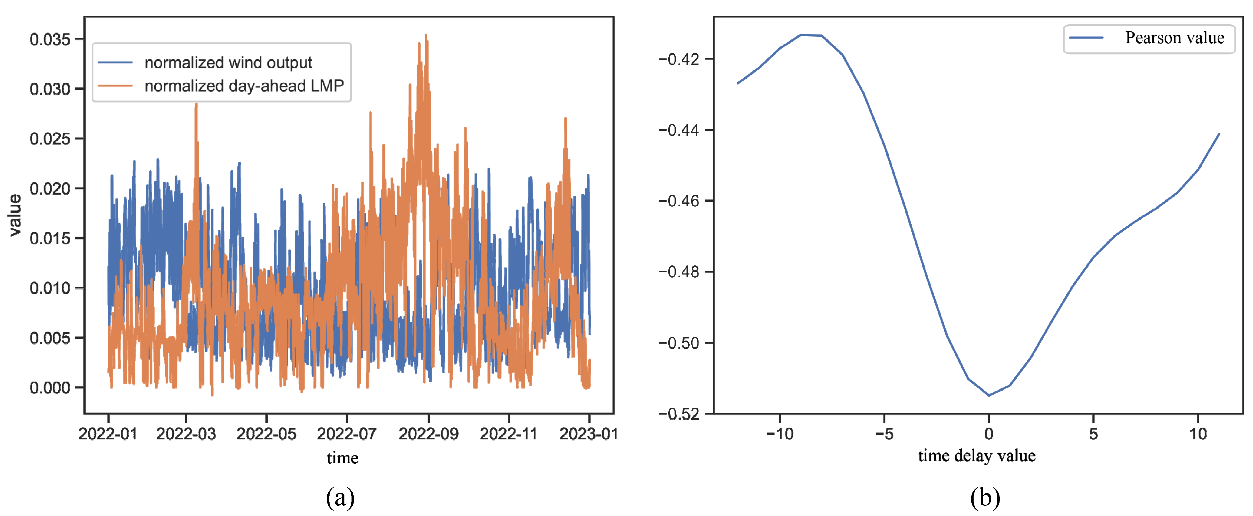
where X 2 = t x t 2 , x t is the value at time t in the time series, and X refers to the entire time series. x t , n o r is the standardized value of x t . The normalized value of wind output and day-ahead LMP are depicted in Figure 3a. This paper examined the correlation between the two time series, by calculating the Pearson correlation coefficient at different lag steps. The calculation method is as follows:
ρ W , P , N = c o v X W N , X P σ W N , σ P
where c o v X W N , X P = t x t N , W , n o r x t N , W , n o r x P x t , P , n o r . Here, X W N represents the time series of wind power generated N steps earlier, and X P represents the time series of spot prices. c o v X W N , X P is the covariance between X W N and X P . x t , , n o r is the standardized variable of wind power generation time series, and x t , , n o r is the mean of x t , n o r . σ is the standard deviation of X , calculated as σ = t x t , , n o r x t , , n o r 2 .
The time interval of the data used in this paper is 15 min. When N takes values between −10 and 10, the variation in ρ W , P , N is shown in Figure 3b. It can be seen that wind power generation and spot prices have significant negative correlation (less than −0.5) when N = 0.

3.2. ADNO Local Wind Power Output and Nodal Price Prediction Based on ISO Wind Power Forecast

3.2.1. Improved Transformer Time Series Conditional Prediction Model

This study constructs a prediction model based on the principle of Bayesian inference. As shown in Section 3.1, the local nodal electricity price of ADNO and the wind power output forecast of ISO are highly correlated under high penetration rates. Therefore, we built a conditional prediction model, which we apply to the prediction of ADNO local wind power output and nodal prices separately.
This paper constructs a prediction model based on the principle of maximizing the conditional likelihood probability, as shown in Formula (3).
p x y N , θ = t = t 0 T 1 p x t + 1 x t 0 , x t , y t 0 N , , y t N , θ
where N is the time delay step that maximizes the Pearson correlation between the two time series x and y . This paper constructs a parameter model to map this conditional probability, and the value of the parameter θ should be the value that maximizes p x y , θ , that is,
θ * = a r g m a x θ p ( x y N , θ )
Regarding the selection of the prediction parameter model, there are linear models and nonlinear models. Recent studies have shown that nonlinear models represented by deep neural networks have achieved good results in many complex conditional prediction tasks [25,26,27]. In deep neural networks, there are various options for such prediction tasks based on autoregressive networks (such as LSTM, GRU, etc.) and convolutional networks (such as WaveNet) [28]. Considering the specificity of this prediction task, this study adopts the transformer network for prediction. Multiple studies have shown that transformer networks can model longer time spans and often achieve better results in price prediction tasks than autoregressive networks and convolutional networks.
This paper uses the transformer [29] deep neural network for conditional prediction. It improved the structure of the original transformer to make it more suitable for the prediction task of this study. The basic structure is shown in Figure 4.
First, this study adjusts the input and output structure of the transformer. It first performs mean–variance standardization on all sequences to make them stationary and ensure that their values are in the range [−1, 1]. Then, it outputs the predicted mean and variance, rather than the probability of a specific category.

3.2.2. Multi-Head Attention Mechanism

The multi-head attention mechanism in the transformer is a mechanism that can simultaneously focus on different parts of the input sequence. The transformer uses the positional encoding module [29] to handle the temporal relationship of data. Its output matrix is used as the query matrix, key matrix, and value matrix to capture the dependencies in the time series. Let Q , K , and V be the query matrix, key matrix, and value matrix, respectively, with dimensions of d q × n , d k × n , and d v × n , where d q , d k , and d v are the dimensions of the query vector, key vector, and value vector, and n is the length of the input sequence. The query vector for the i -th attention head is q i = Q W i Q , the key vector is k i = K W i K , and the value vector is v i = V W i V , where W i Q , W i K , and W i V are weight matrices. Then, the attention weight α i for the i -th attention head is computed as follows: α i = softmax q i T k j d k where j is the index of all key vectors, and d k is the normalization factor. Here, softmax z i = e z i j = 1 K e z j , i = 1 , , K where z i is the i -th element of the input, and K is the length of the input vector. Finally, the output of the multi-head attention mechanism is obtained by weighted summing all value vectors according to the attention weights: MultiHead Q , K , V = Concat α 1 v 1 , α 2 v 2 , , α h v h W O where h is the number of attention heads, and W O is the weight matrix used to map the concatenated attention heads to the output dimension. Concat denotes the concatenation of vectors. The multi-head attention mechanism can focus on different parts of the input sequence simultaneously, which helps capture the dependencies among them. It can also handle variable-length input sequences because it does not require fixed-length inputs. Moreover, the multi-head attention mechanism can be computed in parallel, as each attention head can be computed independently, which improves computational efficiency. In time series prediction tasks, the multi-head attention mechanism in the Encoder can extract useful features from time series data. It can aggregate information from different time steps into a vector representation. The multi-head attention mechanism in the Decoder can also select the most relevant information from the previous time steps for prediction.

3.2.3. Source Embedding Mechanism

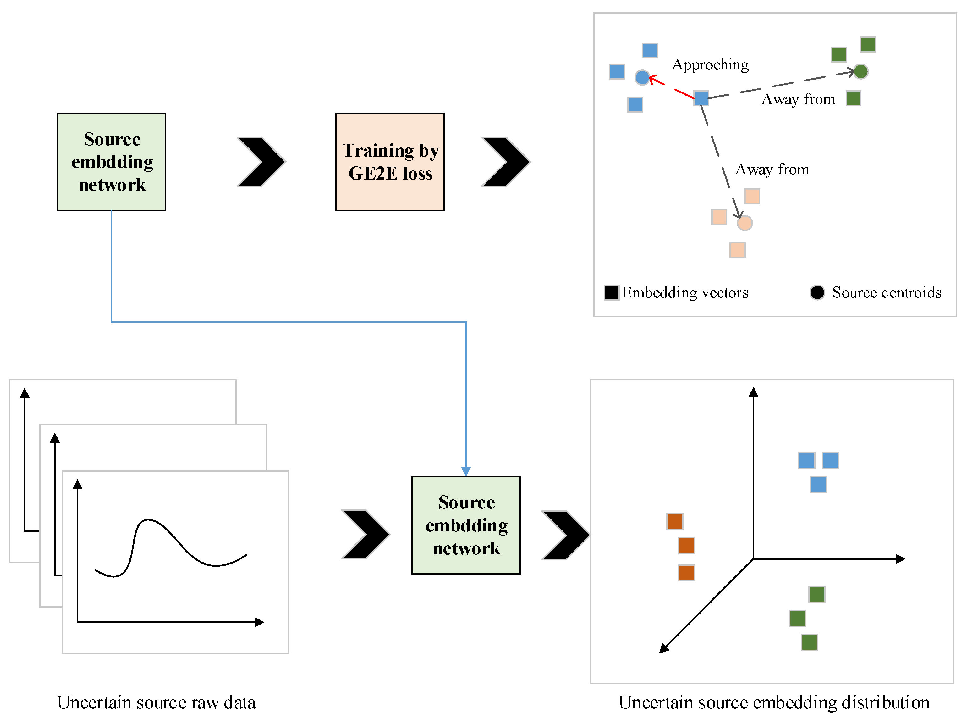
This study introduces the source embedding mechanism in the transformer. The source embedding mechanism is derived from the literature [30]. The literature [31] applied this mechanism to the power load clustering, and demonstrated that compared with traditional clustering methods, the source embedding mechanism can more effectively mine the statistical characteristics of uncertainty sources. This mechanism encodes any time series from a certain source into an embedding vector through a deep neural network. The embedding vectors of the same source are closer to their own centroid in high-dimensional space. These embedding vectors carry the statistical information of the source and can be used as input information by other neural networks for better prediction results.
In this study, the CBHG network [32] is used for encoding. For a training batch with K sources, each source has M training segments, the encoding calculation can be represented by Formula (5):
e k , m = C B H G x k , m C B H G x k , m 2
where e k , m is the encoding for the m-th time series segment x k , m of the k -th source. C B H G x k , m represents the output of the CBHG network after inputting x k , m . | | | | 2 represents taking the 2-norm. In this paper, the GE2E loss is used to train this encoding network, so that for any input segment x i of source i , an embedding vector e i can be output, which is closer to the centroid of source i in cosine distance and away from the centroids of other sources. The principle of GE2E loss is to construct a similarity matrix S for each training batch, whose elements are s p , m , where p 1 , , K × M . If p M = k ( represents rounding up), it means that these training data belong to source k and is the m -th training data. The calculation method of s p , m is shown in Formula (6):
s p , m = w c o s e k , m , c k p + b , p M = k w c o s e k , m , c k + b , o t h e r w i s e
where c k is the centroid of source k, whose calculation method is c k = 1 M m = 1 M e k , m . c k p is the centroid calculated when p M = k , excluding the current training data p, c k p = 1 M 1 m = 1 , m p % M M e k , m . c o s e k , m , c k represents cosine distance, c o s e k , m , c k = e k , m c k e k , m 2 c k 2 , w and b are the weight and bias parameters that need to be trained. It can be seen that when m = k , s p , m calculates the distance between the time series segment and its corresponding source k centroid. When m k , s p , m calculates the average distance between the time series segment and the centroids of all sources that do not belong to it. We hope that the former is smaller and the latter is larger. Therefore, the calculation method of the GE2E loss is shown in Formula (7):
L e p m = s p , m l o g s p , k
where p M = p M = k , p M k . Then, the total loss value of a training batch is calculated by Formula (8):
L O S S = L e p , m
If a database covering enough statistical patterns is used to train this encoding network, an embedding vector e is an output for any time series outside the training set. This vector carries good statistical properties and can provide effective information for the prediction network. The principle of the source embedding mechanism is shown in Figure 5.

3.3. Evaluation of Prediction Methods

This article uses the ENTSO-E database [24] to train the embedding network and transformer. The database is a data platform operated by the European Network of Transmission System Operators for Electricity (ENTSO-E), which aims to enhance the transparency and comparability of electricity market information in the European Union. The database includes spot price data for 20 markets and predicted wind power output data for ISO. This article collected local wind power data from 50 locations. The basic time interval of the data is 1 h. Based on these data, the node electricity price conditional prediction model p 1 x L M P y I S O w i n d N , θ 1 and local wind power conditional prediction model p 2 x l o c a l w i n d y I S O w i n d N , θ 2 were trained. Models p 1 and p 2 use the same hyperparameters and optimizer settings, as shown in Table 1.
This article randomly selected 10% of the data from the original dataset as the test set. Table 2 lists the evaluation results of the proposed method and traditional non-conditional probability-based LSTM [33], CNN [33], and sequence to sequence (seq2seq) [34] models on the test set. This article labeled node electricity price prediction as task1 and local wind power prediction as task2.

4. Bi-Level Optimization Model for Equilibrium Operation Strategy

4.1. Short-Term and Long-Term Operational Issues Faced by ADNO

Figure 1 shows the basic operating mode of ADNO, which is to buy electricity from the wholesale market and sell it to customers within the distribution network. We assume that the wholesale market is sufficiently competitive and that a single ADNO cannot affect the market price. Therefore, ADNO needs to make accurate predictions about the spot prices in the wholesale market. On the other hand, ADNO can influence customers’ demand by providing subsidies, as customers have different levels of price elasticity for electricity demand. Customers have some rigid demand that is almost unaffected by monetary incentives (such as essential electricity consumption for work and lighting), and some flexible demand that is influenced by possible subsidy amounts (such as demand for entertainment and comfort). Therefore, ADNO needs to predict the rigid demand and influence the flexible demand through subsidies. Since ADNO’s customers are limited and small-scale, they respond to ADNO’s subsidies individually, and it is difficult to define the collective response of customer groups to ADNO’s subsidy strategy using a specific statistical distribution method. In the short term, ADNO needs to optimize its internal power generation and energy storage scheduling based on the predicted spot market prices, local renewable energy output, and rigid loads. To find ADNO’s short-term equilibrium operation strategy, this paper proposes a bi-level optimization model based on the Stackelberg game. This model is constructed for ADNO in the day-ahead scheduling using the predicted spot market prices, wind power generation output, and load. Besides predicting renewable energy output and spot market prices accurately and setting subsidies appropriately, ADNO also faces the challenge of determining the optimal capacity of energy storage, internal renewable energy generation units, and fossil fuel generation units when investing in network assets. This is ADNO’s long-term operational strategy problem. Therefore, based on the short-term optimal solution, this paper introduces an efficiency measurement indicator. When this indicator reaches the marginal optimal value, it can determine ADNO’s optimal asset size in the long term.

4.2. Hedging Strategies of ADNO for Spot Wholesale Electricity Prices and Renewable Energy Output Fluctuations

4.2.1. Configuring Energy Storage Systems

Configuring energy storage systems is critical for ADNO. Energy storage systems allow ADNO to store electricity when spot wholesale prices are low or when there is excess renewable energy within the system, and release the stored electricity during opposite conditions to reduce costs. Assuming ADNO has S energy storage systems, and each system is numbered s , then s 1 , , S . Similarly, assuming a day is divided into T time slots, and each time slot is numbered t , then t 1 , , T . Let P s , t S T R C be the charging power of energy storage system s at time t , and P s , t S T R D be the discharging power of energy storage system s at time t . The following constraints apply, as shown in Equation (9):
0 P s , t S T R C 1 b s , t U s S T R C 0 P s , t S T R D b s , t U s S T R D t 1 , T , s 1 , , S
where U s S T R C is the maximum charging power of s , and U s S T R D is the maximum discharging power of s . b s , t is a binary variable that indicates whether s is charging (0) or discharging (1) at time t .
Furthermore, assuming the energy storage system s has a maximum capacity of U s E S T R , then the following constraints apply, as shown in Equation (10):
e s , t S T R = e s , t 1 S T R + P s , t S R T C P s , t S T R D Δ t 0 e s , t S T R U s E S T R t 1 , , T , s 1 , , S
where e s , t S T R represents the total stored electricity of s at time t , and Δ t represents the time interval.

4.2.2. Configuring Distributed Fossil Energy

Suppose ADNO has I fossil energy installed internally, and the label of each fossil energy unit is i , then i 1 , , I . A typical distributed fossil energy installation is a small gas turbine. The goal of installing internal power generation is to supplement the insufficient external power or to replace the expensive external power. Because these installations are relatively small, this article considers a simple linear cost model for fossil energy installation i as shown in Formula (11).
C o s t i = c i P i , t G E N + w i , t O i , t = 2 , , T
There are constraints on fossil energy unit i as shown in Formula (12):
L i G E N z i , t P i , t G E N U i G E N z i , t
where C o s t i represents the total production cost of i , c i is the marginal cost of i , P i , t G E N is the active power output of i at time t , and O i is the start-up cost of i . z i , t is a 0–1 variable. When it is 0, it means that i is in the shutdown state at time t ; when it is 1, it means that i is in the running state at time t . L i G E N is the minimum output of unit i , and U i G E N is the maximum output of unit i . There is:
w i , t = 1 , z i , t z i , t 1 = 1 , t = 2 , T 0 , o t h e r w i s e
The variable w i , t is also a 0–1 variable. When w i , t = 1 , i is started at time t , and its start-up cost needs to be calculated. Since i is a small unit, this article ignores its shutdown cost. There are multiple operating constraints for fossil energy installation i . In the active distribution network, the advantage of distributed fossil energy is that it can adjust its output quickly to cope with the fluctuations of renewable energy output and the spot price fluctuations of main grid electricity. Therefore, this article considers the ramp constraint as shown in Formula (14).
L i R A M P i , t G E N P i , t 1 G E N U i R A M , t = 2 , , T
where L i R A M is the minimum climbing amount of unit i between units, and U i R A M is the maximum climbing amount of unit i between units.

4.2.3. Configuring Distributed Wind Power Generation

ADNO has V distributed wind power generation units installed internally, each wind power generation unit is numbered v , and v is within 1 , , V . The advantage of ADNO’s distributed wind power generation installation is that wind power generation has almost zero marginal cost and can replace the electricity provided by the main grid at very low cost. However, distributed wind power generation also has strong randomness and uncontrollability. This article predicts the local wind power generation output through the method described in Section 3.

4.3. Customer Electricity Demand and Network Constraints

4.3.1. Customer Electricity Demand

This article assumes that ADNO’s customers have two types of loads: rigid loads (such as essential electricity consumption for work and lighting) and flexible loads (such as loads that can be shifted in time). Rigid loads are random and independent of other factors. Flexible loads depend on prices. Assuming ADNO has J customers, the electricity demand of customer j at time t is shown in Formula (15):
D e m a n d j , t = d j , t + d j , t ~ , j 1 , , J , t 1 , , T
where D e m a n d j , t is the total active power demand of customer j at time t , d j , t ~ is the rigid demand of customer j at time t , and d j , t is the flexible demand of customer j at time t . As the rigid demand of customers is not significantly correlated with the wind power output forecast of ISO, this article uses the method in reference [35] to predict their rigid demand.
This article assumes that the retail market is fully accurate and that ADNO cannot affect the retail electricity price p j , t . For flexible demand, ADNO can influence it through certain subsidy strategies, as follows:
d j , t D j , t s u b j , t , j 1 , , J , t 1 , , T
where D j , t is a set of demand responses to subsidies, and s u b j , t is ADNO’s subsidy strategy at time t . It can be seen that ADNO can influence the flexible demand of customers by subsidizing them when the spot price is low or when the wind is strong.
This article assumes that for all j 1 , , J , t 1 , , T , D j , t is a linear interval of d j , t , i.e.,:
L j , t d j , t U j , t , j 1 , , J , t 1 , , T
where L j , t = 0 . U j , t is influenced by p t , as shown in Formula (18):
U j , t = U j , t m a x + s u b j , t s u b m a x E l a j , t , j 1 , , J , t 1 , , T
where U j , t m a x is the maximum flexible demand of j at time t ; s u b j , t is the electricity subsidy that j can receive at time t ; s u b m a x is the maximum subsidy value. E l a j , t is the elasticity coefficient of the power demand subsidy for j at time t .

4.3.2. Network Constraints

The voltage level of the distribution network is relatively low, and the impact of transmission loss on ADNO operation needs to be considered. This paper constructs a network model constraint based on the standard distribution network branch model [36]. The power and voltage of nodes have linear constraints as shown in Formula (19):
P n = P m n I m n 2 r m n k n P n k Q n = Q m n I m n 2 x m n k n Q n k U n 2 = U m 2 2 r m n P m n + x m n Q m n + r m n 2 + x m n 2 I m n 2
where P n is the active power injected into node n , P m n is the active power flowing from node m to node n , Q n is the reactive power injected into node n , and Q m n is the reactive power flowing from node m to node n . I m n is the amplitude of the current flowing from node m to node n . r m n is the resistance of the line mn, and x m n is the reactance of the line mn. Expression k n means the set of nodes connected to node n on the network. U n is the voltage amplitude of node n . There are safety constraints for on-line voltage and circuit current:
I m n I m n m a x U n m i n U n U n m i n
At the same time, there is also a non-convex power balance constraint as shown in Formula (21):
I m n 2 u m = P m n 2 + Q m n 2
In this regard, this paper intends to perform second-order cone relaxation on this constraint to make it a convex constraint. As shown in Formula (22):
2 P m n 2 Q m n I m n 2 U m n 2 T 2 I m n 2 + U m n 2
The literature [37] shows that for distribution networks that meet certain conditions (such as IEEE33), after the above relaxation, the optimal solution of the new problem is also the optimal solution of the original problem. After second-order cone relaxation, the difficulty of solving the calculation is greatly reduced.

4.4. Stackelberg Game and Bi-Level Optimization Model

As mentioned in Section 4.1 and Section 4.3.1, there are two major assumptions.
Assumption 1.
The competition in the wholesale market is enough to be sufficient, and a single ADNO cannot affect the market price.
Assumption 2.
The retail market is fully accurate and ADNO cannot affect the retail electricity price.
Under these assumptions, a Stackelberg Game based bi-level optimization model can be established.
As mentioned in Section 4.1, the game between ADNO and customers can be modeled using the Stackelberg game. Based on the contents of Section 4.2 and Section 4.3, this text constructs a bi-level optimization model. In this article, we consider the following decision variables for ADNO in the current operating plan: P i , t G E N , P t R E A , P s , t S T R C , P s , t S T R D , w i , t , and b s , t . Here, q i , t G E N represents the active power dispatch of the i -th distributed fossil unit by ADNO at time t ; P t R E A represents the power purchase amount from the wholesale market by ADNO at time t ; P s , t S T R C represents the charging dispatch of the s -th distributed fossil unit by ADNO at time t ; P s , t S T R D represents the discharging dispatch of the s -th distributed fossil unit by ADNO at time t ; w i , t represents whether ADNO starts the i -th distributed fossil unit at time t , where 0 means not started and 1 means started; and b s , t represents whether the s -th energy storage device started at time t is in charging state (0) or discharging state (1).
For customers, they need to make demand decisions at a certain price level after ADNO makes operating decisions. According to Section 4.3.1, the demand variable for customers is d j , t , which represents the elastic electricity demand.
ADNO and customers have different decision objectives. ADNO aims to maximize revenue, while customers hope to minimize electricity costs. Therefore, a bi-level game model can be constructed for this Stackelberg game as shown in Formula (23). In Formula (23), the objective function of the upper-level problem is the maximization of the revenue of the ADNO. j = 1 J t = 1 T p t d j , t + d j , t ~ is the total electricity sale income. t = 1 T p t ^ P t R E A + i I c i P i , t G E N + O i w i , t + j = 1 J s u b j , t is the total cost, which contains the electricity import cost p t ^ P t R E A , fossil generation cost (consider start-up and shut-down cost) i I c i P i , t G E N + O i w i , t , and demand subsidy cost j = 1 J s u b j , t . The objective function of the upper-level problem is the minimization of the total cost of customers. As for the constraints, constraint (a) corresponds to the conditions stated in Section 4.2.1. Section 4.2.1 describes the constraints on operating variables P s , t S T R C and P s , t S T R D , and the variable set determined by these constraints is defined as Ω S T R . Therefore, P s , t S T R C , P s , t S T R D , and b s , t are elements of Ω S T R . Constraint (b) corresponds to the conditions stated in Section 4.2.2. Section 4.2.2 describes the constraints on the operating variable P i , t G E N , and the variable set determined by these constraints is defined as Ω G E N . Therefore, P i , t G E N and w i , t are elements of Ω G E N . Constraint (b) corresponds to the conditions stated in Section 4.3.2. Section 4.3.2 describes the network constraints, and the variable set determined by these constraints is defined as Ω N E T . Therefore, P i , t G E N , P t R E A , P s , t S T R C , P s , t S T R D , w i , t , and b s , t are elements of Ω N E T . Constraint (d) is the value positive constraint. Constraint (e) is the power balancing constraint. Constraint (e) corresponds to the subsidy constraint described by Formula (16). A bi-level game model can be constructed for this Stackelberg game as shown in Formula (23), and its detailed mathematical description is shown in Appendix A.
max q i , t GEN , P t REA , P s , t STRC , P s , t STRD , w i , t , b s , t , sub j , t j = 1 J t = 1 T p t d j , t + d j , t ~ t = 1 T p t ^ P t R E A + i I c i P i , t G E N + O i w i , t + j = 1 J s u b j , t s . t . P s , t S T R C , P s , t S T R D , b s , t Ω S T R P i , t G E N , w i , t Ω G E N P i , t G E N , P t R E A , P s , t S T R C , P s , t S T R D , w i , t , b s , t Ω N E T P t R E A 0 min d j , t j = 1 J t = 1 T p t d j , t + d j , t ~ s . t . j J d j , t + j J d j , t ~ + s S P t S T R C = P t R E A + i I P i , t G E N + s S P t S T R D + v V P v , t G E N d j , t D j , t s u b j , t
where p t ^ represents the spot price at time t ; P v , t G E N represents the output of the v -th wind power unit at time t ; d j , t represents the stochastic demand of the j -th customer at time t . They are predicted using the method described in Section 3 of this article.

4.5. Short-Term Equilibrium Solution and Long-Term Optimal Investment Analysis Method

It can be seen that the bi-level optimization model represented by Formula (23) has an upper layer model with a convex optimization model and a lower layer model with a linear optimization model. For such a model, the KKT conditions of the lower layer optimization can be added to the constraints of the upper layer optimization model, and the original bi-level optimization model can be transformed into a non-convex model with complementary relaxation equality constraints. The KKT transformed problem formulation is shown in Appendix A. This paper uses MOSEK (version 10) to find the global optimal solution to this problem.
The solution obtained based on this method is the short-term equilibrium solution for the active distribution network operation. In the long run, ADNO may achieve Pareto improvement through investment in energy storage, power generation, and other assets. In order to measure the degree of ADNO’s Pareto improvement, this paper proposes an indicator as shown in Formula (24).
E f f A D N O = E I n c o m e E C R E A + C G E N + C P U N
where E · represents the expectation. Income represents ADNO’s daily income; C R E A represents ADNO’s daily purchase cost from the wholesale market; C G E N represents ADNO’s daily generation cost; C P U N represents ADNO’s contract penalty cost caused by forecasting and scheduling deviations. Therefore, E f f A D N O can be expressed as shown in Formula (25):
E f f A D N O = E j = 1 J t = 1 T p t d j , t * + d j , t R l z ~ K E t = 1 T p t R l z ^ P t * , R E A + i I c i P i , t * , G E N + O i w i , t * + j = 1 J s u b j , t * + C p u n K
where the asterisk represents the equilibrium scheduling strategy in a period (day); R l z represents the realization value of uncertain quantities in a period (day); the subscript K represents the total number of experiments conducted. C p u n is the penalty value for ADNO based on the actual value of the unknown quantity. ADNO may be penalized in the following cases: ① The spot price estimate is too low, and local electricity could have been used instead; or the spot price estimate is too high, and too much more expensive local power generation is used. ② The output of local wind turbines is overestimated, and the insufficient part needs to be supplemented with more expensive power generation; the output of local wind turbines is underestimated, and more expensive local fossil energy or electricity spot is used. ③ The load forecast is underestimated, and more expensive electricity spot or local fossil energy needs to be supplemented; the load forecast is overestimated, and expensive electricity spot is purchased, which could have been replaced by local wind power generation.
To simplify, this paper calculates C p u n as C p u n = c C c r e a s o n , and the relationship is shown in Formula (26):
C c r e a s o n = p c r e a s o n q c r e a s o n
where C c r e a s o n represents one of the above three penalties, p c r e a s o n is the corresponding unit penalty cost, and q c r e a s o n is the corresponding deviation.

5. Case Study

5.1. IEEE 33 Test System and Main Experimental Parameters

This article tests the effectiveness of the proposed method on a modified IEEE 33 active distribution network. It is a modified version of the IEEE 33 bus radial distribution network [38], which is widely used in distribution system analysis [39,40,41]. Its baseline configuration is shown in Figure 6, with energy storage systems installed at nodes 1 and 5. Wind turbines are installed at nodes 4, 20, and 10, while small gas generators are installed at nodes 9, 23, and 26.
As described in Section 3, this paper trains the conditional prediction model and source embedding model based on 90% of the data in the dataset [24], and randomly extracts 10% of the data as test data for electricity wholesale prices and wind power output. We use the node load data in the dataset as the total real-time load sequence value of the IEEE 33 active distribution network, and obtain the baseline load capacity ratio of IEEE 33 nodes from literature [42]. We distribute the real-time load data according to the capacity ratio, and obtain the real-time load sequence of each load node. The real-time output data of wind power generation is also distributed in a similar way. The main hyperparameter models of the deep neural network model used in this paper are shown in Table 3.
The baseline data used in this article is shown in Table 4.

5.2. Ablation Experiment of The Forecast Model

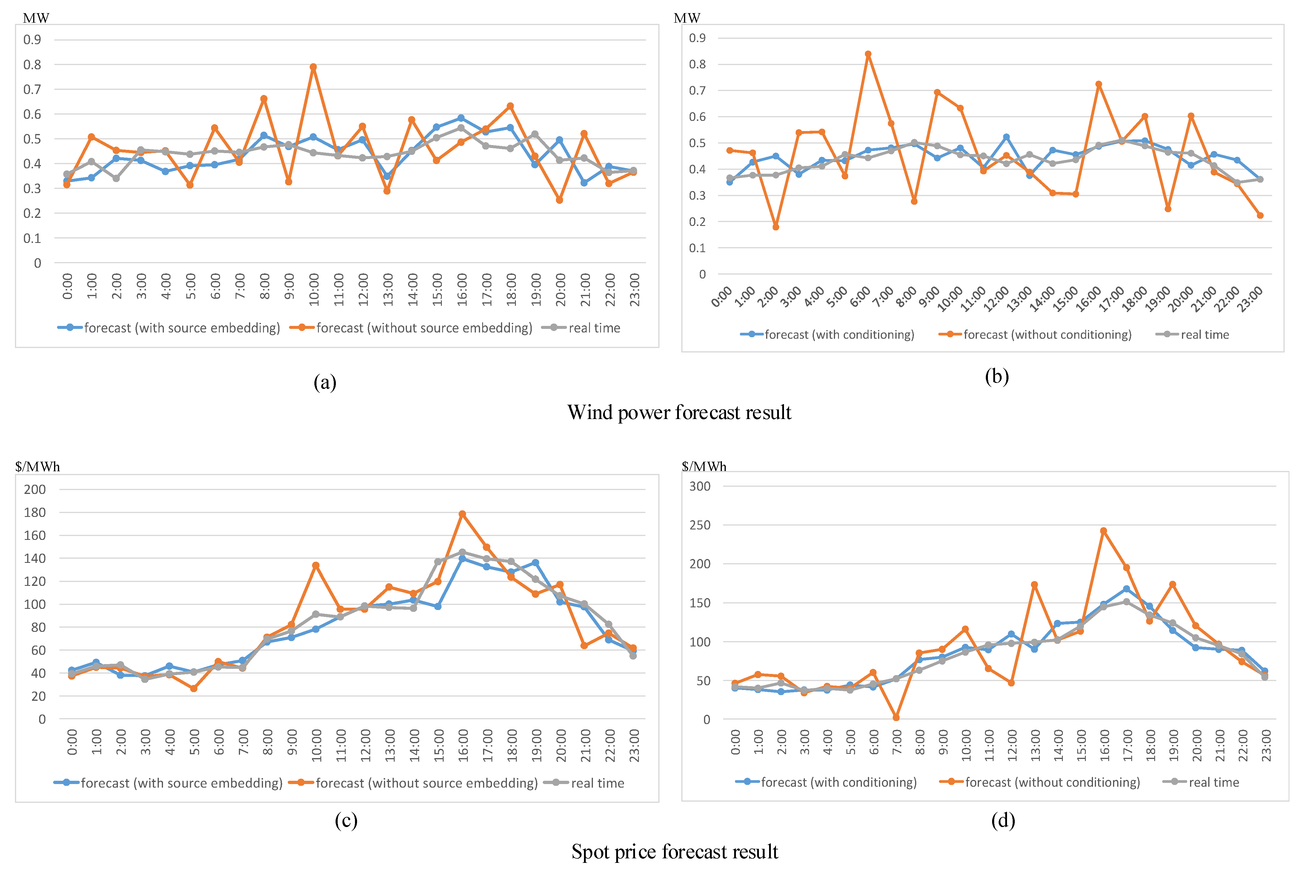
According to Section 3.1., in the case of high wind power penetration, there is a high correlation between wholesale electricity price, wind power output, and ISO predicted regional wind power output level. Therefore, in Section 3, this paper proposes a prediction method based on source embedding and conditional prediction. Based on the test data, the role of source embedding and conditional prediction proposed in this paper can be tested. For a typical day, this paper compares the role of source embedding and conditional forecasting in predicting short-term spot prices and local wind power output. The results are shown in Figure 7.
From Figure 7a,b, it can be seen that for local wind power prediction, source embedding can provide a certain improvement in prediction accuracy when conditional predictions are used. Moreover, this improvement is larger than the accuracy improvement from conditional prediction with source embedding. This may be because source embedding can effectively capture the statistical characteristics of wind power output in different geographical distributions, and the information it provides exceeds the role of conditional prediction.
From Figure 7c,d, we can see that for the spot price forecast, source embedding can provide a certain improvement in forecast accuracy when there are conditional forecasts. However, this improvement is smaller than the accuracy improvement from conditional prediction with source embedding. This may be because the spot price is greatly affected by random factors, and the statistical coding of big data can provide less effective information. However, under high wind power penetration, the system wind power has a significant impact on the spot price, which is easier to be captured by the conditional probability prediction model.
As a result, we can see that the source embedding method brings greater accuracy in wind power forecasting and the conditional method brings greater accuracy in price forecasting. When they are combined by our method, we obtain better results for both tasks.
This paper compares the control variables of these two factors in the test set and shows the results in Table 5. We denote the node electricity price prediction as task1 and the local wind power prediction as task2.

5.3. Equilibrium Scheduling and Short-Term Optimal Strategy

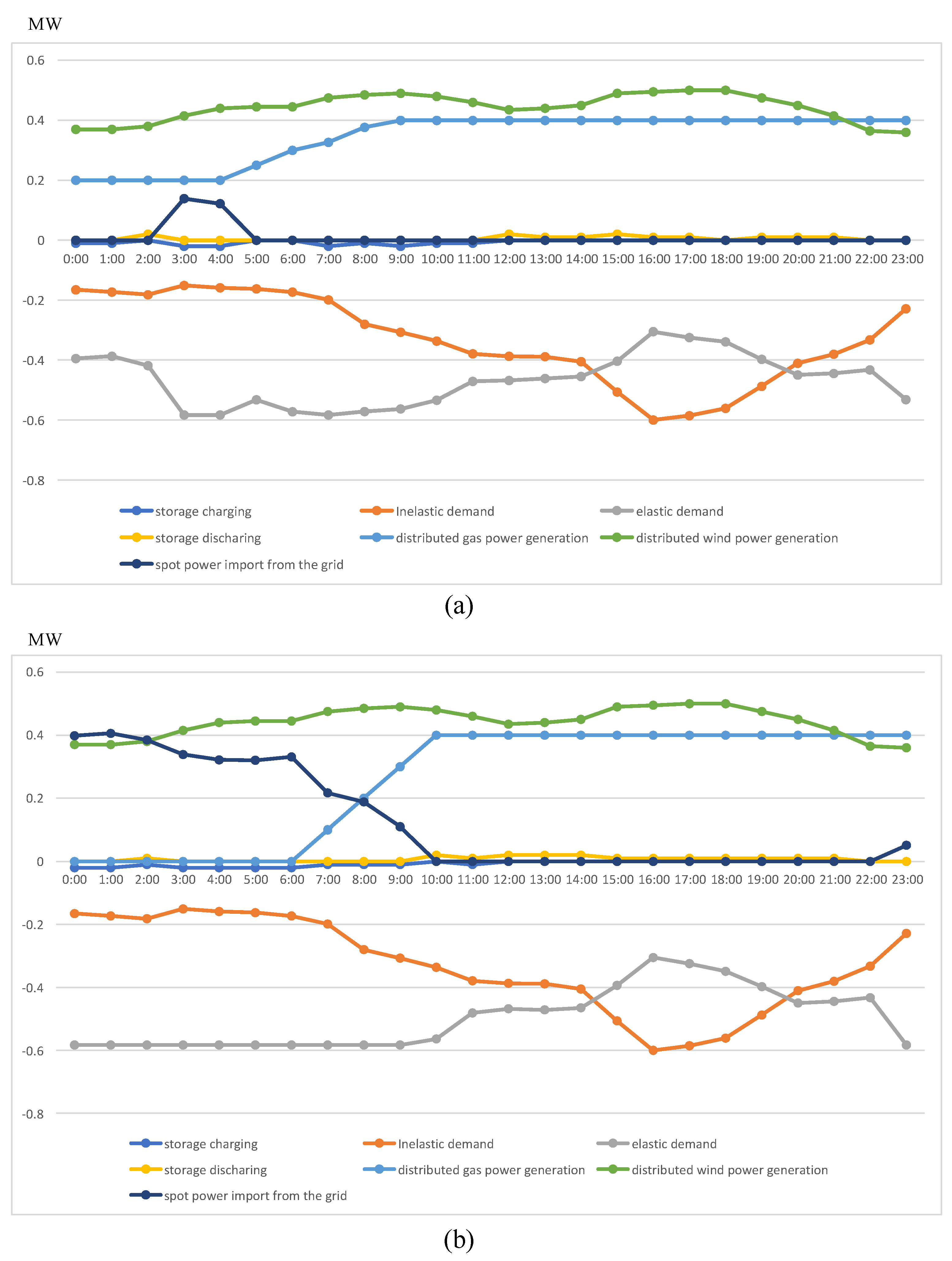
Figure 8 shows the effectiveness of the short-term equilibrium scheduling method proposed in this study. The baseline system in this paper has high wind power penetration. During the time period from 0:00 to 9:00 when the spot price is relatively low, through the method proposed in this paper, ADNO can motivate customers to increase elastic demand. At this time, a large number of elastic loads are excited to make use of cheap wind energy. Since the spot price is higher than the marginal cost of internal distributed gas-fired power generation, ADNO relies on local wind power and gas-fired power generation to meet the load demand during the peak period of electricity consumption from 9:00 to 18:00. From 0:00 to 3:00 when the spot price is the cheapest, ADNO purchases a part of the electricity spot and stores it based on energy storage equipment, and releases it during the peak period of electricity consumption from 9:00 to 18:00 to meet the load demand, as shown in Figure 8a.
If the spot price changes, ADNO’s equilibrium scheduling result changes significantly. The dispatch result shown in Figure 8b is the case where the average spot price is reduced to 50% of the original. At this time, the spot price from 0:00 to 9:00 is cheap enough. During this time period, ADNO reduced local gas-fired power generation, fully imported a large amount of spot goods, and increased incentives for customers to flexibly load. It can be seen that based on the method proposed in this paper, ADNO can effectively respond to the spot price of the main network. If the main grid wind power output is too large, resulting in a drop in spot prices, ADNO can increase the consumption of main grid wind power by dispatching energy storage and stimulating loads. If the main grid power generation capacity is insufficient and the spot price rises, ADNO can dispatch local wind power and gas generators to meet the power demand, or reduce the elastic demand of customers through incentives. In this process, clean energy has always been provided priority. The potential for this level of response is far greater than that of a single load, or of an unorganized distribution network.
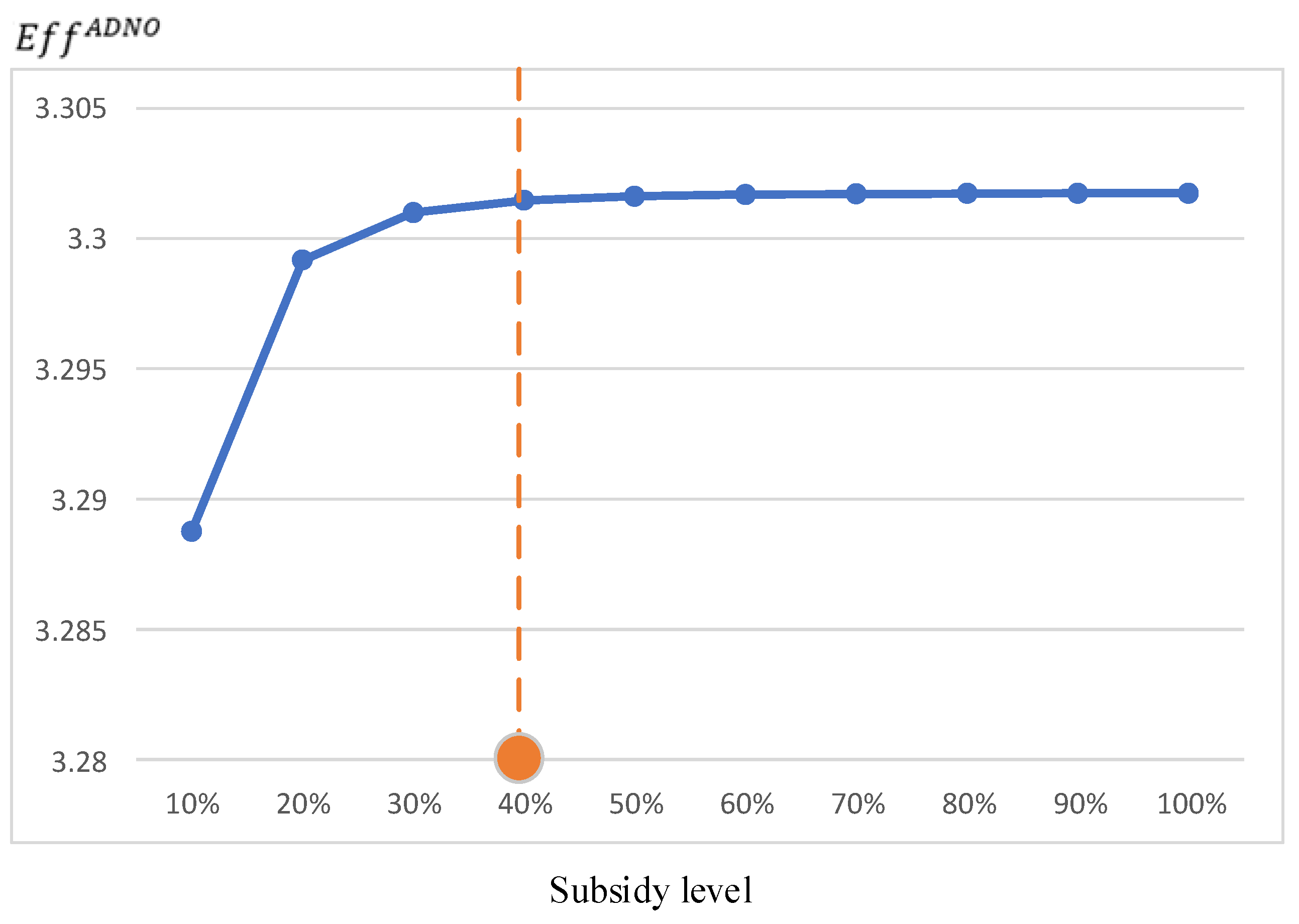
From a short-term subsidy strategy point of view, ADNO also has an optimal subsidy level. It can be seen that there is an optimal value of ADNO’s subsidy incentives for customers, as shown in Figure 9. The vertical axis is the ADNO efficiency index shown in Formula (24), and the horizontal axis is the level of subsidies relative to the benchmark value. Below this value, efficiency of ADNO can be improved through subsidies. However, beyond this value, increasing subsidies cannot further improve the efficiency of ADNO.
By controlling the variables, the effectiveness of the prediction method proposed in the third section and the game equilibrium scheduling method proposed in the fourth section can be demonstrated, and the results are shown in Table 6. It can be seen from the table that since the prediction method proposed in this paper can achieve lower average prediction errors, the penalty value can be reduced, thereby improving the E f f A D N O index value. The two-tier optimization model proposed in this paper considers the adjustment effect of ADNO subsidies on user demand. The results show that in the equilibrium outcome, there is room for the benefit brought by the subsidy to exceed the cost of the subsidy. Compared with the single-level optimization model, the method proposed in this paper can further improve the operating efficiency of ADNO.

5.4. Sensitivity to Long-Term Factors

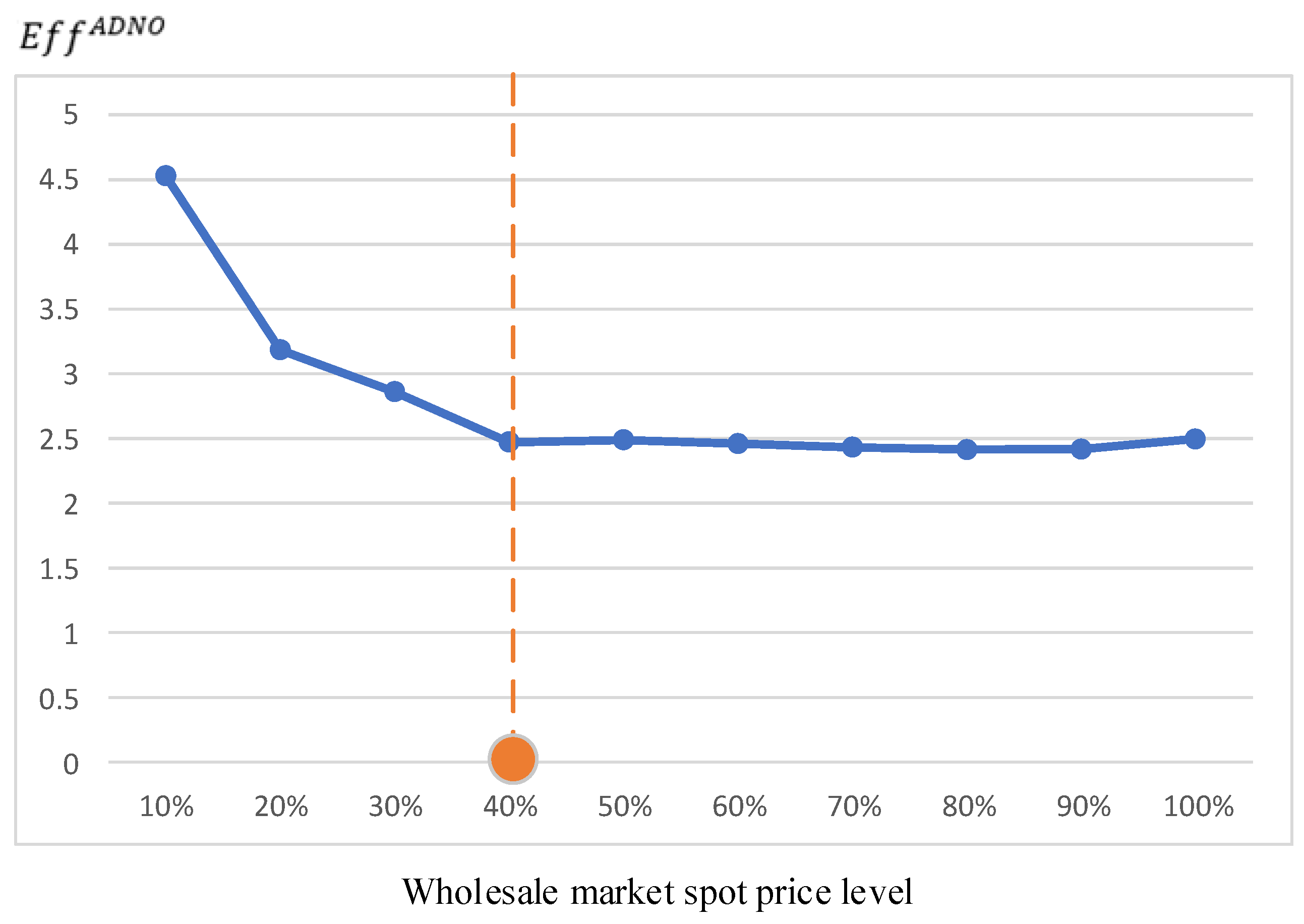
Firstly, this article examines the impact of long-term average spot electricity price levels on the profitability indicator E f f A D N O of ADNO. When the long-term average spot electricity price levels fluctuate between 10% and 100% of the benchmark values shown in Table 4, the change trend of E f f A D N O is shown in Figure 10. It can be seen from the graph that the spot price has about a 50% fluctuation range on the profitability of ADNO, indicating that spot prices have a significant impact on ADNO’s return on investment. It is worth noting that the impact of spot price levels on E f f A D N O is marginally decreasing. In this example, when the spot price exceeds 40% of the benchmark value, it has almost no impact on E f f A D N O . This is because within this range, ADNO can adjust its demand, comprehensively dispatch gas and wind power generators, and reduce power imports from the main grid to maintain the profitability at a certain level.
This reflects that the method proposed in this article can provide a “safeguard boundary” for ADNO against the fluctuation of spot prices in the main grid. When the fluctuation of spot prices exceeds this “safeguard boundary”, the profitability of ADNO can be guaranteed. This shows the robustness of our method to price variation.
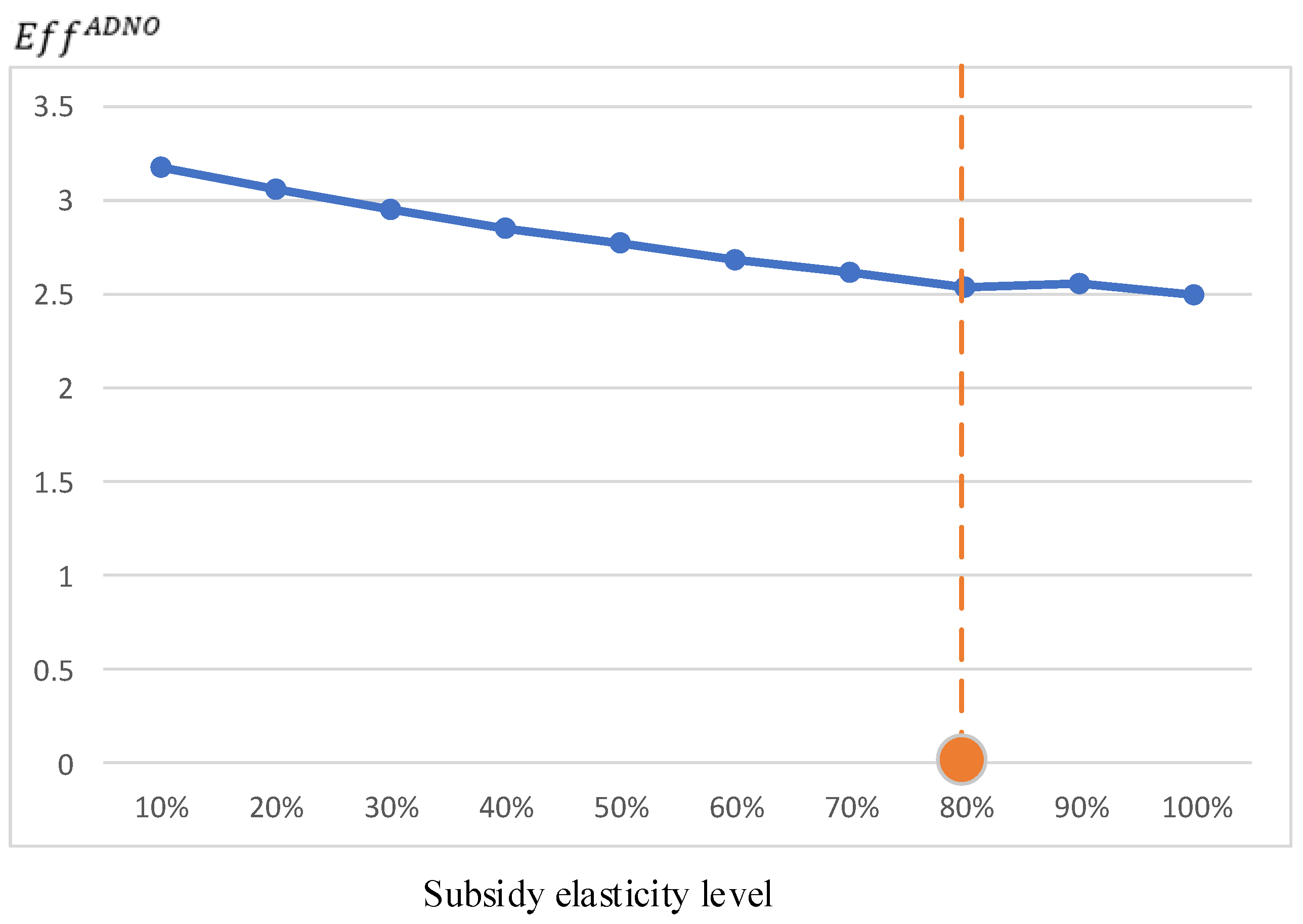
Secondly, this article examines the impact of the elasticity coefficient E l a j , t of subsidies on the yield indicator E f f A D N O of ADNO. When the mean elasticity coefficient of long-term average subsidies fluctuates between 10% and 100% of the benchmark value shown in Table 4, the trend of E f f A D N O change is shown in Figure 11. It can be seen from the figure that the impact of the elasticity coefficient of subsidies on the yield indicator is about 20%. For ADNO, the smaller the elasticity coefficient of demand for subsidies, the higher the yield rate of ADNO. Compared with the spot price, there is also a turning point in the impact effect of the elasticity coefficient, which is about 80% of the benchmark value. After the elasticity coefficient exceeds 80% of the benchmark value, it almost has no impact on E f f A D N O . This is because after the elasticity coefficient exceeds this turning point, due to the high cost of subsidies, ADNO almost no longer stimulates users’ elastic demand.
This means that as long as the elasticity coefficient of demand for subsidies is within a reasonable range, ADNO can improve its own revenue by subsidizing users. This shows the robustness of our method to the subsidy elasticity level.
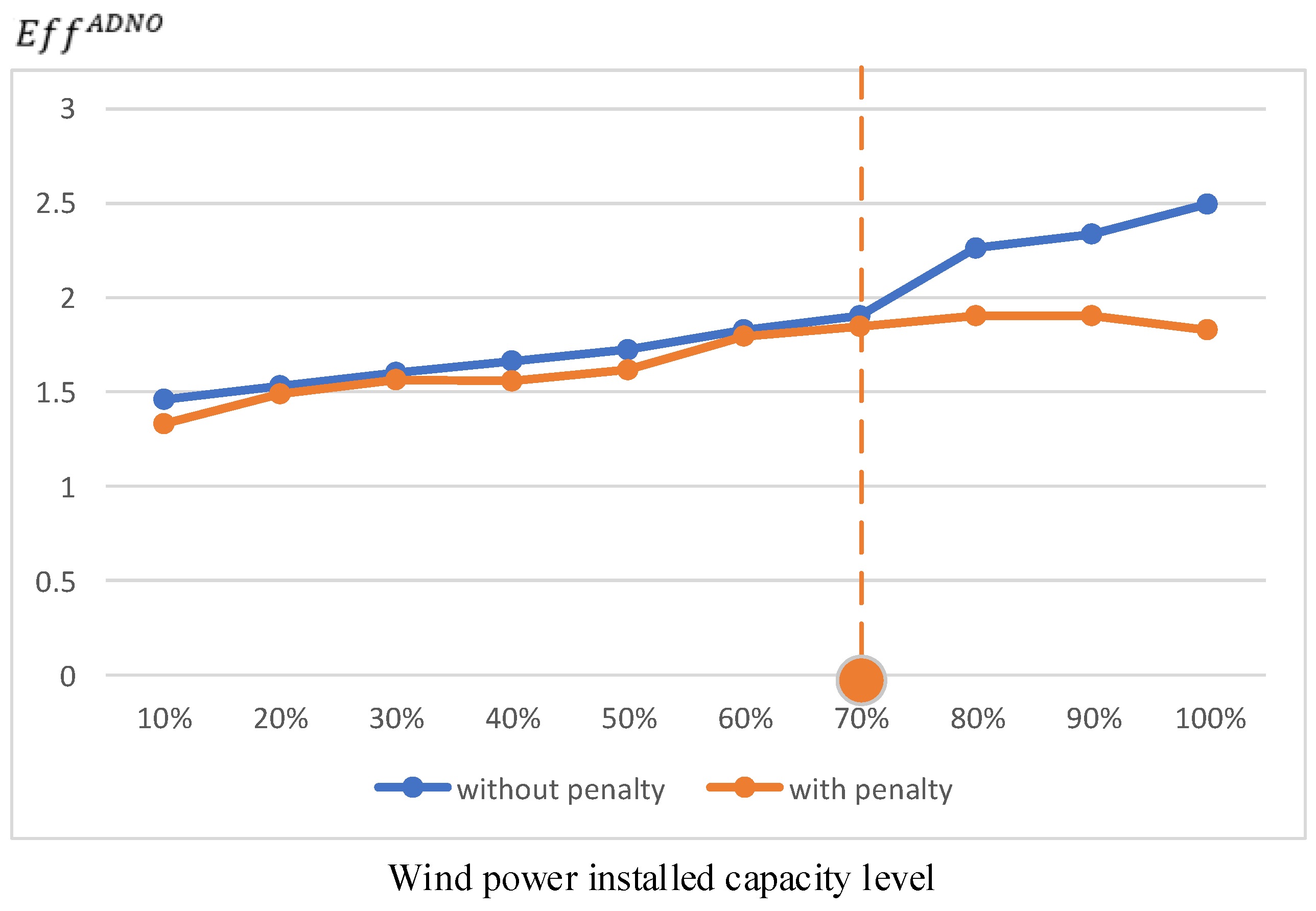
This article also examines the impact of wind power installed capacity on the profitability indicator E f f A D N O . When the wind power installed capacity fluctuates between 10% and 100% of the benchmark value shown in Table 4, the change trend of E f f A D N O is shown in Figure 12. If the penalty cost is not taken into account, the increase in wind power installed capacity can always bring positive returns to ADNO. However, if the uncertainty caused by the increase in wind power installed capacity leads to prediction errors and economic penalties, there is also a turning point in the impact of wind power installed capacity on the return on investment of ADNO, as shown in Figure 12.
When the wind power installed capacity exceeds this turning point, the return on investment of ADNO will show a slow downward trend. This shows the robustness of our method to wind power installed capacity.

6. Conclusions

As the penetration rate of variable renewable energy such as wind power increases gradually in the power system, the composition and balance of the power system also changes gradually. The intermittency of renewable energy challenges the stability of the traditional centralized generation and load-based transmission and distribution methods at high proportions of renewable energy penetration. Therefore, the Active Distribution Network Operator (ADNO) with distributed installation at the local level has a good application prospect in the new scenario. However, ADNO faces the issue of how to improve operational efficiency based on the types of local power generation and energy storage installations and the nature of the market environment. In this regard, this paper proposes a forecasting method that considers the coupling fluctuations of spot electricity prices and renewable energy, as well as a bi-level optimization operation method based on Stackelberg game for operation optimization of small-scale ADNO under high wind power penetration rate. There are three major findings.
  • The proposed conditional prediction method is effective. By analyzing the spot electricity price and wind power output data under high wind power penetration rate, this paper indicates the significant correlation between the two with zero time lag; therefore, this paper proposes a method based on ISO wind power prediction, which predicts the local wind power output and spot wholesale electricity price conditions. The method combines conditional prediction, transformer deep neural network, and a source embedding method, and improves the prediction accuracy compared with traditional prediction methods. The improvement in prediction accuracy helps to reduce the penalty cost in ADNO operation and improve operational efficiency.
  • A subsidy strategy may further improve the profitability of an ADNO. This paper proposes a subsidy strategy that considers the impact of ADNO on user demand. Under this subsidy strategy, a Stackelberg game is formed between the ADNO and users. This paper proposes a game model and its solution method that considers the spot electricity price of the main grid, local wind power output, local gas power generation, local energy storage, and network constraints simultaneously. Through simulation calculations, it is found that the comprehensive predictive method and bi-level optimization method proposed in this paper can indeed further improve the operational efficiency of ADNO compared with traditional methods.
  • The proposed model is robust to external long-term factors. This paper compares the impact of long-term factors under the methods proposed in this paper. It is found that the methods proposed in this paper can provide a “guarantee boundary” for the fluctuation of factors such as the spot price of the main grid and the elasticity of user subsidies. When the fluctuation of factors exceeds this “guarantee boundary”, the profitability of ADNO can be guaranteed.
However, there are some aspects that need to be attended to in future studies. Firstly, the improvement is limited to the scenario where local wind power fluctuation is correlated to grid-level wind power fluctuation, otherwise the conditionality may be missing. Secondly, the computation may be time consuming as the optimization model is non-convex, especially for large-scale problems. Although this paper focuses on the off-line application, further attention may be needed for on-line applications.

Author Contributions

Conceptualization, Y.S. and R.X.; methodology, F.L.; software, F.L.; investigation, M.J.; writing—original draft, Y.S. and H.L.; writing—review and editing, M.J. and X.G.; visualization, H.L.; supervision, Y.S. All authors have read and agreed to the published version of the manuscript.

Funding

This research was funded by State Grid Jilin Electric Power Co., Ltd. 2022 science and technology “Jie Bang Gua Shuai” project, grant number 2022JBGS-05.

Data Availability Statement

Not applicable.

Conflicts of Interest

The authors declare no conflict of interest.

Nomenclatures

P s , t S T R C ,   P s , t S T R D Charging and discharging power of energy storage system s at time t
U s S T R C , U s S T R D Maximum charging/discharging power of s
b s , t Binary value indicate charging or discharging
e s , t S T R Total stored electricity of s at time t
Δ t Time interval
P i , t G E N Active power output of i at time t
C o s t i Total production cost of i
O i start-up cost of i
L i G E N , U i G E N Minimum and Maximum output of unit i
L i R A M ,   U i R A M Minimum and Maximum climbing amount of unit i between units
p j , t Retail electricity price of customer j at time t
D e m a n d j , t Total active power demand of customer j at time t
d j , t , d j , t ~ Rigid and flexible demand of customer j at time t
D j , t Set of demand responses to subsidies
s u b j , t ADNO’s subsidy strategy at time t
E l a j , t Elasticity coefficient of the power demand subsidy for j at time t.
P n , Q n Active and reactive power injected into node n
P m n , Q m n Active and reactive power flowing from node m to node n
I m n Amplitude of the current flowing from node m to node n
U n Voltage amplitude of node n
Ω The variable set determined by constraints
p t ^ Spot price at time t;
E f f A D N O ADNO’s profitability indicator
KTotal number of experiments conducted
C G E N ADNO’s daily generation cost
C P U N ADNO’s contract penalty cost caused by forecasting and scheduling deviations
P t R E A Power purchase amount from the wholesale market by ADNO at time t

Appendix A

Formula (22) is a simplified form of the bi-level model. A detailed mathematical description of the bi-level is shown in Formula (A1).
m a x q i , t G E N , q t R E A , q s , t S T E C , q s , t S T R D , ϕ i , t G E N , ϕ v , t G E N , ϕ i , t S T R C , ϕ i , t S T R D , w i , t , b s , t F = j = 1 J t = 1 T p t d ¯ j , t + d ~ j , t t = 1 T p ^ t q t R E A + i I c i q i , t G E N + O i w i , t + j = 1 J s u b j , t s . t . L i R A M q i , t G E N q i , t 1 G E N U i R A M t = 2 , , T 0 q s , t S T E C 1 b s , t U s S T R C 0 q s , t S T E D b s , t U s S T R D e s , t S T R = e s , t 1 S T R + q s , t S R T C q s , t S T R D Δ t 0 e s , t S T R U s E S T R q t R E A 0 U n 2 = U m 2 2 r m n P m n + x m n Q m n + r m n 2 + x m n 2 I m n 2 I m n I m n m a x U n m i n U n U n m i n 2 P m n 2 Q m n I m n 2 U m n 2 T 2 I m n 2 + U m n 2 L t G E N z i , t q i , t G E N U t G E N z i , t w i , t = 1 ,   z i , t z i , t 1 = 1 0 ,   o t h e r w i s e min d ¯ j , t ϕ ¯ j , t j = 1 J t = 1 T p t d ¯ j , t + d j , t ~ s . t . P n , t G n q t R E A + j n q i , t G E N + s n q i , t S T R D + v n q v , t G E N s n q i , t S T R C j n d ¯ j , t j n d ~ j , t L 1 P n , t G n q t R E A + j n q i , t G E N + s n q i , t S T R D + v n q v , t G E N s n q i , t S T R C j n d ¯ j , t j n d ~ j , t L 2 Q n , t G n ϕ t R E A + j n ϕ i , t G E N + v n ϕ v , t G E N j n ϕ ¯ j , t j n ϕ ~ j , t L 3 Q n , t G n ϕ t R E A + j n ϕ i , t G E N + v n ϕ v , t G E N j n ϕ ¯ j , t j n ϕ ~ j , t L 4 L j , t A C T s u b j , t d ¯ j , t U j , t A C T s u b j , t L 5 L j , t R E A s u b j , t ϕ ¯ j , t U j , t R E A s u b j , t L 6
In Formula (A1), G n is a 0–1 parameter indication whether node n is the interface node that connects the distribution network and the grid. Variable ϕ t R E A is the reactive power imported by ADNO in time t. Variable ϕ i , t G E N is the reactive power generated by fossil unit i in time t. Parameter ϕ v , t G E N is the reactive power generated by VRE unit i in time t. Variable ϕ j , t is the lower level decision variable of reactive power consumption. Variable ϕ j , t is the lower level decision variable of reactive power consumption by customer j in time t. Parameter ϕ j , t ~ is the uncontrolable reactive power consumption by customer j in time t.
The lower level problem is a relatively simple linear problem. This makes the whole problem relatively more solvable. We substitute the lower level problem with its KKT condition. The KKT transformed problem formulation is shown in Formula (A2).
m a x q i , t G E N , q t R E A , q s , t S T E C , q s , t S T R D , ϕ i , t G E N , ϕ v , t G E N , ϕ i , t S T R C , ϕ i , t S T R D , w i , t , b s , t F = j = 1 J t = 1 T p t d ¯ j , t + d ~ j , t t = 1 T p ^ t q t R E A + i I c i q i , t G E N + O i w i , t + j = 1 J s u b j , t s . t . Original Upper level conditions o n d i t o n L 1 , L 2 , L 3 , L 4 , L 5 , L 6 p t d i a g λ T × A x b μ T x 0 λ T A x b = 0 μ T x = 0 λ 0 μ 0
In Formula (A2), x is the original lower level decision variable vector d 1,1 , d 1 , T , d 2,1 , d 2 , T , d J , 1 , d J , T , ϕ 1,1 , ϕ 1 , T , ϕ 2,1 , ϕ 2 . T , ϕ J , 1 , ϕ J , T T ·   d i a g is a J T × J T diagnal matrix with all diagnal entries equal to 1. A is a parameter matrix decided by condition (L1, L2, L3, L4, L5, and L6), which is not shown here due to its huge length. However, since the original lower problem is pure linear, matrix A is basiclly very simple to achieve. A is a 4 + 8 J T × 2 J T shaped matrix. b is a a 4 + 8 J T shaped matrix. λ and μ are the Lagrangian coefficients. λ is a 4 + 8 J T × 1 shaped vector. μ is a 1 × 2 J T shaped vector.

References

  1. Zhao, J.; Wang, C.; Zhao, B.; Lin, F.; Zhou, Q.; Wang, Y. A Review of Active Management for Distribution Networks: Current Status and Future Development Trends. Electr. Mach. Power Syst. 2014, 42, 280–293. [Google Scholar] [CrossRef]
  2. Xiang, Y.; Han, W.; Zhang, J.; Liu, J.; Liu, Y. Optimal Sizing of Energy Storage System in Active Distribution Networks Using Fourier-Legendre Series based State of Energy Function. IEEE Trans. Power Syst. 2017, 33, 2313–2315. [Google Scholar] [CrossRef]
  3. Ge, S.; Wang, S.; Lu, Z.; Liu, H. Substation planning method in an active distribution network under low-carbon economy. J. Mod. Power Syst. Clean Energy 2015, 3, 468–474. [Google Scholar] [CrossRef] [Green Version]
  4. Li, Z.; Wang, H.; Ai, Q.; Zhang, Y. Interactive optimization between active distribution network with multi-microgrids based on distributed algorithm. Energy Rep. 2020, 6, 385–391. [Google Scholar] [CrossRef]
  5. Xiao, J.; Qibo, H.E.; Guoqiang, Z.U. Distribution management system framework based on security region for future low carbon distribution systems. J. Mod. Power Syst. Clean Energy 2015, 3, 12. [Google Scholar] [CrossRef] [Green Version]
  6. Usman, M.; Coppo, M.; Bignucolo, F.; Turri, R. Losses management strategies in active distribution networks: A review. Electr. Power Syst. Res. 2018, 163, 116–132. [Google Scholar] [CrossRef]
  7. Gabash, A.; Li, P. Active-Reactive Optimal Power Flow in Distribution Networks with Embedded Generation and Battery Storage. IEEE Trans. Power Syst. 2012, 27, 2026–2035. [Google Scholar] [CrossRef]
  8. Cortes, C.A.; Contreras, S.F.; Shahidehpour, M. Microgrid Topology Planning for Enhancing the Reliability of Active Distribution Networks. IEEE Trans. Smart Grid 2017, 9, 6369–6377. [Google Scholar] [CrossRef]
  9. Kyriakou, D.G.; Kanellos, F.D. Optimal Operation of Microgrids Comprising Large Building Prosumers and Plug-in Electric Vehicles Integrated into Active Distribution Networks. Energies 2022, 15, 6182. [Google Scholar] [CrossRef]
  10. Sedghi, M.; Ahmadian, A.; Pashajavid, E.; Aliakbar-Golkar, M. Storage scheduling for optimal energy management in active distribution network considering load, wind, and plug-in electric vehicles uncertainties. J. Renew. Sustain. Energy 2015, 7, 033120. [Google Scholar] [CrossRef]
  11. Jiang, T.; Li, Z.; Jin, X.; Chen, H.; Li, X.; Mu, Y. Flexible operation of active distribution network using integrated smart buildings with heating, ventilation and air-conditioning systems. Appl. Energy 2018, 226, 181–196. [Google Scholar] [CrossRef]
  12. Chen, F.; Dong, L.; Xiong, X. Research on Stochastic Optimal Operation Strategy of Active Distribution Network Considering Intermittent Energy. Energies 2017, 10, 522. [Google Scholar] [CrossRef] [Green Version]
  13. Wang, J.; Zheng, X.; Tai, N.; Wei, W.; Li, L. Resilience-Oriented Optimal Operation Strategy of Active Distribution Network. Energies 2019, 12, 3380. [Google Scholar] [CrossRef] [Green Version]
  14. Tostado-Véliz, M.; Hasanien, H.M.; Jordehi, A.R.; Turky, R.A.; Gómez-González, M.; Jurado, F. An Interval-based privacy–Aware optimization framework for electricity price setting in isolated microgrid clusters. Appl. Energy 2023, 340, 121041. [Google Scholar] [CrossRef]
  15. Fan, S.; He, G.; Zhou, X.; Cui, M. Online optimization for networked distributed energy resources with time-coupling constraints. IEEE Trans. Smart Grid 2020, 12, 251–267. [Google Scholar] [CrossRef]
  16. Saint-Pierre, T.; Mancarella, P. Scheduling model for active distribution system management with renewable energy sources. IETGener. Transm. Distrib. 2017, 11, 1571–1579. [Google Scholar]
  17. Shen, X.; Shahidehpour, M.; Han, Y.; Zhu, S.; Zheng, J. Expansion planning of active distribution networks with centralized and distributed energy storage systems. IEEE Trans. Sustain. Energy 2016, 8, 126–134. [Google Scholar] [CrossRef]
  18. Yu, Q.; Li, Z. Correlated load forecasting in active distribution networks using Spatial-Temporal Synchronous Graph Convolutional Networks. IET Energy Syst. Integr. 2021, 3, 355–366. [Google Scholar] [CrossRef]
  19. Kalantar-Neyestanaki, M.; Sossan, F.; Bozorg, M.; Cherkaoui, R. Characterizing the reserve provision capability area of active distribution networks: A linear robust optimization method. IEEE Trans. Smart Grid 2019, 11, 2464–2475. [Google Scholar] [CrossRef]
  20. Cheng, G.; Song, S.; Lin, Y.; Huang, Q.; Lin, X.; Wang, F. Enhanced state estimation and bad data identification in active power distribution networks using photovoltaic power forecasting. Electr. Power Syst. Res. 2019, 177, 105974. [Google Scholar] [CrossRef]
  21. Cong, P.; Tang, W.; Zhang, L.; Zhang, B.; Cai, Y. Day-ahead active power scheduling in active distribution network considering renewable energy generation forecast errors. Energies 2017, 10, 1291. [Google Scholar] [CrossRef] [Green Version]
  22. Gao, H.; Liu, J.; Wang, L. Robust coordinated optimization of active and reactive power in active distribution systems. IEEE Trans. Smart Grid 2017, 9, 4436–4447. [Google Scholar] [CrossRef]
  23. Saint-Pierre, A.; Mancarella, P. Active Distribution System Management: A Dual-Horizon Scheduling Framework for DSO/TSO Interface Under Uncertainty. IEEE Trans. Smart Grid 2017, 8, 2186–2197. [Google Scholar] [CrossRef]
  24. ENTSO-E Transparency Platform. Available online: https://www.entsoe.eu/data/ (accessed on 23 April 2023).
  25. Hassan, M.A.; Bailek, N.; Bouchouicha, K.; Nwokolo, S.C. Ultra-short-term exogenous forecasting of photovoltaic power production using genetically optimized non-linear auto-regressive recurrent neural networks. Renew. Energy 2021, 171, 191–209. [Google Scholar] [CrossRef]
  26. Li, G.; Wang, H.; Zhang, S.; Xin, J.; Liu, H. Recurrent neural networks based photovoltaic power forecasting approach. Energies 2019, 12, 2538. [Google Scholar] [CrossRef] [Green Version]
  27. Alipour, M.; Aghaei, J.; Norouzi, M.; Niknam, T.; Hashemi, S.; Lehtonen, M. A novel electrical net-load forecasting model based on deep neural networks and wavelet transform integration. Energy 2020, 205, 118106. [Google Scholar] [CrossRef]
  28. Wang, H.; Lei, Z.; Zhang, X.; Zhou, B.; Peng, J. A review of deep learning for renewable energy forecasting. Energy Convers. Manag. 2019, 198, 111799. [Google Scholar] [CrossRef]
  29. Vaswani, A.; Shazeer, N.; Parmar, N.; Uszkoreit, J.; Jones, L.; Gomez, A.N.; Kaiser, Ł.; Polosukhin, I. Attention is all you need. Adv. Neural Inf. Process. Syst. 2017, 30, I. [Google Scholar]
  30. Wan, L.; Wang, Q.; Papir, A.; Moreno, I.L. Generalized end-to-end loss for speaker verification. In Proceedings of the 2018 IEEE International Conference on Acoustics, Speech and Signal Processing (ICASSP), IEEE, Calgary, AB, Canada, 15–20 April 2018; pp. 4879–4883. [Google Scholar]
  31. Ruhang, X. Efficient clustering for aggregate loads: An unsupervised pretraining based method. Energy 2020, 210, 118617. [Google Scholar] [CrossRef]
  32. Wang, Y.; Skerry-Ryan, R.J.; Stanton, D.; Wu, Y.; Weiss, R.J.; Jaitly, N.; Yang, Z.; Xiao, Y.; Chen, Z.; Bengio, S.; et al. Tacotron: Towards end-to-end speech synthesis. arXiv 2017, arXiv:1703.10135, 2017. [Google Scholar]
  33. Ugurlu, U.; Oksuz, I.; Tas, O. Electricity price forecasting using recurrent neural networks. Energies 2018, 11, 1255. [Google Scholar] [CrossRef] [Green Version]
  34. Wang, Y.; Zou, R.; Liu, F.; Zhang, L.; Liu, Q. A review of wind speed and wind power forecasting with deep neural networks. Appl. Energy 2021, 304, 117766. [Google Scholar] [CrossRef]
  35. Zhao, Q.; Shen, Y.; Li, M. Control and bidding strategy for virtual power plants with renewable generation and inelastic demand in electricity markets. IEEE Trans. Sustain. Energy 2015, 7, 562–575. [Google Scholar] [CrossRef]
  36. Antoniadou-Plytaria, K.E.; Kouveliotis-Lysikatos, I.N.; Georgilakis, P.S.; Hatziargyriou, N.D. Distributed and Decentralized Voltage Control of Smart Distribution Networks: Models, Methods, and Future Research. IEEE Trans. Smart Grid 2017, 8, 2999–3008. [Google Scholar] [CrossRef]
  37. Li, Y.; Xiao, J.; Chen, C.; Tan, Y.; Cao, Y. Service restoration model with mixed-integer second-order cone programming for distribution network with distributed generations. IEEE Trans. Smart Grid 2018, 10, 4138–4150. [Google Scholar] [CrossRef]
  38. Baran, M.E.; Wu, F.F. Network reconfiguration in distribution systems for loss reduction and load balancing. IEEE Trans. Power Deliv. 1989, 4, 1401–1407. [Google Scholar] [CrossRef]
  39. Hu, W.; Guo, Y.; Jing, J.; Chen, L. Dynamic Hosting Capacity Evaluation of DGs in Active Distribution Network. In Proceedings of the 2020 12th IEEE PES Asia-Pacific Power and Energy Engineering Conference (APPEEC), IEEE, Nanjing, China, 20–23 September 2020; pp. 1–6. [Google Scholar]
  40. Zhang, W.; Liu, K.; Sheng, W.; Du, S.; Jia, D. Critical node identification in active distribution network using resilience and risk theory. IET Gener. Transm. Distrib. 2020, 14, 2771–2778. [Google Scholar] [CrossRef]
  41. Feroldi, D.; Rullo, P. Day-ahead optimal operation of active distribution networks with distributed generation and energy storage. Int. J. Emerg. Electr. Power Syst. 2022. [Google Scholar] [CrossRef]
  42. Dolatabadi, S.H.; Ghorbanian, M.; Siano, P.; Hatziargyriou, N.D. An enhanced IEEE 33 bus benchmark test system for distribution system studies. IEEE Trans. Power Syst. 2020, 36, 2565–2572. [Google Scholar] [CrossRef]
  43. Abdelouadoud, S.Y.; Girard, R.; Neirac, F.P.; Guiot, T. Optimal power flow of a distribution system based on increasingly tight cutting planes added to a second order cone relaxation. Int. J. Electr. Power Energy Syst. 2015, 69, 9–17. [Google Scholar] [CrossRef]
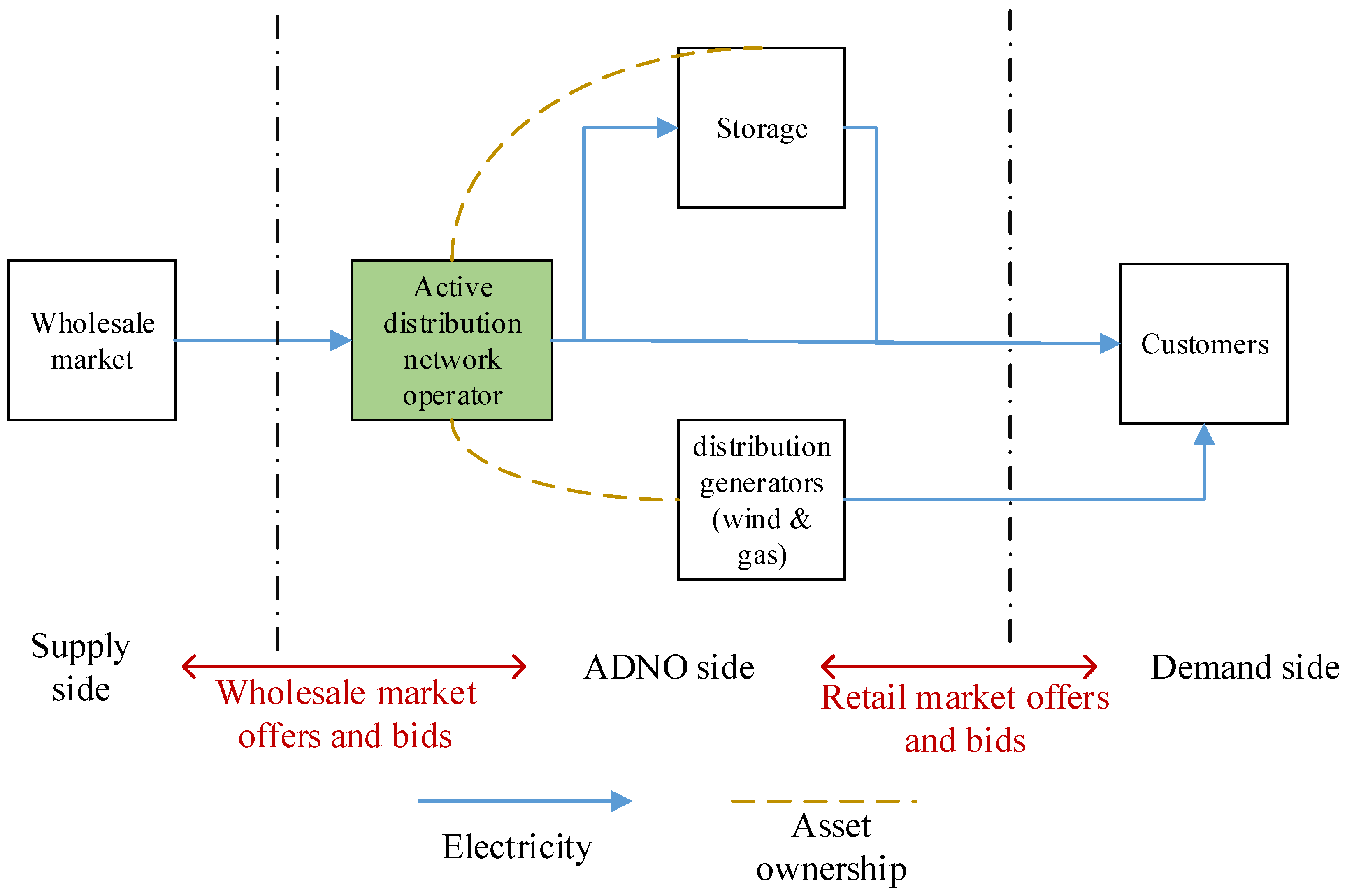
Figure 1. The basic operating model of ADNO.
Energies 16 04507 g001
Figure 2. Basic operating sequence of ADNO.
Energies 16 04507 g002
Figure 3. Pearson correlation coefficient between wind power generation and spot prices at different lag steps. (a) Shows the normalized value of wind output and day-ahead LMP; (b) shows the time-delay Pearson correlation coefficient between the two series.
Energies 16 04507 g003
Figure 4. Transformer neural network structure used in this paper.
Energies 16 04507 g004
Figure 5. The principle of the source embedding mechanism.
Energies 16 04507 g005
Figure 6. IEEE 33 test system used in this article.
Energies 16 04507 g006
Figure 7. Forecast performance comparison curve for a typical day. (a) is the result comparison of wind power forecast with and without source embedding; (b) is the result comparison of wind power forecast with and without conditioning; (c) is the result comparison of spot price forecast with and without source embedding; (d) is the result comparison of spot price forecast with and without conditioning.
Energies 16 04507 g007
Figure 8. Scheduling results on a typical day. (a) Is the dispatching result under 100% benchmark spot price; (b) is the dispatching result under 50% benchmark spot price.
Energies 16 04507 g008
Figure 9. The influence of subsidy level to E f f A D N O .
Energies 16 04507 g009
Figure 10. Sensitivity of ADNO’s profitability indicator E f f A D N O to wholesale market spot price levels.
Energies 16 04507 g010
Figure 11. Sensitivity of ADNO’s profitability indicator E f f A D N O to the elasticity coefficient of subsidies.
Energies 16 04507 g011
Figure 12. Sensitivity of the profitability indicator E f f A D N O of ADNO to wind power installed capacity.
Energies 16 04507 g012
Table 1. Hyperparameters and optimizer settings for models p 1 and p 2 .
Parameter NameParameter Size
Forecasting network batch size64
Transformer encoder block number2
Transformer decoder block number2
Transformer attention head number8
Input time series length72
Input featureShort-time Fourier transform (STFT)
Output time series length24
CBHGSame as in [32]
Source embedding training batch size64
optimizerAdam [32]
Learning rate0.001
Table 2. Comparison of the performance of our prediction method and traditional methods on the test set.
ModelTask1Task2
RMSE 1MAE 2RMSEMAE
LSTM [33]1.0030.8360.9090.840
CNN [33]0.7520.7530.7560.674
Seq2seq [34]0.6300.6160.5350.513
proposed0.5400.5530.4690.453
1 Root mean squared error. 2 Mean average error.
Table 3. The main hyperparameters of the deep neural network model used in this paper.
ParameterValue
Encoder input dimension72
Decoder input dimension24
Decoder output dimension24
Multi-head attention head number4
Number of encoder blocks2
Source embedding dimension128
Encoder output dimension128
Number of Decoder blocks2
Number of training batch48
Active functionTanh
Number of training epoch200
Training optimizerAdam
Initial learning rate5 × 10−5
Table 4. The baseline data used in this article.
ParameterValue
Network typeIEEE33
Total wind turbine capacity0.5 MW
Total energy storage capacity0.15 MWh
Total gas turbine capacity0.6 MW
Average variable cost of distributed gas power generation91 USD/MWh
Average start-up cost of distributed gas power generationUSD 20
Average demand SubsidyUSD 10
Average spot priceUSD 81/MWh
Table 5. Comparison of control variables for predictive effects.
Comparison FactorTest TaskRMSE 1
Without source embeddingtask10.621
Without conditioningtask10.594
Without source embeddingtask20.525
Without conditioningtask20.553
1 Root mean squared error.
Table 6. Comparison study of the proposed methods.
Model Comparison * E f f A D N O Value
With LSTM [33] forecast model2.209
With CNN [33] forecast model2.304
With Seq2seq [34] forecast model2.258
With proposed forecast model2.496
With single-level (no-subsidy) optimization [43]2.433
With proposed bi-level optimization2.496
* All settings are consistent with the baseline other than the comparison factor.
Disclaimer/Publisher’s Note: The statements, opinions and data contained in all publications are solely those of the individual author(s) and contributor(s) and not of MDPI and/or the editor(s). MDPI and/or the editor(s) disclaim responsibility for any injury to people or property resulting from any ideas, methods, instructions or products referred to in the content.