Optimization Study on Salinity Gradient Energy Capture from Brine and Dilute Brine

Abstract

The power conversion of salinity gradient energy (SGE) between concentrated brine from seawater desalination and seawater by reverse electrodialysis (RED) benefits energy conservation and also dilutes the discharge concentration to relieve the damage to coastal ecosystems. However, two key performance indexes of the maximum net power density and energy conversion efficiency for a RED stack harvesting the energy usually cannot reach the optimal simultaneously. Here, an optimization study on the two indexes was implemented to improve the performance of RED in harvesting the energy. A RED model for capturing the SGE between concentrated brine and seawater was constructed, and the correlation coefficients in the model were experimentally determined. Based on the model, the effects of a single variable (concentration, flow rate, temperature, thickness of the compartment, length of the electrode) on the performance of a RED stack are analyzed. The multi-objective optimization method based on the genetic algorithm was further introduced to obtain the optimal solution set, which could achieve the larger net power density and energy conversion efficiency with coordination. The ranges of optimal feed parameters and stack size were also obtained. The optimal flow velocity of the dilute solution and the concentration of the dilute solution are approximately 7.3 mm/s and 0.4 mol/kg, respectively.

1. Introduction

The availability of freshwater has decreased due to the persistent pollution and deterioration of freshwater resources. The available freshwater resources for human beings are less than one percent of global water resources [1]. Seawater desalination can effectively alleviate the current situation [2]. However, whether membrane desalination or thermal desalination discharges a large amount of concentrated brine and consumes amounts of energy as well is also of interest [3]. The direct discharge of the concentrated brine not only harms the surrounding marine organisms [4], but also wastes the salinity gradient energy (SGE), which is a chemical potential energy produced by mixing two kinds of electrolyte solutions with different concentrations, such as concentrated brine and seawater, or seawater and river water. As a sustainable green energy, the capture and conversion of the SGE has attracted much attention in recent years.

Methods of capturing the SGE include the ion exchange method [5], the osmotic method [6], the direct mixing method, the absorption method [7], and the vapor pressure difference method [8]. The osmotic and ion exchange methods are the most common methods. The osmotic method mainly refers to pressure retarded osmosis (PRO), which delays the osmotic flow through semipermeable membranes by applying hydrostatic back pressure to obtain pressure energy, and it can be further converted to electrical energy by hydraulic turbines [6]. The ion exchange method mainly includes reverse electrodialysis (RED), microbial reverse electrodialysis (MRED) [9], and accumulator-mediated mixing (ACCMIX) [10]. MRED is relatively complex with regard to equipment construction, operation and maintenance, and is limited by biological reactions. ACCMIX requires a greater amount of equipment, resulting in high operational complexity and additional energy loss during operation. However, the RED approach, with the advantages of a compact equipment structure, simple manufacturing process, and easy operation, is perfect for the capture and conversion of the SGE. It is based on the selective permeabilities of ion exchange membranes (IEMs) to anions and cations. The directional ion flow forms a series of potential differences on the IEMs, which promotes the oxidation-reduction reaction on the electrode plates in the RED stack and generates a current in the external circuit of the stack.

The RED began in 1954 [11], and 3.1 V of maximum voltage and 15 mW of power in a RED stack was acquired. In 1976, Weinstein and Leitz [12] increased the power density to 170 mW/m². Lacey [13] implemented an experimental study on several typical IEMs in 1980. However, the low selective permeabilities of the IEMs restricted the development of RED for a long period of time. With the in-depth study of IEMs, its performance has improved greatly in recent times. Vermaas [14] raised the power density to 2.2 W/m² by using the advanced IEMs and reducing the thickness of the compartments. Recently, applications of RED technology have been extended to different fields, such as a reverse electrodialysis heat engine [15,16], hydrogen production [17,18], the degradation of hexavalent chromium [19], and organic matter [20] in sewage, etc.

Feed solutions of the RED stack are mainly river water and seawater [21,22,23]. The low concentration of river water causes a large internal resistance which restricts the development of the capturing of the SGE between river water and seawater. Treatments of the concentrated brine have received significant attention, with a large number of seawater desalination plants put into operation [24]. However, the direct discharge of brine would have adverse effects on the survival of the surrounding marine organisms. Moreno et al. [4] found that the concentrated brine threatened the survival of seaweed, and the treatment of the concentrated brine by applying diffusers would greatly increase the operating cost. Drawing the concentrated brine and seawater into RED stacks not only reduces the direct discharge concentration of seawater desalination devices and efficiently reduces the damage to the marine ecology, but also obtains a significant amount of electric energy. We used the configured NaCl solutions with the same concentrations as concentrated brine and seawater as working fluids of the RED stack, and investigated the influences of feed parameters on the performances of the stack [25]. Furthermore, the parameter influences of natural seawater on a RED stack were experimentally analyzed, and a multi-stage RED system harvesting the SGE was also proposed [26]. In another study, the influences of trace ions in seawater on performances of the RED stack were experimentally analyzed [27]. In addition, influences of insoluble substances in natural seawater were experimentally studied, and it was found that the filtrated seawater (by smaller pore size) could enhance the performances of the RED stack [28]. Simulation studies on the influences of feed parameters were implemented, and the influences of stack sizes on stack performance were also explored [29,30].

Some scholars have investigated the performance optimization of the RED. Kim et al. [31] optimized the number of cell pairs using the experimental approach to increase net power and specific energy. Catarina et al. [32] used the method of electrical control to optimize the performance of multistage reverse electrodialysis. However, the algorithm is not used in the aforementioned studies. Michele et al. [33] adopted the gradient-ascent optimization algorithm to obtain the optimum thicknesses and velocities in the solution channels for different stack lengths and concentrations. Long et al. [34] used the non-dominated sorting genetic algorithm II to optimize the net power density and energy conversion efficiency of the stack. They [23] also adapted the genetic algorithm to investigate the effect of the compartment thickness on the performance of the RED stack and obtained the optimal compartment thickness. Furthermore, they studied the effects of the compartment thickness and the flow rate on the stack simultaneously, and obtained the optimal compartment thickness and flow rate. The optimization effect is better when the variables addressed simultaneously are changed from two to four in the process of performance optimization.

Through the above analysis, it was found that the critical performance indices of the RED stack (the max. net power density and the energy conversion efficiency) typically vary with feed parameters and stack sizes, and their maximum values cannot be acquired simultaneously, especially when seawater is used as the dilute solution of the stack. Therefore, the principal intention of this work is: (I) to comprehensively explore the performance of the RED stack under different feed parameters and stack sizes; and (II) to optimize the feed parameters and stack sizes comprehensively in order to obtain the optimum feed parameters and stack sizes in which the max. net power density and the energy conversion efficiency can be coordinated. Based on the aforementioned purposes, a model that enables the simultaneous addressing of multiple variables was constructed with correlation coefficients determined through experimentation. Secondly, the multi-objective optimization based on a genetic algorithm is introduced to obtain the optimum feed parameters and stack sizes with max. net power density and energy conversion efficiency as the objective functions. This study could provide the optimal parameters in designing stack sizes and adjusting the feed parameters for a RED stack to achieve a coordinated performance of the max. net power density and the energy conversion efficiency.

2. Methods and Experimental Verifications

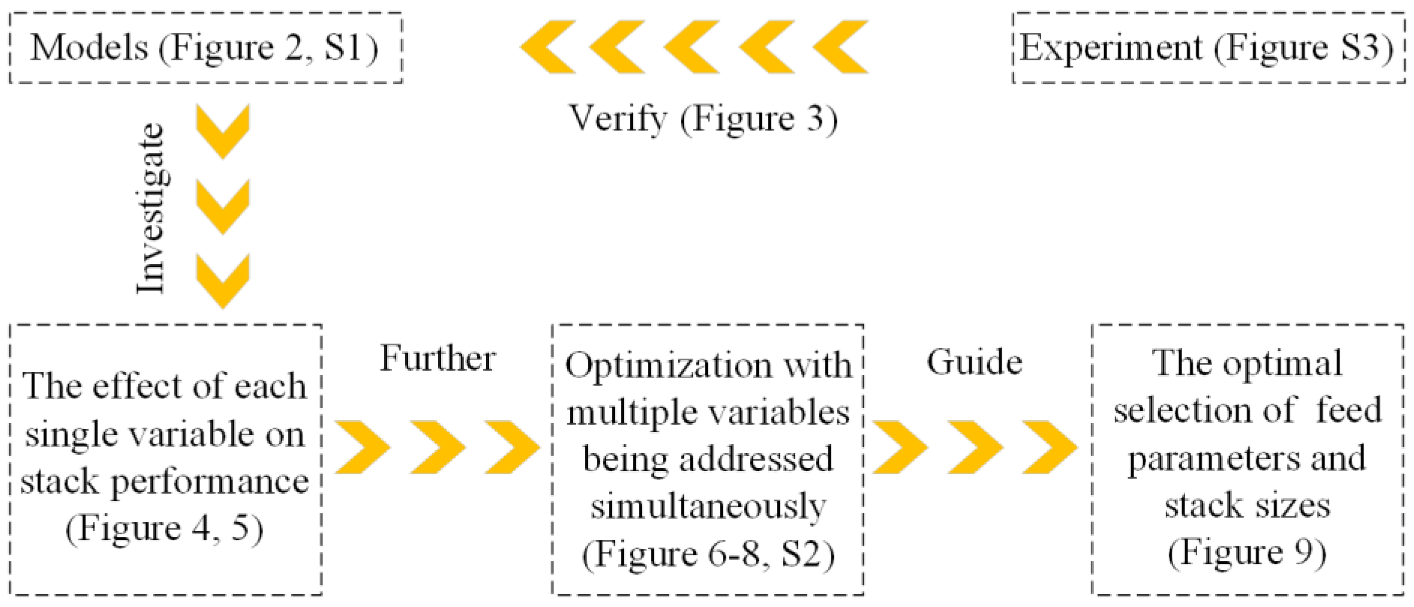
A flowchart of the methodology is shown in Figure 1. First, a theoretical model was established (Figure 2 and Figure S1), and the relevant coefficients and model accuracy were verified by experiments (Figure 3 and Figure S3). Secondly, the influence of single variables (concentration, flow rate, temperature, compartment thickness, and electrode plate length) on the performance of the stack was studied with the aid of the constructed model (Figure 4 and Figure 5). Finally, based on the effects mentioned above, a multi-objective optimization was carried out based on the genetic algorithms (Figure 6, Figure 7, Figure 8 and Figure S2) to provide a reference for the optimal feed parameter selection and stack size design (Figure 9).

2.1. Models

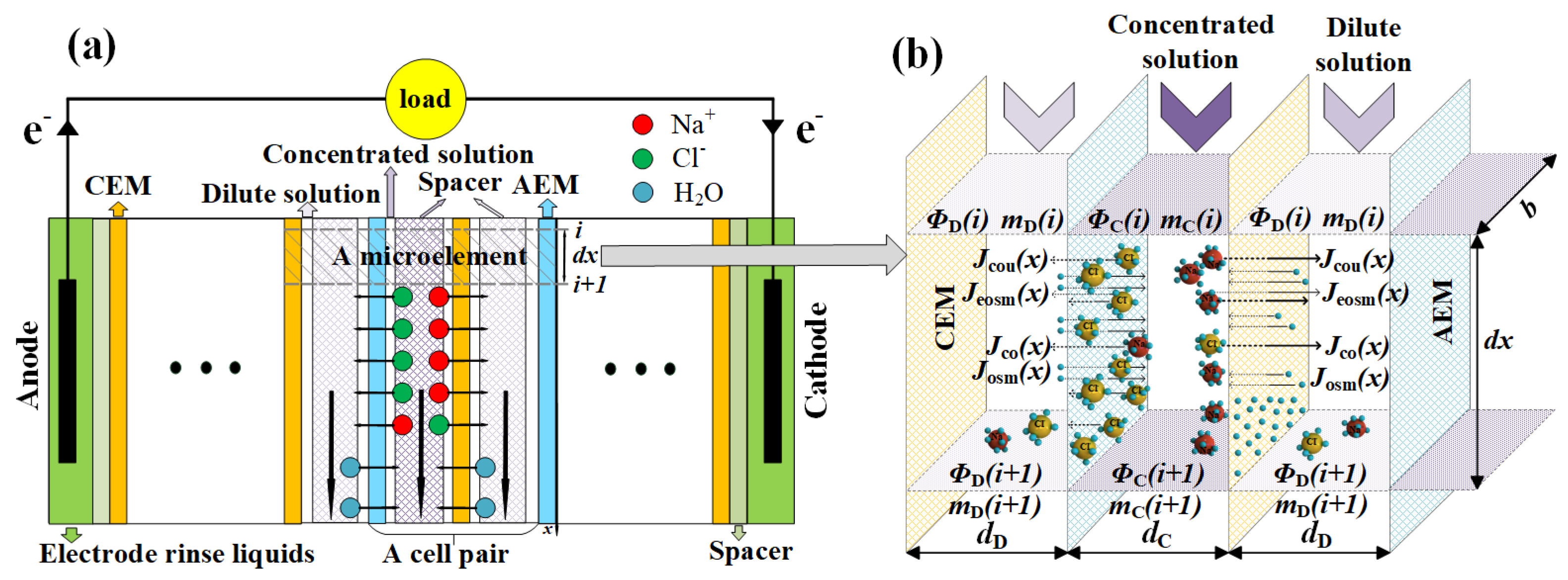
2.1.1. Ion Migration Models of a RED Stack

Figure 2a shows the working principle of a RED stack, which is mainly composed of ion exchange membranes (IEMs), compartments, electrodes, and separating spacers. When feed solutions flow along the channel direction, Na⁺ and Cl⁻ ions in the concentrated solution migrate to the dilute solutions through cation exchange membranes (CEMs) and anion exchange membranes (AEMs), respectively. The directional migration of ions forms a series of potential differences between IEMs, an oxidation-reduction reaction finally occurs at the electrodes, and a current is generated in the external circuit. A RED stack is stacked by many identical cell pairs, and a cell pair is composed of an AEM, a CEM, a concentrated solution compartment, a dilute solution compartment, and two spacers. A cell pair is divided into finite microelements along the flow direction when constructing migration models of ions. The distributed parameters model is introduced to construct ion migration in each microelement. The migration models in a microelement are shown in Figure 2b. It is assumed that the inlet of feed solutions is the origin of the x-axis, and the flow direction along the channel is regarded as the positive direction. According to the Nernst equation [35], the electromotive force of a cell pair generated at position x can be expressed as

$$E_{\mathrm{cell}}(x)={\alpha }_{\mathrm{CEM}}\frac{\mathrm{R}T}{z\mathrm{F}}\ln (\frac{{\gamma }_{\mathrm{C}}^{{\mathrm{Na}}^{+}}(x)c_{\mathrm{C}}^{{\mathrm{Na}}^{+}}(x)}{{\gamma }_{\mathrm{D}}^{{\mathrm{Na}}^{+}}(x)c_{\mathrm{D}}^{{\mathrm{Na}}^{+}}(x)})+{\alpha }_{\mathrm{AEM}}\frac{\mathrm{R}T}{z\mathrm{F}}\ln (\frac{{\gamma }_{\mathrm{C}}^{{\mathrm{Cl}}^{-}}(x)c_{\mathrm{C}}^{{\mathrm{Cl}}^{-}}(x)}{{\gamma }_{\mathrm{D}}^{{\mathrm{Cl}}^{-}}(x)c_{\mathrm{D}}^{{\mathrm{Cl}}^{-}}(x)})$$

(1)

where R is the gas constant, T is the Kelvin temperature, z is the ionic valence, F is the Faraday constant, γ is the average ionic activity coefficient of a solution, and c is the concentration.

The open circuit voltage (OCV) of a RED stack can be expressed as:

$$OCV=N\cdot E_{\mathrm{cell}}{|}_{(x=L)}$$

(2)

where N is the number of cell pairs in a RED stack. In Equation(1), the calculations of ${\alpha }_{\mathrm{CEM}}$ and ${\alpha }_{\mathrm{AEM}}$ are listed in

Table 1. Calculations of ${\alpha }_{\mathrm{CEM}}$ and ${\alpha }_{\mathrm{AEM}}$.

Descriptions	Formulas	Unit
Effective selective permeability coefficient of AEM	${\alpha }_{\mathrm{AEM}}=\beta {\alpha }_{\mathrm{AEM}}^0$	-
Effective selective permeability coefficient of CEM	${\alpha }_{\mathrm{CEM}}=\beta {\alpha }_{\mathrm{CEM}}^0$	-
Correction factor	$\beta ={\beta }_1+{\beta }_2{c}_{\mathrm{D}}(x)+{\beta }_3{c}_{\mathrm{C}}(x)$	-

,where ${\alpha }_{\mathrm{AEM}}^0$ and ${\alpha }_{\mathrm{CEM}}^0$ are nominal selective transmission coefficients of AEM and CEM, respectively. $\beta$ is the correction factor of the selective permeability coefficient. The values of ${\beta }_1$, ${\beta }_2$ and ${\beta }_3$ in Table 1 are 1.0196, 0.0347, and −0.0448, respectively [36].

The inner resistance at position x(r(x)) is the series resistance of the ion exchange membranes resistance (r_CEM and r_AEM), the resistance of the electrodes ($r_{\mathrm{el}}$), the resistance of the dilute solution compartment (r_D), and concentrated solution compartment resistance (r_C). It can be expressed as

$$r(x)=N[r_{\mathrm{C}}(x)+r_{\mathrm{D}}(x)+r_{\mathrm{CEM}}(x)+r_{\mathrm{AEM}}(x)]+r_{\mathrm{el}}(x)$$

(3)

The resistances in Equation(3) can be calculated by solving the equations in

Table 2. The calculation of resistances.

Descriptions	Formulas	Unit
Resistance of the concentrated compartment	$r_{\mathrm{C}}(x)=f_{\mathrm{y}}\frac{d_{\mathrm{C}}}{{\Lambda }_{\mathrm{C}}(x)c_{\mathrm{C}}(x)}$ [36]	Ω·m2
Resistance of the dilute compartment	$r_{\mathrm{D}}(x)=f_{\mathrm{y}}\frac{d_{\mathrm{D}}}{{\Lambda }_{\mathrm{D}}(x)c_{\mathrm{D}}(x)}$ [36]	Ω·m2
Correction factor	$f_{\mathrm{m}}=f_{\mathrm{m},1}+f_{\mathrm{m},2}{c}_{\mathrm{D}}(x)+f_{\mathrm{m},3}{c}_{\mathrm{C}}(x)$ [36]	-
Resistance of AEM	$r_{\mathrm{AEM}}(x)=f_{\mathrm{m}}{r}_{\mathrm{AEM}}^0$ [36]	Ω·m2
Resistance of CEM	$r_{\mathrm{CEM}}(x)=f_{\mathrm{m}}{r}_{\mathrm{CEM}}^0$ [36]	Ω·m2

. The inner resistance of an RED stack can be expressed as

$$r=\frac{OCV-U}{I}$$

(4)

where r is the resistance of a stack, U is the output voltage of a stack, and I is the output current of a stack.

In Table 2, $f_{\mathrm{y}}$ is the shielding coefficient of the spacer, and its value is 1.5625 [37]. Λ is the molar conductivity, d_C is the thickness of the concentrated solution compartment, and d_D is the thickness of the dilute solution compartment. $f_{\mathrm{m}}$ is the correction factor of IEMs, which changes with the concentration of feed solutions. The value of $f_{\mathrm{m},1}$, $f_{\mathrm{m},2}$, and $f_{\mathrm{m},3}$ is 2.4541, 0.026, and 0.0312, respectively [36].

In the RED stack, ions in the concentrated solution migrate through IEMs. The ion flux at position x can be expressed as

$$J_{\mathrm{tot}}(x)=J_{\mathrm{cou}}(x)+J_{\mathrm{co}}(x)=\frac{j(x)}{\mathrm{F}}+\frac{2D{c}_{\mathrm{Nacl}}}{d_{\mathrm{IEM}}}[c_{\mathrm{C}}(x)-c_{\mathrm{D}}(x)]$$

(5)

where, J_cou is the cou-ion molar flux, J_co is the co-ion molar flux, and d_IEM is the thickness of the IEM. $D{c}_{\mathrm{NaCl}}$ is the diffusion coefficient of IEMs for NaCl, with the value of 1 × 10⁻¹² m²/s [38]. The current density $j(x)$ can be acquired by the following equation.

$$j(x)=\frac{N\cdot E_{\mathrm{cell}}(x)-U}{r(x)}$$

(6)

Water molecules also permeate IEMs due to the concentration difference. Moreover, the carrying effect of ions in the migration process also causes the permeation of water molecules. For of the effects, the transport of water molecules can be expressed as

$$J_{\mathrm{w}}(x)=J_{\mathrm{osm}}(x)-J_{\mathrm{eosm}}(x)=2L_{\mathrm{p}}\upsilon RT[{\phi }_{\mathrm{C}}{c}_{\mathrm{C}}(x)-{\phi }_{\mathrm{D}}{c}_{\mathrm{D}}(x)]-n_{\mathrm{h}}{J}_{\mathrm{tot}}(x)$$

(7)

where, J_osm is the osmosis flux, J_eosm is the electroosmosis flux, L_p is the permeability coefficient of the ion exchange membranes to water, $\upsilon$ is the number of ions in the solution of one mole of solute, and φ is the osmotic coefficient of water. $n_{\mathrm{h}}$ is the number of water molecules carried by an ion, with the value of 7 for a Na⁺ or Cl⁻ [36].

Due to the lateral migrations of ions and water molecules across IEMs, the volume flow, density, and molar concentration of the concentrated solution will change, which can be expressed by the difference equation [29]:

$$\frac{d[{\Phi }_{\mathrm{C}}(x){\rho }_{\mathrm{C}}(x)]}{dx}=-b{J}_{\mathrm{tot}}(x)M_{\mathrm{NaCl}}+b{J}_{\mathrm{w}}(x)M_{{\mathrm{H}}_2\mathrm{O}}$$

(8)

The differential equation of concentration in the concentrated solution

$$\frac{d[{\Phi }_{\mathrm{C}}(x)c_{\mathrm{C}}(x)]}{dx}=-b{J}_{\mathrm{tot}}(x)$$

(9)

The differential equation of density in the dilute solution

$$\frac{d[{\Phi }_{\mathrm{D}}(x){\rho }_{\mathrm{D}}(x)]}{dx}=b{J}_{\mathrm{tot}}(x)M_{\mathrm{NaCl}}-b{J}_{\mathrm{w}}(x)M_{{\mathrm{H}}_2\mathrm{O}}$$

(10)

The differential equation of concentration in the dilute solution

$$\frac{d[{\Phi }_{\mathrm{D}}(x)c_{\mathrm{D}}(x)]}{dx}=b{J}_{\mathrm{tot}}(x)$$

(11)

where ρ is the density, M is the molar mass, Φ is the volume flow of solution, and b is the width of compartments.

The performances of a RED stack can be obtained by integrating the above equations in all microelements, and the principal evaluation indexes of a RED stack are listed in

Table 3. Performance evaluation indexes of a RED stack.

Descriptions	Formulas	Unit
Output current	$I=b{\displaystyle {\int }_0^{L}j(x)dx}$	A
Gross power	$P_{\mathrm{g}}=UI$	W
Power loss	$P_{\mathrm{P}}=\Delta P{r}_{\mathrm{C}}{\Phi }_{\mathrm{C}}+\Delta P{r}_{\mathrm{D}}{\Phi }_{\mathrm{D}}$	W
Pressure loss in concentrated solution compartment	$\Delta P{r}_{\mathrm{C}}=\frac{12{\mu }_{\mathrm{C}}L{\Phi }_{\mathrm{C}}}{b{d}_{\mathrm{C}}^3}$	Pa
Pressure loss in dilute solution compartment	$\Delta P{r}_{\mathrm{D}}=\frac{12{\mu }_{\mathrm{D}}L{\Phi }_{\mathrm{D}}}{b{d}_{\mathrm{D}}^3}$	Pa
Net power	$P_{\mathrm{n}}=P_{\mathrm{g}}-P_{\mathrm{P}}$	W
Gross power density	$P_{\mathrm{A}}=\frac{P_{\mathrm{g}}}{A_{\mathrm{RED}}}$	W/m2
Net power density	$P_{\mathrm{An}}=\frac{P_{\mathrm{n}}}{A_{\mathrm{RED}}}$	W/m2
Energy conversion efficiency	$\eta =\frac{P_{\mathrm{g}}}{\Delta G_{\max }}$	-
Maximum Gibbs free energy	$\Delta G_{\max }=2RT[{\Phi }_{\mathrm{C}}{c}_{\mathrm{C}}\ln \frac{c_{\mathrm{C}}}{c_{\mathrm{M}}}+{\Phi }_{\mathrm{D}}{c}_{\mathrm{D}}\ln \frac{c_{\mathrm{D}}}{c_{\mathrm{M}}}]$	W

, where μ is the dynamic viscosity and A is the area. The calculation process is illustrated in Figure S1. Among them, difference Equations (8)–(11) are simultaneously solved by the R-K method.

2.1.2. Optimization Models of a RED Stack

The performances of the RED stack can be predicted by applying the above models. However, Max. P_An and $\eta$ cannot simultaneously reach the maximum value under different operating conditions. Therefore, both of them are determined as objective functions in the optimization models. According to the format requirements of the genetic algorithm, the Max. P_An and η should take a negative value, and then the minimum value is obtained. Thus, the multi-objective function can be expressed by Equations (12) and (13). According to the performance analysis, the constraints of the working condition requirements of IEMs and the discharge parameters of thermal seawater desalination are described by Equation(14). The multi-objective optimization model is illustrated in Figure S2.

$$\mathrm{Min}. (\mathrm{Max}. P_{\mathrm{An}})=-f(m_{\mathrm{C}},m_{\mathrm{D}},t,v_{\mathrm{C}},v_{\mathrm{D}},d_{\mathrm{C}},d_{\mathrm{D}},L)$$

(12)

$$\mathrm{Min}. (\eta )=-f(m_{\mathrm{C}},m_{\mathrm{D}},t,v_{\mathrm{C}},v_{\mathrm{D}},d_{\mathrm{C}},d_{\mathrm{D}},L)$$

(13)

$$\{\begin{array}{l}{m}_{\mathrm{C},\min }\le m_{\mathrm{C}}\le m_{\mathrm{C},max}\\ m_{\mathrm{D},min}\le m_{\mathrm{D}}\le m_{\mathrm{D},\max }\\ t_{\min }\le t\le t_{\max }\\ v_{\mathrm{C},\min }\le v_{\mathrm{C}}\le v_{\mathrm{C},\max }\\ v_{\mathrm{D},\min }\le v_{\mathrm{D}}\le v_{\mathrm{D},\max }\\ d_{\mathrm{C},\min }\le d_{\mathrm{C}}\le d_{\mathrm{C},\max }\\ d_{\mathrm{D},\min }\le d_{\mathrm{D}}\le d_{\mathrm{D},\max }\\ L_{\min }\le L\le L_{\max }\end{array}$$

(14)

where m is the mass molar concentration, t is the temperature, v is the velocity of feed solution, d is the thickness of the compartment, and L is the length of the electrodes. The subscript “C” represents the concentrated solution, and “D” represents the dilute solution.

2.2. Experiment

To verify the accuracies of the models, a RED experiment is constructed in Figure S3a. Specifications and quantities of the main instruments are listed in Table S1. Figure S3b shows a physical view of the RED stack, and its constituent components are listed in Table S2. The concentrated solution flows into the stack from the inlet (A) and is discharged from the outlet (D) after accomplishing the ions exchange. The dilute solution flows into the stack from the inlet (G) and is discharged from the outlet (C) after completing the ions exchange. The electrode rinsing liquid enters the electrode chamber from the inlet (E) and is discharged from the outlet (F) after the oxidation-reduction reaction is completed in the electrode chamber. Compared to heterogeneous IEMs, homogeneous IEMs have the advantages of low resistance and a high ion exchange capacity [5,39]. Therefore, the homogeneous IEMs produced by Fuji are used in the experiment, and their principal performance is listed in Table S3. The inert iridium ruthenium titanium electrode is used as the anode and cathode, and the electrode rinsing solutions are the mixed solutions of ${\mathrm{K}}_4{\mathrm{Fe}\left(\mathrm{CN}\right)}_6$, ${\mathrm{K}}_3{\mathrm{Fe}\left(\mathrm{CN}\right)}_6$, and NaCl [40]. The cathodic reaction can be expressed as ${\mathrm{Fe}\left(\mathrm{CN}\right)}_6^{3^{-}}{+\mathrm{e}}^{-}\to {\mathrm{Fe}\left(\mathrm{CN}\right)}_6^{4^{-}}$, and the anodic reaction is ${\mathrm{Fe}\left(\mathrm{CN}\right)}_6^{4^{-}}-{\mathrm{e}}^{-}\to {\mathrm{Fe}\left(\mathrm{CN}\right)}_6^{3^{-}}$. The experimental steps are detailed in the reference [25], and it is no longer described here.

2.3. Model Verification

To verify the accuracy of the performance model of the RED stack, the experiments are carried out when m_C is 1.0 mol/kg, 1.5 mol/kg and 2.0 mol/kg, respectively. In the experimental process, the feed temperature (t) is kept at 35 °C, both v_C and v_D are 8.7mm/s, and m_D is set as 0.6mol/kg. The comparisons between experimental and simulation results are shown in Figure 3. Figure 3a shows the variation of U with I. When I is close to zero, U is equal to OCV. When m_C is 1.0 mol/kg, 1.5 mol/kg and 2.0 mol/kg, respectively, the tested OCV is 0.205 V, 0.364 V, and 0.466 V, respectively, and the simulation value is 0.207 V, 0.359 V, and 0.457 V, with errors of 0.97%, 1.37%, and 1.93%, respectively. It also can be observed that the measured internal resistance (r) of the stack is 5.88 Ω, 5.13 Ω, and 4.04 Ω, respectively, and the simulation values are 5.84 Ω, 5.13 Ω, and 3.93 Ω, with errors of 0.69%, 0, and 2.7%, respectively. Figure 3b shows the variations of P_A with U. The Max. P_A measured in the experiment is 23.1 mW/m², 79.4 mW/m², and 17.1 mW/m², respectively. The simulation values are 23.7 mW/m², 81.7 mW/m², and 17.2 mW/m², with errors of 2.59%, 2.89%, and 0.58%, respectively. It can be concluded that the maximum error between the simulation and the experiment is less than 3% by comparing Figure 3a, b, which shows the performance prediction models with good accuracy.

3. Results and Analysis

3.1. Influences of Feed Parameters and Stack Sizes on Performances of a RED Stack

The discharge concentration of brine from the thermal seawater desalination plants is in the general range of 1.0 mol/kg–1.5 mol/kg, and the concentration of natural seawater is generally in the range of 0.5 mol/kg–0.6 mol/kg. Therefore, m_C and m_D are set in the range of 1.0 mol/kg–2.0 mol/kg NaCl solution, and 0.4 mol/kg–0.6 mol/kg NaCl solution in the simulation program. The performances of the stack can be reflected by OCV, Max. P_An (maximum net power density) and η (energy conversion efficiency), as shown in Figure 4. Here, η and U respectively refer to the energy conversion efficiency and the corresponding voltage at the max. P_A. Figure 3a–c reveal the effects of m_C and m_D on OCV, the Max. P_An and η under the conditions of 35 °C of t, 8.7 mm/s of v_C, 8.7 mm/s of v_D, 0.118 m of L, 0.065 m of b, 0.3 mm of d_C, and 0.3 mm of d_D.

Figure 4a shows that OCV increases with the increase of m_C and decreases with the increase of m_D. With the increase of m_C, the slope of the isolines in the figure gradually decreases, which indicates that m_D has a more obvious influence on OCV than m_C when m_C is relatively large. According to Equation (1), a greater ratio of m_C and m_D can reach a larger OCV. After the concentration of the solution reaching a certain value, if the concentration continues to increase, a large amount of ion pairs will form in the solution, which will reduce the OCV. Figure 4b shows that the max. P_An of the stack increases with the increase of m_C and decreases with the increase of m_D. The slope of the isolines in the figure gradually decreases, which indicates that m_D has a greater impact on Max. P_An than m_C when m_C is relatively large. P_An can reach 225 mW/m². With the increase of m_C, OCV and U increase, and the amount of free ions in the concentrated solution increases, the conductivity increases, R_i decreases, and thus P_An increases. With the decrease of m_D, the amount of free ions in the dilute solution decreases, the conductivity decreases, and R_i increases. However, the contribution of the U increment to the Max. P_An is greater than R_i, so Max. P_An will increase. Figure 4c shows that η is increased with the decrease of m_C and m_D. When m_C increases, P_A increases, and the SGE entering the stack increases. However, the influence of the max. P_A increment is less than that of the SGE increment, so η is decreased. When m_D decreases, Max. P_A increases, and the SGE also increases. The influence of the max. P_A increment is greater than that of the SGE increment, so η is improved.

Figure 3d–f reveal the influences of v_C and v_D on the performances of the stack under the conditions of 35 °C of t, 0.118 m of L, 0.065 m of b, 0.3 mm of d_C, 0.3 mm of d_D, 2 mol/kg of m_C, and 0.6 mol/kg of m_D. Figure 4d shows that OCV increases rapidly with the increase of v_D at low v_C, and remains unchanged when v_D reaches a critical value. The critical value increases correspondingly with the increase of v_C. This is because the concentration at the inlet and outlet of the solution changes greatly at a low v_C and v_D, resulting in a small concentration difference at the outlet, which causes serious electrodialysis. With the increase of v_D, the concentration difference at the outlet increases, so OCV will increase. However, when v_D continues to increase after reaching the critical value, the OCV will tend to be stable. This is due to the factor restricting the continuous increase of OCV no longer being restricted by the flow rate, but rather the selective permeability of the IEMs. Figure 4e shows that Max. P_An is increased with the increase of v_C and v_D. It can be found that Max. P_An increases first and then decreases with the increase of v_D at a medium flow rate of the concentrated solution. This is caused by the large flow loss. The max. P_An in the figure can reach 155 mW/m². Figure 4f shows that η is generally decreased with the increase of v_C and v_D. When v_C is relatively small, such as less than 3.0 mm/s, with the increase of v_D, η is increased first and then decreased. This is due to the serious electrodialysis phenomenon at low v_D. At this time, the flow rate is the principal constraint factor of η, so it is increased with the increase of v_D. At high v_D, increasing the flow rate can increase P_g, but the influence of the P_g increment is less than that of the SGE increment, so η is decreased. The contour lines in Figure 4f are not completely symmetrical, and the concave surface is slightly inclined to the v_D axis, which indicates that the impact of v_C on η is larger than v_D in general.

Figure 4g–i reflect the effects of compartment thickness (d_C and d_D) on OCV, max. P_An, and η under the conditions of 35 °C of t, 0.118 m of L, 8.7 mm/s of v_C, 8.7 mm/s of v_D, 2.0 mol/kg of m_C, and 0.6 mol/kg of m_D. At low d_C and d_D, the effect of compartment thickness on OCV and max. P_An is obvious (Figure 4g,h). This is because with the increase in d_C and d_D, the volume flow of the feed solution increases, the concentration variations of the feed solutions decrease along the flow channel, and the concentration difference at the outlet becomes larger, and therefore OCV and max. P_An become larger. At high d_C and d_D, the main factor restricting the increase of OCV and Max. P_An is no longer the compartment thickness, but rather than the selective permeability of IEMs and the solution concentration. The maximum OCV and Max. P_An in Figure 4g,h can reach 0.51 V and 180 mW/m², respectively. Oppositely, the variation trend of η is opposite to OCV and max. P_An with the variations of d_C and d_D (Figure 4i). With the thickness of the compartment increasing, the volume flow rate increases, which means an increase in SGE. However, the increment of P_g is less than the increment of SGE, so η decreases.

In Figure 5a, L =0.118m, b =0.065m, v_C = 8.7 mm/s, v_D = 8.7 mm/s, m_C = 2 mol/kg, m_D = 0.6 mol/kg, d_C = 0.3 mm, and d_D = 0.3 mm. In Figure 5b, t =35 °C, b =0.065m, v_C = 8.7 mm/s, v_D = 8.7 mm/s, m_C = 2 mol/kg, m_D=0.6 mol/kg, d_C = 0.3 mm, and d_D = 0.3 mm.

Figure 5 shows the effects of t and L on the performance of the RED stack. It is shown in Figure 5a that max. P_An, OCV, and η are increased with the increase of t. The free ions in the solutions become more active with the rise of t, the migration amount of the ions increases, and the potential difference on both sides of the IEMs increases, which causes the increase of OCV. The conductivity of the solution is also enhanced with the increase of t, and R_i is decreased, so P_g is increased and Max. P_An is increased. The SGE entering the RED stack increases; however, the increment of SGE is smaller than the increment of max. P_An, so η is improved. Figure 5b shows that max. P_An and OCV are decreased with the increase of L, but η is increased. The concentration difference at the outlet decreases with the increase of L, so OCV and U are decreased (Equation (2)). The increment of I to max. P_An is smaller than that of the U decrease, so max. P_An decreases with the increase of L. The flow loss also increases with the increase of L, so max. P_An is further reduced. η is improved due to the fact that SGE entering the stack remains unchanged. The max. P_An in Figure 5b can reach 173 mW/m², and η can reach up to 2.77%. It was concluded that the feed solution concentration has the most significant effect on the maximum net power density of the stack, and the flow velocity and the length of the electrode plate have the most obvious effect on the energy conversion efficiency of the stack.

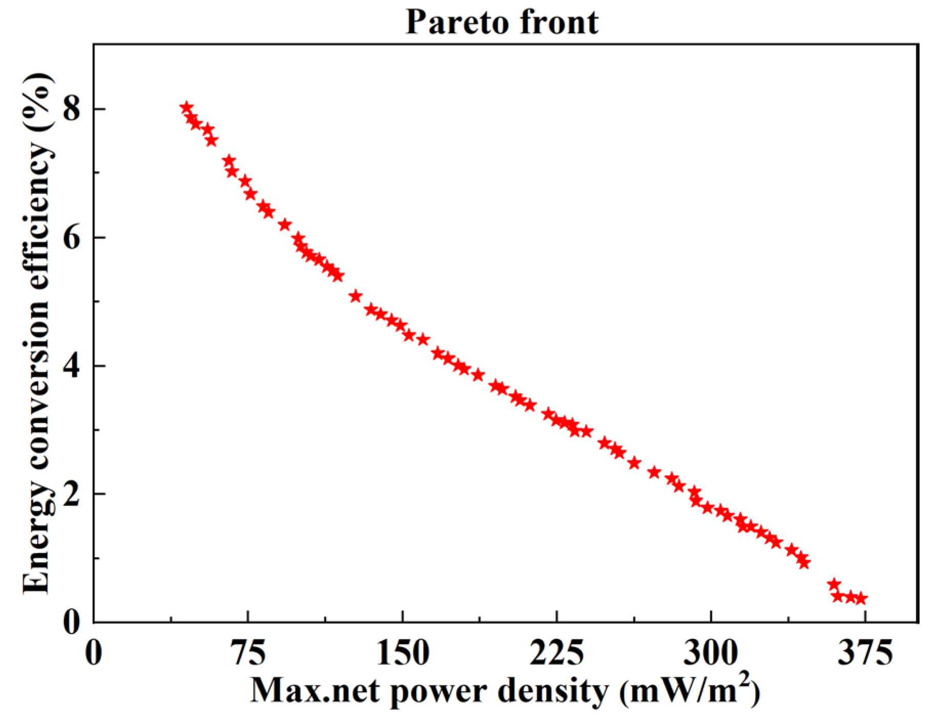
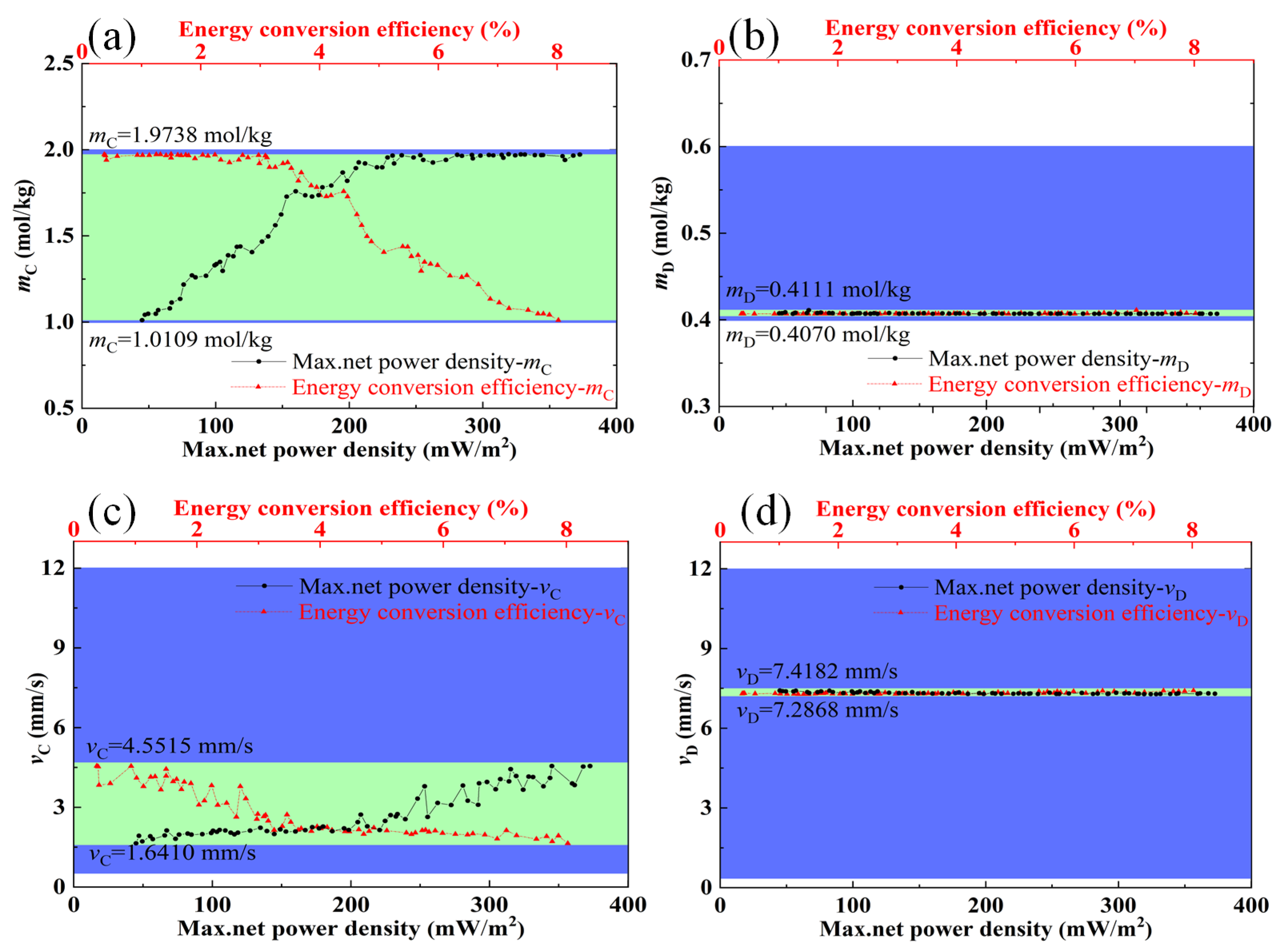
3.2. Optimization Analysis

According to the above analysis, it was found that it is difficult to achieve the maximum values of the max. P_An and η simultaneously. Therefore, the multi-objective optimization based on the genetic algorithm is introduced to obtain the Pareto frontier coordinating the Max. P_An and η. The ranges of values of each of the independent variables are listed in

Table 4. Feed parameters and stack sizes.

Parameters	mC (mol/kg)	mD (mol/kg)	t (°C)	vC (mm/s)	vD (mm/s)	dC (mm)	dD (mm)	L (m)
Upper limit	2.0	0.6	70	12.0	12.0	2.0	2.0	1.00
Lower limit	1.0	0.4	25	0.5	0.5	0.1	0.1	0.05

. The corresponding P_An and η are obtained by the model calculation when these variables take specific values, which is called a solution of the independent variables. The set of solutions of the independent variables caused by these variables is huge. The Pareto frontier, i.e., an optimal set of solutions, is obtained via the above algorithm. For any solution A in the independent variable solution set, a solution B can always be found in the optimal solution set in which the Max. P_An and η are both greater than that in A. The Pareto front is shown in Figure 6.

Further analysis of the optimal solution set is required in order to find the optimal feed parameters and stack sizes in which the max. P_An and η can be coordinated. The results of the analysis are shown in Figure 7 and Figure 8.

The optimal ranges of variables in which max. P_An and η can achieve coordination are shown in Figure 7. The blue area in the figure is the set range, and the green area is the optimal range derived based on the optimal solution set. Figure 7a–d show the optimal ranges of m_C, m_D, v_C, and v_D when max. P_An and η achieve reconciliation. The upper limits of the ranges are 1.9738 mol/kg, 0.4111 mol/kg, 4.5515 mm/s, and 7.4182 mm/s, respectively. The lower limits are 1.0109 mol/kg, 0.4070 mol/kg, 1.6410 mm/s, and 7.2868 mm/s, respectively. It was found that the overall trend of the optimal m_C and v_C (Figure 7a,c) changes are increased with the increase of max. P_An, and decreasing m_C and v_C can raise η. It is worth noting that the optimal ranges of m_D and v_D (Figure 7b,d) are relatively narrow, which guides the selection of the feed parameters.

The optimal ranges of variables in which max. P_An and η can achieve coordination are shown in Figure 8. Figure 8a–d show the optimal ranges of d_C, d_D, L, and t when max. P_An and η achieve coordination. The upper limits of the ranges are 0.7437 mm, 0.9437 mm, 0.8864 m, and 69.1 °C, respectively. The lower limits are 0.3306 mol/kg, 0.5808 mol/kg, 0.0582 m, and 62.5 °C, respectively. Figure 8a shows that d_C increases overall with the increase of max. P_An, but decreases with the increase of η. The overall trend of d_D (Figure 8b) with max. P_An and η is opposite to that of d_C. L (Figure 8c) decreases overall with increasing max. P_An and increases with increasing η. It is worth noting that the optimal range of t is relatively narrow, which guides the selection of the feed parameters. The reasons of the overall trends of m_C, m_D, v_C, v_D, d_C, d_D, L, and t (Figure 7 and Figure 8) with max. P_An and η are referred to in Section 3.1. However, the reference is not accurate because the results in Section 3.1 are based on a univariate analysis. In contrast, in this section the above results are caused by eight variables that are addressed simultaneously by the multi-objective optimization method based on the genetic algorithm.

Figure 9a reflects the variation of optimal power density and energy conversion efficiency with the concentration of the concentrated solution, as well as the variation of solution feeding parameters (Figure 9b) and the optimal stack size (Figure 9c) when the RED stack achieves optimal performance. As m_C increases, the optimal v_C and d_C increase, and the optimal L and d_D decrease, while the optimal v_D, t, and m_D remain almost unchanged. This indicates that, regardless of the variation of m_C within the range of 1.0–2.0 mol/kg, the maximum power density and energy conversion efficiency of the stack can be achieved simultaneously when v_D, t, and m_D are around 7.3 mm/s, 66 °C, and 0.4 mol/kg, respectively. Due to the fact that the concentration of the concentrated brine discharged by the thermal seawater desalination device is generally two to three times the concentration of seawater, the optimal feed parameters and stack size can be selected to coordinate the maximum power density and energy conversion efficiency of the stack, and achieve a higher value, as shown in Figure 9.

4. Conclusions

The effects of single variables in feed parameters and stack sizes on stack performance are investigated comprehensively by the constructed model, in which the correlation coefficients are determined by experiments. Furthermore, a multi-objective optimization method based on the genetic algorithm is introduced to address these variables simultaneously in order to obtain an optimal solution set that can achieve the larger net power density and the energy conversion efficiency with coordination. The principal conclusions are as follows:

(1)

The concentration of feed solutions has the most significant effect on the maximum net power density of the stack, whereas the flow velocity and the length of the electrode plate have the most obvious effect on the energy conversion efficiency of the stack.

(2)

The optimal ranges of feed parameters (concentration, flow velocity, and temperature) and stack sizes (the compartment thickness and the length of electrode plate) were obtained, in which the maximum net power density and energy conversion efficiency could be coordinated and relatively larger. The optimal ranges of the flow velocity of the concentrated solution and feed solution temperature are 1.6 mm/s,−4.6 mm/s, and 62–69 °C, respectively.

(3)

The optimal compartment thickness and the length of the electrode plate are obtained based on the discharge concentration of concentrated seawater from different desalination plants. The maximum net power density and energy conversion efficiency can be coordinated when the flow velocity of the dilute solution and the concentration of the dilute solution are approximately 7.3 mm/s and 0.4 mol/kg, respectively.

References

1. Baggio, G.; Qadir, M.; Smakhtin, V. Freshwater availability status across countries for human and ecosystem needs. Sci. Total Environ. 2021, 792, 148230. [Google Scholar] [CrossRef]
2. Prajapati, M.; Shah, M.; Soni, B.; Parikh, S.; Sircar, A.; Balchandani, S.; Thakore, S.; Tala, M. Geothermal-solar integrated groundwater desalination system: Current status and future perspective. Groundw. Sustain. Dev. 2021, 12, 100506. [Google Scholar] [CrossRef]
3. Amy, G.; Ghaffour, N.; Li, Z.; Francis, L.; Linares, R.; Missimer, T.; Lattemann, S. Membrane-based seawater desalination: Present and future prospects. Desalination 2017, 401, 16–21. [Google Scholar] [CrossRef]
4. Garrote-Moreno, A.; Fernández-Torquemada, Y.; Sánchez-Lizaso, J.L. Salinity fluctuation of the brine discharge affects growth and survival of the seagrass Cymodocea nodosa. Mar. Pollut. Bull. 2014, 81, 61–68. [Google Scholar] [CrossRef]
5. Tedesco, M.; Brauns, E.; Cipollina, A.; Micale, G.; Modica, P.; Russo, G.; Helsen, J. Reverse electrodialysis with saline waters and concentrated brines: A laboratory investigation towards technology scale-up. J. Membr. Sci. 2015, 492, 9–20. [Google Scholar] [CrossRef] [Green Version]
6. Yaroshchuk, A. Optimal hydrostatic counter-pressure in Pressure-Retarded Osmosis with composite/asymmetric membranes. J. Membr. Sci. 2015, 477, 157–160. [Google Scholar] [CrossRef]
7. Zhu, X.; Yang, W.; Hatzell, M.C.; Logan, B.E. Energy Recovery from Solutions with Different Salinities Based on Swelling and Shrinking of Hydrogels. Environ. Sci. Technol. 2014, 48, 7157–7163. [Google Scholar] [CrossRef] [PubMed]
8. Olsson, M.; Wick, G.L.; Isaacs, J.D. Salinity Gradient Power: Utilizing Vapor Pressure Differences. Science 1979, 206, 452–454. [Google Scholar] [CrossRef]
9. Cusick, R.D.; Kim, Y.; Logan, B.E. Energy Capture from Thermolytic Solutions in Microbial Reverse-Electrodialysis Cells. Science 2012, 335, 1474–1477. [Google Scholar] [CrossRef] [PubMed] [Green Version]
10. Pasta, M.; Wessells, C.D.; Cui, Y.; Mantia, F.L. A Desalination Battery. Nano Lett. 2012, 12, 839–843. [Google Scholar] [CrossRef]
11. Pattle, R.E. Production of Electric Power by mixing Fresh and Salt Water in the Hydroelectric Pile. Nature 1954, 174, 660. [Google Scholar] [CrossRef]
12. Weinstein, J.N.; Leitz, F.B. Electric Power from Differences in Salinity: The Dialytic Battery. Science 1976, 191, 557–559. [Google Scholar] [CrossRef] [PubMed]
13. Lacey, R.E. Energy by reverse electrodialysis. Ocean Eng. 1980, 7, 1–47. [Google Scholar] [CrossRef]
14. Vermaas, D.A.; Saakes, M.; Nijmeijer, K. Doubled Power Density from Salinity Gradients at Reduced Intermembrane Distance. Environ. Sci. Technol. 2011, 45, 7089–7095. [Google Scholar] [CrossRef] [PubMed]
15. Hu, J.; Xu, S.; Wu, X.; Wu, D.; Jin, D.; Wang, P.; Xu, L.; Leng, Q. Exergy analysis for the multi-effect distillation—Reverse electrodialysis heat engine. Desalination 2019, 467, 158–169. [Google Scholar] [CrossRef]
16. Liu, Z.; Lu, D.; Bai, Y.; Zhang, J.; Gong, M. Energy and exergy analysis of heat to salinity gradient power conversion in reverse electrodialysis heat engine. Energy Convers. Manag. 2022, 252, 115068. [Google Scholar] [CrossRef]
17. Wu, X.; Ren, Y.; Zhang, Y.; Xu, S.; Yang, S. Hydrogen production from water electrolysis driven by the membrane voltage of a closed-loop reverse electrodialysis system integrating air-gap diffusion distillation technology. Energy Convers. Manag. 2022, 268, 115974. [Google Scholar] [CrossRef]
18. Zhang, Y.; Wu, X.; Xu, S.; Leng, Q.; Wang, S. A serial system of multi-stage reverse electrodialysis stacks for hydrogen production. Energy Convers. Manag. 2022, 251, 114932. [Google Scholar] [CrossRef]
19. Scialdone, O.; D’Angelo, A.; De Lumè, E.; Galia, A. Cathodic reduction of hexavalent chromium coupled with electricity generation achieved by reverse-electrodialysis processes using salinity gradients. Electrochim. Acta 2014, 137, 258–265. [Google Scholar] [CrossRef]
20. Leng, Q.; Xu, S.; Wu, X.; Wang, S.; Jin, D.; Wang, P.; Wu, D.; Dong, F. Electrochemical removal of synthetic methyl orange dyeing wastewater by reverse electrodialysis reactor: Experiment and mineralizing model. Environ. Res. 2022, 214, 114064. [Google Scholar] [CrossRef]
21. Wick, G.L. Power from salinity gradients. Energy 1978, 3, 95–100. [Google Scholar] [CrossRef]
22. Avci, A.H.; Tufa, R.A.; Fontananova, E.; Di Profio, G.; Curcio, E. Reverse Electrodialysis for energy production from natural river water and seawater. Energy 2018, 165, 512–521. [Google Scholar] [CrossRef]
23. Long, R.; Li, B.; Liu, Z.; Liu, W. Performance analysis of reverse electrodialysis stacks: Channel geometry and flow rate optimization. Energy 2018, 158, 427–436. [Google Scholar] [CrossRef]
24. Soliman, M.N.; Guen, F.Z.; Ahmed, S.A.; Saleem, H.; Khalil, M.J.; Zaidi, S.J. Energy consumption and environmental impact assessment of desalination plants and brine disposal strategies. Process Saf. Environ. Prot. 2021, 147, 589–608. [Google Scholar] [CrossRef]
25. Jianbo, L.; Chen, Z.; Kai, L.; Li, Y.; Xiangqiang, K. Experimental study on salinity gradient energy recovery from desalination seawater based on RED. Energy Convers. Manag. 2021, 244, 114475. [Google Scholar] [CrossRef]
26. Wang, Z.; Li, J.; Zhang, C.; Wang, H.; Kong, X. Power production from seawater and discharge brine of thermal desalination units by reverse electrodialysis. Appl. Energy 2022, 314, 118977. [Google Scholar] [CrossRef]
27. Wang, Z.; Li, J.; Wang, H.; Li, M.; Wang, L.; Kong, X. The Effect of Trace Ions on the Performance of Reverse Electrodialysis Using Brine/Seawater as Working Pairs. Front. Energy Res. 2022, 10, 919878. [Google Scholar] [CrossRef]
28. Kang, S.; Li, J.; Wang, Z.; Zhang, C.; Kong, X. Salinity gradient energy capture for power production by reverse electrodialysis experiment in thermal desalination plants. J. Power Sources 2022, 519, 230806. [Google Scholar] [CrossRef]
29. Li, J.; Zhang, C.; Wang, Z.; Bai, Z.; Kong, X. Salinity gradient energy harvested from thermal desalination for power production by reverse electrodialysis. Energy Convers. Manag. 2022, 252, 115043. [Google Scholar] [CrossRef]
30. Li, J.; Zhang, C.; Wang, Z.; Wang, H.; Bai, Z.; Kong, X. Power harvesting from concentrated seawater and seawater by reverse electrodialysis. J. Power Sources 2022, 530, 231314. [Google Scholar] [CrossRef]
31. Kim, H.; Yang, S.; Choi, J.; Kim, J.; Jeong, N. Optimization of the number of cell pairs to design efficient reverse electrodialysis stack. Desalination 2021, 497, 114676. [Google Scholar] [CrossRef]
32. Simões, C.; Pintossi, D.; Saakes, M.; Brilman, W. Optimizing multistage reverse electrodialysis for enhanced energy recovery from river water and seawater: Experimental and modeling investigation. Adv. Appl. Energy 2021, 2, 100023. [Google Scholar] [CrossRef]
33. Ciofalo, M.; La Cerva, M.; Di Liberto, M.; Gurreri, L.; Cipollina, A.; Micale, G. Optimization of net power density in Reverse Electrodialysis. Energy 2019, 181, 576–588. [Google Scholar] [CrossRef]
34. Long, R.; Li, B.; Liu, Z.; Liu, W. Reverse electrodialysis: Modelling and performance analysis based on multi-objective optimization. Energy 2018, 151, 1–10. [Google Scholar] [CrossRef]
35. Veerman, J.; Post, J.W.; Saakes, M.; Metz, S.J.; Harmsen, G.J. Reducing power losses caused by ionic shortcut currents in reverse electrodialysis stacks by a validated model. J. Membr. Sci. 2008, 310, 418–430. [Google Scholar] [CrossRef] [Green Version]
36. Hu, J.; Xu, S.; Wu, X.; Wu, D.; Jin, D.; Wang, P.; Leng, Q. Multi-stage reverse electrodialysis: Strategies to harvest salinity gradient energy. Energy Convers. Manag. 2019, 183, 803–815. [Google Scholar] [CrossRef]
37. Giacalone, F.; Catrini, P.; Tamburini, A.; Cipollina, A.; Piacentino, A.; Micale, G. Exergy analysis of reverse electrodialysis. Energy Convers. Manag. 2018, 164, 588–602. [Google Scholar] [CrossRef] [Green Version]
38. Veerman, J.; Saakes, M.; Metz, S.J.; Harmsen, G.J. Reverse electrodialysis: A validated process model for design and optimization. Chem. Eng. J. 2011, 166, 256–268. [Google Scholar] [CrossRef]
39. Güler, E.; Elizen, R.; Vermaas, D.A.; Saakes, M.; Nijmeijer, K. Performance-determining membrane properties in reverse electrodialysis. J. Membr. Sci. 2013, 446, 266–276. [Google Scholar] [CrossRef]
40. Veerman, J.; Saakes, M.; Metz, S.J.; Harmsen, G.J. Reverse electrodialysis: Evaluation of suitable electrode systems. J. Appl. Electrochem. 2010, 40, 1461–1474. [Google Scholar] [CrossRef] [Green Version]
Figure 1. A flowchart of the methodology.
Energies 16 04643 g001
Figure 2. The working principle of a RED stack (a) and ion migration models in a microelement (b).
Energies 16 04643 g002
Figure 3. Variations of output voltage (a) and gross power density (b).
Energies 16 04643 g003
Figure 4. Influences of feed parameters and sizes on a RED stack.
Energies 16 04643 g004
Figure 5. Influences of feed temperature (a) and compartment length (b) on RED performance.
Energies 16 04643 g005
Figure 6. Pareto frontier.
Energies 16 04643 g006
Figure 7. Variations of mC (a), mD (b), vC (c), and vD (d) with Max. PAn, and η.
Energies 16 04643 g007
Figure 8. Variations of dC (a), dD (b), L (c), and t (d) with max. PAn, and η.
Energies 16 04643 g008
Figure 9. Variations of optimal max. PAn, η (a), vD, vC, t, mD (b), L, dD, and dC (c) with mC.
Energies 16 04643 g009