Balancing Power in Sweden Using Different Renewable Resources, Varying Prices, and Storages Like Batteries in a Resilient Energy System

Abstract

In this paper, balancing electricity production using renewable energy such as wind power, PV cells, hydropower, and CHP (combined heat and power) with biomass is carried out in relation to electricity consumption in primarily one major region in Sweden, SE-3, which contains 75% of the country’s population. The time perspective is hours and days. Statistics with respect to power production and consumption are analyzed and used as input for power-balance calculations. How long periods are with low or high production, as well as the energy for charge and discharge that is needed to maintain a generally constant power production, is analyzed. One conclusion is that if the difference in production were to be completely covered with battery capacity it would be expensive, but if a large part of the difference were met by a shifting load it would be possible to cover the rest with battery storage in an economical way. To enhance the economy with battery storage, second-life batteries are proposed to reduce the capital cost in particular. Batteries are compared to hydrogen as an energy carrier. The efficiency of a battery system is higher than that of hydrogen plus fuel cells, but in general much fewer precious materials are needed with an H₂/fuel-cell system than with batteries. The paper discusses how to make the energy system more robust and resilient.

1. Introduction

Sweden has four electric-power-trading regions. Trading region SE-3 includes the Stockholm–Malardalen and Gothenburg regions. SE-3 is an industrial region with approximately 8 million inhabitants. This is approximately 75% of Sweden’s 10.5 million inhabitants. Industries include heavy industry such as steel manufacturing and pulp and paper plants; manufacturing companies such as Volvo, Alstom, Epiroc, and Scania; and the NorthVolt battery factory and a nuclear-fuel factory at Westinghouse. The main oil refineries in Sweden are situated in Gothenburg and Lysekil, 70 km north of Gothenburg. There is also a large agriculture sector with mostly cereal production and logistics with huge warehouses in retail companies such as ICA, H&M, and Coop. Many industrial processes will be fossil-fuel free within the next 15–20 years, such as iron-ore reduction, steel manufacturing, battery production, and server halls. The focus of this paper is not on the power balance of seconds or minutes but rather on the balance of hours and days. This means that the focus is on how to handle strong variability in wind and solar production.

Overall, the transition from fossil- to renewable-energy sources is completely changing the power situation in Sweden and neighboring countries. Today, Sweden exports approximately 20–23 TWh_el/y to countries such as Finland, Germany, Denmark, and Poland. There is a trading agreement in the northern EU (European Union) with a common-energy market. When a country like Germany has problems with the natural-gas supply from Russia, the price of gas increases. Then it becomes more attractive for power suppliers in other countries to sell to Germany, and the pricing mechanism is created such that the marginally higher price sets the price for all traded power. If there is a deficiency in a certain country, the supply comes from neighboring countries. From a supply perspective this is good, but for Swedish customers the price becomes significantly higher until the market is in balance again.

This means that an overall increased capacity of electric power in the region or close by is necessary. PV cells will be significantly more common and cover almost all house roofs, according to Zhang et al. [1], without disturbing the landscape, but agriculture can also be combined with PV cells, as described by Elkadeem et al. [2]. There is a high potential to reduce fossil CO₂ emissions in the EU by using the emission-trading system. There is also a possibility to increase electricity conservation in general. Henning and Trygg [3] estimated that demand-side measurements in Sweden should provide the potential for Sweden to reduce CO₂ emissions by 6 M tons per year and yield a EUR 200 M/y income at the same time due to increased electric-power export. It has been seen that Europe has had a very strong temperature increase of approximately 0.5 °C per decade over the last 30 years. The change in climate has led to an increased demand for cooling during summer, as well as issues regarding how to handle more frequent drafts and flooding. All of these aspects must be addressed in a future resilient energy system. It will not be enough to have a centralized solution, but local production will play a more important role. In this paper, we review the variations in demand and power production with existing resources, as well as possible new resources. In particular, batteries in both stationary applications and in EVs (electrical vehicles) will play a new role [4], and H₂ storage and utilization in, e.g., fuel cells, may also become important. The possibility of a load shift due to different price mechanisms has the potential to stabilize the electric-power grid. The purpose of this paper is to show how wind- and solar-power production varies in a region and how storage capacities could limit the negative effects of this uncontrolled power production.

There has been research into the power-balance field. Nycander and Söder [5] used hydropower and wind-power data related to weather data from 35 years to conduct yearly simulations of the Nordic power system. The prognosis from the simulations was validated to reproduce the historical production and transfer patterns. Their paper describes a methodology and structure of a prediction model and illustrates its possibilities with examples and a case study. Nordström et al. [6] showed that a considerable need for balancing power will occur frequently, where faster ramping up of components will tend to increase the need for balancing power. By using a transmission-reliability margin (TRM), the net imbalances clearly decrease the need for balancing power. Uppsala University [7] performed studies on business models for power trading. Expansion of transmission capacities between bidding zones will be necessary to be able to transmit sufficient electricity to cover large power deficits locally. Production flexibility, consumption flexibility, and energy storage will be needed as a supplement to ensure that there are opportunities to maintain a positive energy balance during all hours of the year. In Stockholm, there is a shortage of power capacity due to limitations in the national transmission infrastructure. Ref. [8] performed a scenario-based simulation study to evaluate the impact of electric-vehicle loads on the distribution grid of a Stockholm neighborhood. In this process, limiting factors and bottlenecks in the network were identified as being related to the peak power and transformer capacities for the years 2025 and 2031. Two load-management strategies and their potential to mitigate the power peaks generated from uncontrolled charging were investigated for the critical years. This is of general interest and relevant for all cities in region SE-3 as the transfer from internal-combustion engines (ICE) to electric engines proceeds.

2. Method and Data

The data used in this paper were gathered from official statistics for Sweden: Statistics Sweden (SCB) [9], Nordpool [10], and SVK, the Swedish power board [11,12]. They were related to wind power, hydropower, and solar power for region SE-3. SE-3 is the region in southern Sweden between Stockholm and Gothenburg. This information was complemented with consumption data gathered in Vasteras, Sweden [13], as well as from literature from Finland [14], Denmark [15], and Norway [16]. These data were then used to determine the misbalance and demand for storage and balancing in other ways. This was done for a scale of hours to days.

Another aspect was the foreseen increased power demand when fossil fuels are replaced with renewable energy. The plan is for Sweden to be fossil-fuel independent by 2045. Åsa Pettersson [17] at the Swedish power board presented figures indicating that the iron and steel industries will demand 114 TWh electricity to replace mostly coal but also other fossil fuels. In the transportation sector, a demand of 30 TWh was estimated—5 TWh for green fertilizer production, 2 TWh for battery production, and 3 TWh for electrofuels. There may also be a demand for oil refineries and the pulp-and-paper industry, but it is unclear as of today. In total, this means an additional 154 TWh/y on top of the approximately 160 TWh electricity produced today and 132–138 TWh/y consumed. Jonsson et al. at the Swedish power board [18] conducted a long-term market analysis in 2021. This included several different scenarios for how the increased power supply should be achieved. An average of these scenarios was used later for our own analysis for the future power-supply mix.

We carried out a case study for SE-3 in which electricity consumption in 2022 and production from all different power sources were analyzed. The effect of varying production from wind and solar power in particular was addressed by analyzing the average sum of the two over a month or a year. Then, the time period between production being above and below the average value was analyzed by creating a table with the time periods, as well as the accumulated surplus and deficiency as MWh, during each period. This corresponded to charging batteries when above the average-value line and discharging when below. The principles for this are shown in Figure 1 in the diagram to the left.

In Figure 1, wind power, solar power, and total wind and solar power in SE3 were plotted for 1 to 7 April 2022 as an example. To the left, the average value of production for 2022 (1070 MW) can be seen. The blue fields are the integrated values (in MWh) of the power deficiency for periods below average between points passing the average line. The yellow is the integrated values for periods when the power was above average for the periods between points passing the average line. To the right is a line at 50% between average and zero production. The periods below this line between the points passing the line were integrated and are shown in red in the figure (MWh). The colored areas in Figure 1 are the sums of the MWh/h for each period (hours) between points passing the average-50% lines. If a 100% balance is desired, batteries or other storage methods should be used to cover all periods below average, whereas if the areas below the 50% average are covered, a production of 535 MW can be guaranteed all the time, which is half of the average production. From these calculations, dimensions of the storage capacity can be determined based on how stable the production should be. With a battery or other type of storage device the variations in wind and solar power can be completely compensated for.

Time and MWh during periods when power was below half of the average production over the year (exemplified in Figure 1 to the right) were also calculated. This gave an indication of the depth of the deficiency and how much balancing power is needed, or how much load must be shifted or shut down to sustain at least half of the average power. The length of the periods (hours) and the integrated value (MWh) were plotted for the four studied months of January, April, July, and October, providing an indication of the variation throughout the year.

The calculations were carried out in the following steps:

1.

Calculate the average electric power produced by wind power plus solar power during a period of a year. Hourly data for a year can be calculated as follows:

$$P_{\mathit{average}}={\sum }_{i=1}^{8760}Pi/8760$$

where P_i is the measured power per hour i in MWh/h and P_average is the average power in MW.

2.

Then, calculate how much energy E_j is lacking to sustain the average power from position a for the time when the average value is at a second point where it crosses the average power line b. This is the demand for energy storage in, e.g., a battery, corresponding to discharging during the period. The energy E_j is calculated for each period j as follows:

$$E_j={\sum }_{i=a}^b(Paverage-Pi)$$

3.

The charging battery is the corresponding figure for the time when there is a surplus in relation to the average production during the time when P_i is higher than P_average.

$$\mathit{Ej}={\sum }_{i=a}^b(Pi-Paverage)$$

4.

A second calculation focuses on balancing not the whole energy demand to sustain average power but only what is below half of the difference between average and zero production. This is expressed as follows:

$$\mathit{Ej}={\sum }_{i=a}^b(0.5\ast Paverage-Pi)$$

5.

The length of the period between a and b in hours and the energy to be stored or used with the battery are presented in

Table 1. Time below and above the monthly average production of wind and solar power arranged from the longest to shortest period, and accumulated energy during the corresponding periods in MWh.

January		April		July		October
Hours	MWh	Hours	MWh	Hours	MWh	Hours	MWh
130	−101,820	114	−59,050	76	−36,309	109	−82,053
87	61,148	94	78,957	42	22,851	94	113,643
52	37,690	64	46,400	42	−20,588	76	−52,466
51	34,947	54	−28,211	40	−14,276	59	40,334
50	62,403	44	−20,896	33	27,045	48	−23,063
45	−35,387	43	−23,285	32	−14,332	42	−17,580
38	−14,444	40	22,792	31	10,021	35	26,120
34	15,190	26	−6766	30	14,110	33	−14,992
29	18,633	25	−12,917	27	−10,667	32	−12,358
26	−17,043	25	−11,818	27	16,470	24	27,210
25	−20,035	24	8885	25	16,844	23	7235
24	8671	22	10,158	25	−5523	19	−9444
24	−22,865	19	−7133	19	5411	18	−3775
23	−5725	15	−3756	18	9147	15	3109
21	−21,305	10	2694	17	−6289	13	5314
21	12,837	8	693	17	6075	13	−1062
16	5029	8	2895	16	−4344	11	−5041
16	−9761	8	2773	16	−2866	11	−4726
9	−3716	7	−1680	15	168	9	−1725
8	−2216	7	809	13	−3278	7	2582
8	−1768	7	−1929	10	5604	7	422
4	−527	4	668	9	683	6	591
2	57	4	−441	9	−3511	4	−232
2	25	4	505	8	−2661	4	365
1	7	4	−527	8	−651	4	333
		4	512	8	−740	3	−119
		3	−146	8	3217	3	206
		3	−89	7	1690	1	32
		3	144	7	2681	1	−49
		3	211	6	−1378	1	8
		3	−648	6	402	1	−3
		2	−43	6	−897
		2	−214	6	−610
		2	−275	5	741
		2	74	5	201
		2	78	5	−972
		1	13	5	309
		1	14	5	700
		1	−15	5	838
				4	−559
				4	−489
				4	−708
				4	233
				4	−319
				3	181
				3	−326
				3	−317
				2	77
				2	−64
				2	140
				1	4

later on.

From scenarios created by the Swedish power board [18], a prediction of new power from PV cells and wind power was carried out for 2045 based on planned new demand. Wind-power production will probably be around 5 times higher and solar-power production about 15 times higher than in 2022. We assumed the same distribution as in 2022 but with higher absolute numbers. To do so, the same calculations of the average and half of the average of the yearly power production from PV cells and wind power were carried out. The same type of calculations of period lengths below half of the average and accumulated MWh during these periods were carried out. From this, an estimation was made through the extrapolation of the possible demand for energy storage—period length and number of MWh.

Total utilized production capacity from different sources was presented for the first half of 2022 together with the maximum installed capacity. From this, a relative-capacity factor for each production technology was determined. Then, an estimation of available reserves could be determined. By combining production reserves with thermal power and possibilities to store in batteries, H₂, or hydropower, as well as shifting loads, different scenarios were generated and discussed.

3. Results

3.1. Road Transport

Jelica et al. [19] investigated the impact of going from fossil fuels to the electrification of all main roads in Sweden, which is approximately half of the transport kilometers. Implementing an electric road system into the three main roads would reduce CO₂ emissions by 20% in the road sector.

By looking only at the fossil-fuel use for the transport sector in Sweden, it can be seen thatit is emitting 15.1 M tons CO₂ equivalent/y according to the SNV (Swedish Environmental Protection Agency) [20]. This requires a combustion of 59 TWh fossil fuel per year, which correspond to 43% of the 136 TWh/y fossil fuel used in total. If it is all replaced with electricity, approximately 40% of this amount would be needed, or 23.6 TWh more electricity. This is assuming that an EV consumes 40% of the kWh/10 km needed for a fossil-fueled vehicle. In Sweden, the energy mix is 98% electricity without fossil fuels, so transferring to an EV is very efficient from a CO₂ perspective. In Europe, an electric car generates up to 69% less CO₂ equivalent per kilometer than a gasoline car, whereas in India, this figure is 34%, according to Alexandra Franklin-Cheung [21]. This is explained with different national energy mixes.

3.2. Overall Electric-Transmission System

Nycander et al. [22] investigated which curtailment would be needed in the future Nordic power system when wind power becomes a significant part of the total production. The authors built an hourly-dispatch model based on open data. A case study for 2025 was conducted. The curtailment was calculated to be 0.3% of the available power generation with 26 GW wind and 1.7% with 33 GW wind in the Nordic power system.

In Figure 2, the transmission between different pricing regions in the Nordic countries [11,12] on a specific day can be seen. In our study, we focused especially on region SE-3, which contains more than 8 million people. This region will be strongly influenced when nuclear power is shut down, as all Swedish nuclear plants are in this region. This should happen by 2045, but discussions are ongoing to replace it with new nuclear power. The total transmission capacity in the region is 13,385 MW, whereas outside of the region it is 16,775 MW.

SE-3 is linked to SE-4, which has many connections to Denmark, Germany, Poland, and the Baltic states. As both Denmark and Germany already have huge installations of wind power, limitations in transmission capacity are of high importance, according to Klasmann et al. [23].

Concerning Norway, which has huge hydropower-generation capacities (116–132 TWh/y), there is a huge demand for power transmission through Sweden to Denmark, Germany, and other countries.

The demand and production balances vary, as does the spot price. In Table 2, the historical average value over several years is shown for the four Swedish regions as SEK/kWh. Especially during 2022, the spot price was very high in SE-3 and SE-4 in southern Sweden due to high prices, especially in Germany.

However, if considering how to make a resilient energy system, local production and storage in all parts of the country must be assured. This means relying not only on good transmission capacities and centralized production in a few large power plants.

3.3. Electricity-Consumption Patterns

Räsänen et al. [14] used k-means to group different power consumers into clusters. By doing this, a possibility to predict the amount of electricity used for different type of households was given. Andersen et al. [15] measured and modeled average hourly electricity consumption for the DK West region in Denmark. Two peaks were seen during workdays but mostly only one at night during non-workdays. One peak was at 9–11 a.m. and one at 6–7 p.m. on both workdays and non-workdays.

Kipping and Trømborg [16] carried out a similar investigation for hourly electricity consumption in Norwegian households, with a special emphasis on the impact of electric heating systems. There was a morning peak at 8 a.m. and an evening peak at 6–7 p.m., with a marked dip at midday.

In Vasteras, Sweden, we studied different categories of buildings with respect to power consumption as a function of time. The total electricity in a commercial/light-industry area—mainly with district heating—can be seen in Figure 3 to the left. To the right, corresponding figures for a mostly residential area with apartments and detached houses can be seen.

In Figure 4, the total power consumption for the first week in January 2022 is shown for SE-3. The consumption was significantly lower during weekends and holidays compared to during working days.

Two peaks were seen in the morning and in the evening. On Saturday and Sunday, the morning peak was approximately 1–2 h later than on workdays during winter and was much smaller during summer.

3.4. Power Production—Background

PV-cell production fits consumption quite well over 24 h during working days, but PV consumption is larger during the wintertime than during the summertime, whereas PV production is the opposite. It would be very interesting to meet this imbalance with alternatives such as TPV (thermophotovoltaics) [24] or small-scale CHP plants using renewable-biomass fuels for combined heat and electricity production during the cold season. This is primarily from robustness in the power supply if something happens with centralized production or distribution.

Zhong et al. [25] studied how Sweden can become independent of fossil fuels. The main action would be to triple the wind-power production.

In Sweden, Svenska Kraftnät (SVK) [11,12] logs electricity consumption and production for the four Swedish price areas, as well as the total for the country. There was higher consumption in 2021 compared to 2020. COVID-19 was probably the cause of the lower consumption in 2020, as many industries lowered production in 2020 and returned to normal capacity in 2021. Potapenko [26] studied data from Denmark´s west coast for solar power, wind power, and wave heights. Data for variations during 1991–2019 show that 1994 was an exceptional year, with low wind and solar power, but most other years were more average. To give a rough indication of how the wind power varies from one year to the next, production in GWh can be divided by installed capacity in MW. In Figure 5 below, data are shown for 1987 to 2022.

For our study, we selected 2022, which was relatively normal in Sweden and in SE-3.

The study focused on how to optimize the use of battery storage to match the varying power production. The conclusion is that the battery can be significantly smaller if solar, wind, and wave power are combined.

3.5. Calculations of How Long Time Periods with Low Wind and Solar Power Last

A total of of 100% of nuclear power is produced in SE-3 for all of Sweden, whereas for hydropower only around 15–20% is produced in SE-3. For wind power, roughly 50% is produced in SE-3. Of the power consumption today, roughly 65% is in SE-3, but the demand in northern Sweden (SE-1 and SE-2) will increase more than in SE-3 over the next 10–20 years, which will reduce the possibility of transmitting it from north to south. More will be consumed locally in the heavy industries in the north.

The production of wind and solar power varied throughout the year. Solar power in particular was approximately eight times higher in July than in January. In Figure 6, the production of power with different techniques is shown for January, April, July, and October 2022 for SE-3 to show the different patterns.

Consumption of power was significantly lower during holidays and weekends compared to working days, and there was higher demand at midday than at night. For power production, nuclear power operated as the base production, whereas wind and solar varied irregularly. Solar power yielded significant peaks during July, whereas other thermal power, mostly biomass-fueled CHP plants, had the highest production in January.

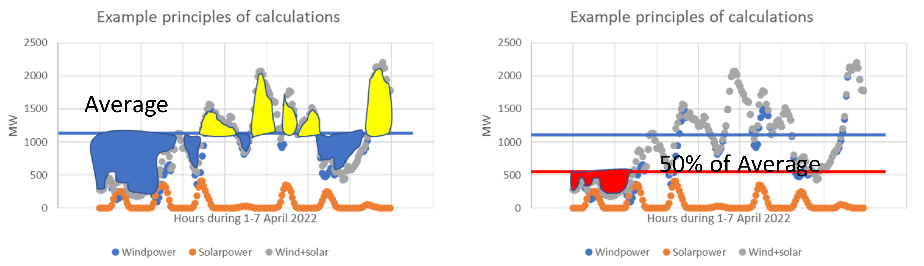
In Figure 7, periods and accumulated energy (kWh) from solar plus wind power below and above average power are shown for January, April, July, and October 2022. Above average corresponds to battery charging, whereas below average corresponds to discharging batteries. The average power production for 2022 was 1070 MWh/h in SE-3. Above the zero-axis is surplus power for charging batteries, whereas below the axis is deficiency, when battery storage was discharged to maintain a constant power production.

In Table 1, the time from when the production passed the average production value per month and the accumulated energy in MWh during the period is presented. Negative values below the average are in white and positive values above the average are marked in yellow.

In July, solar power compensated for varying winds. In July, the periods below and above average were generally more frequent and shorter than during January in particular. The longest period with low wind was 76 h once in July, with the second longest period lasting 42 h. For the other months, there were up to 130 h of low wind in January, 114 h in April, and 109 h in October. However, the deficiency was mostly below 60 h, or 2.5 days. The deficiency was then around 35 GWh for SE-3 in January, 28 GWh in April, and 76 GWh in October, but only 20 GWh in July for the second longest time periods. This was for all periods below and above average power production. The figures vary between years, but not much, as both wind and, to some extent, cloudiness were relatively random throughout the year. The difference between seasons was similar, especially with respect to solar-power production.

In Figure 8, the same data are presented for periods below half of the average power production during 2022.

As shown in Figure 8, the longest period below average in 2022 during January, April, July, and October lasted 130 h and 100,000 MWh of energy were accumulated. For half of the average, the corresponding longest period lasted 55 h and the maximum accumulated energy was 60,000 MWh.

The question then arises of what the case would be if there was five times as much wind-power production and 15 times as much solar-power production, with same distribution as for 2022. The figures are based on predictions for scenarios generated by the Swedish power board [18]. In Figure 9, the result of that calculation is shown for accumulated energy when production is below half of the annual average production of wind plus solar power.

The number of hours was generally the same as for the much lower production in the 2022 case, but the absolute energy was 90,000 MWh compared to 60,000 MWh in the original case for 2022.

There were significant periods with high wind production but also periods with almost zero production.

The wind-power production varied quite rapidly, as shown in Figure 10 (in SE-3). Production changed from almost zero to 2000 MWh/h for SE-3 in less than 12 h.

As a comparison, hydropower production in SE-3 during the same period of 16–25 May 2021 is shown in Figure 11. As can be seen, it slowly moved from 1200 to 1500 MW, which is a very different pattern compared to that of wind-power production.

Looking at only two days, 24–25 May 2021, a very strong variation in wind-power production throughout the day for SE-3 can be seen (Figure 12).

With an average of approximately 1000 MW over two days in SE-3 (actual average value was 1070 MW 2022), it would have been beneficial to store energy in, e.g., batteries; use it on 24 May; and then recharge the batteries on 25 May. In this case, the storage capacity should have been 24 h * 1000 MW = 24,000 MWh, or 24 GWh. A shift of 500 MW from 12 p.m.–9 p.m. (9 h) would mean reducing the peak deficiency by approximately half, or 12 GWh. Looking at the solar power produced in SE-3 during the period of 16–25 May 2021, it appeared as shown in Figure 13.

The main balancing resource was hydropower. In Figure 14, the production in MW during one year from 1 June 2020 to 1 June 2021 is shown for SE-3.

Solar plus wind power followed hydropower, whereas other thermal power was either reduced or kept at a low level. This means that the balancing resources were not utilized. It can also be seen that when solar plus wind power was reduced, consumption was reduced. It should be noted that the price went up during these time periods, which shows that a shifting load can be as efficient as using storage to compensate for reduced power (see Table 1 and the discussion related to this).

In Figure 15, hydropower production for Sweden as a whole and for SE-3 in 2022 is shown. The production in SE-3 was much lower than in Sweden as a whole, which makes it important to be able to import from northern Sweden. Without nuclear power in SE-3, it would be a problem to supply what is needed in the region.

The production in SE-3 was only 10–15% of the total hydropower production in Sweden (approximately 1000 MW compared to 8000 MW on average). It is more difficult to store larger volumes in southern Sweden than in the north, as well.

On the other hand, there was much more other thermal power in SE-3 than in the other regions. This was mostly CHP production. The installed capacity was approximately 5000 MW, whereas only about 900 MW were used in the summertime in all of Sweden, and normally less than 2000 MW were used even in midwinter, when the production was at its maximum. In Figure 16, the monthly production and consumption for the first half of 2022 are presented.

The total production this year was 11.1 TWh_el hydropower for SE-3 and 73.6 TWh_el for all of Sweden (see Figure 15). There was lower production from June to October, but it increased during the winter until March. Generally, the production relates to how much rain falls, and in the spring it relates to how much snow melts. There is normally a possibility to vary power production within a day or a few days in the SE-3 region, but not long term in this densely populated region without the possibility of storing larger volumes of water. Still, this time horizon is normally acceptable to compensate for significant wind-power fluctuations, but with a limited amount of MWh. This capacity varies with the present situation, as weather conditions vary continuously. Whereas wind power is affected by the wind, hydropower production is affected by the rain. Figure 17 shows solar-power production during a period in May. As can be seen, there was a variation between day and night, as well as a significant variation from one day to the next depending on cloudiness. The solar-power pattern was generally possible to predict throughout the year and day by day, but varied throughout this span of time due to varying cloudiness. Still, the intensity and hours per day were much higher during summer than during winter (see Figure 16).

Wind power varied more irregularly, although normally there was more wind during spring and autumn.

Low wind with less than 500 MW production was quite frequent throughout the year for periods of up to approximately 48 h. Longer periods of 100 h or more below 500 MW occurred only five times from June 2020 to May 2021 (Figure 18).

PV production can generally be calculated as a function of the day of the year and the kWh/h.m² for a certain site. This value is multiplied by a factor 0.5–1, where 1 means that there are no clouds and 0.5 means that it is very cloudy. Hourly values were summarized per month. For a region like SE-3, these values were multiplied by the number of m² PV cells in the area. For wind power, the total wind-power production was multiplied by the dimensional wind. This was then multiplied by the predicted actual wind speed divided by the nominal wind speed for an average plant. This was multiplied by the number of hours to obtain the kWh produced during a certain period. Hydropower production was predicted from the average production for each month based on the season and adjusted for rain in relation to the average amount of rain for the season per month. For CHP and nuclear plants, total flexibility was assumed up to the maximum production.

Wind-power production was multiplied by different probabilities to obtain the average wind in the region for the next 24 h, 48 h, 120 h, and 240 h. For solar power, cloudiness values were predicted from weather forecasts for the same time periods. From these estimations, the production from wind plus solar power was calculated for an average case. The accuracy of the prediction relies on how correct the weather forecasts are. The tool can be used to estimate demand for storage capacity and demand for load shift.

3.6. Future Trends in Wind-Power Production

In Figure 18, a statistical analysis of the wind variations in SE-3 for June 2021–June 2022 was carried out. This shows how long the drop below 535 MW lasted in relation to the average 1070 MW.

On approximately 10 occasions it lasted longer than 48 h: Five times it lasted four days or longer and once it lasted more than 10 days. Wind power is expected to grow from 33 TWh/y in 2022 to 120 TWh/y by the year 2040, according to Swedenergy [27]. The capacity factor in 2021 was 0.28, but for new land-based plants it was 0.37. This is predicted to be 0.4 by 2025 due to higher towers. For sea-based wind power it is predicted to be approximately 0.5, which is already the case for new plants at Dogger Bank in the UK. The Swedish Energy Agency [28] expects 5–10% of all power produced in SE-3 to be from the sun and that about 10–20 MW solar power will be in operation by 2040.

3.7. Effect of Price on Power Consumption

At Sala-Heby Energy (SHEAB), a variable cost of power during high-use hours vs. low-demand hours has been implemented for more than 10 years. An electricity reduction of 20–25% was achieved during the daytime when power demand was high, but a new peak was seen just after the low rate started at 7 p.m. In Sweden, a strong reduction in electricity consumption was seen due to high electricity prices during 2022. The electricity consumption decreased by 5% in all of Sweden during January–October 2022 compared to 2021 [29]. In SE-4 it was 20% lower. Electricity prices were as shown in Table 2—twice as high in 2022 compared to 2021 in SE-3 and SE4, but less than 50% higher in SE-1 and SE-2 in northern Sweden. This gives an indication of the effect electricity prices can have on consumption.

3.8. Storage Size

Concerning battery storage, power companies now invest in quite large battery storage to compete with the frequency market. Uppsala has invested in 5 MW, 20 MWh storage [30]. Other cities have planned larger batteries with a 20+ MW capacity, which can be used for both voltage and frequency control (oral communication with Eskilstuna Strängnäs Energy and Environment and Stockholm Exergi).

Table 2. Nordpool historical spot prices in SEK/kWh in 2018–2022 [31].

Year	SE1	SE2	SE3	SE4
2022	0.634	0.664	1.379	1.62
2021	0.432	0.433	0.67	0.817
2020	0.15	0.15	0.221	0.269
2019	0.401	0.401	0.406	0.421
2018	0.454	0.454	0.458	0.476

Table 2. Nordpool historical spot prices in SEK/kWh in 2018–2022 [31].

Year	SE1	SE2	SE3	SE4
2022	0.634	0.664	1.379	1.62
2021	0.432	0.433	0.67	0.817
2020	0.15	0.15	0.221	0.269
2019	0.401	0.401	0.406	0.421
2018	0.454	0.454	0.458	0.476

Figure 18. Time periods with less than 535 MW wind-power production in SE-3 compared to the average of 1070 MW from 1 June 2020 to 31 May 2021 [31].

Figure 18. Time periods with less than 535 MW wind-power production in SE-3 compared to the average of 1070 MW from 1 June 2020 to 31 May 2021 [31].

From the previous calculations, it was determined that the appropriate size of battery storage for SE-3 is not self-evident. For the situation in 2022, the average production from wind plus solar power was 1070 MW, and half of that is 535 MW. For a scenario in 2045 with five times more wind and 15 times more solar production, the average production for wind plus solar power would be 6137 MW, and half of that is 3069 MW. For the first case, the accumulated deficiency, which is the area below the line halfway between average and zero production, for the periods of January, April, July, and October was the longest at 55 h and 60 GWh. For 2045, the storage demand for the longest period below half of the average would be 90 GWh and would have a longest deficiency period of 63 h. It would be reasonable to determine the amount below half of the average for a battery and/or H₂/FC. The rest should be balanced with hydropower, other thermal power, and reduced consumption during low-wind periods through different types of financial agreements with industry and increased prices in general, which proved to be efficient during 2022.

The alternatives with 12 or 24 GWh storage capacity for the 2022 case and 6.4 or 37 GWh predicted for 2045 for periods below the 50% average yielded values proportional to the calculations for 60 and 90 GWh for periods below average. At least for today’s case, 12 or 24 GWh may be more realistic, but for the 2045 case the alternative with 37–90 GWh would probably be more realistic, as the proportion of wind plus solar power would then be much larger, whereas hydropower and CHP would probably be the same as today. On the other hand, much of the new demand will be for industries that may solve many of the balancing problems internally with large amounts of H₂ storage.

Technical data for H₂ production, NH₃ production, and battery storage are provided in, e.g., [32,33].

The storage volume and weight are shown in

Table 3. kWh battery capacity per ton and m³, both with and without losses.

		Excluding Losses		Including Losses
		kWh/ton	kWh/m3	kWh/ton	kWh/m3
Batteries
1st life		200	300	180	270
2nd life (70%)		140	210	126	189
H2/FC 700 bar		33,600	2478	19,837	1463
NH3		5910	4300	2656	1932

per m³ and ton, respectively. In

Table 4. Weight and volume for 60 GWh (2022 case) and 90 GWh (2045 scenario) storage capacities.

	60 GWh Includ Losses		90 GWh Includ Losses
	ton	m3	ton	m3
Batteries
1st life	333,333	222,222	500,000	333,333
2nd life (70%)	476,190	317,460	714,286	476,190
H2/FC 700 bar	3025	41,012	4537	61,517
NH3	22,593	31,052	33,889	46,578

, the total weight and volume for the case with the longest period below half of the distance between the average annual production and zero production is presented: 60 GWh (2022 case) and 90 GWh (2045 scenario). In

Table 5. Weight and volume for 6.4 GWh (2022 case) and 37 GWh (2045 scenario) storage capacities.

50% of Aver*12 h	6.42	GWh	37	GWh
	ton	m3	ton	m3
Batteries
1st life	35,667	23,704	205,556	137,037
2nd life (70%)	509,952	33,862	293,651	195,767
H2/FC 700 bar	323	4375	1865	25,290
NH3	2410	3312	13,932	19,149

, the case with 50% of the average power over the year for 12 h is presented: 6.4 GWh (2022 case) and 37 GWh (2045 scenario).

For electrolyzers, there may be 82% efficiency in the future and 80% for fuel cells. To compress the gas to 700 bars would consume at least 10% of the heating value of the hydrogen, which would be converted to heat. This would yield a system efficiency of 0.82*0.8*0.9 = 58%. However, today it is closer to 0.6*0.6*0.9 = 32% system efficiency, at least for the next few years. For the combination of batteries with EVs there would more likely be 0.8*0.8 = 64% to potentially 0.9*0.9 = 81% system efficiency, with the potential to become even higher.

To store energy as NH₃, first H₂ and N₂ must react to form NH₃. The conversion efficiency for H₂ to NH₃ is about 61–68.5%. This means that with an 82% electrolyzer efficiency and an 80% fuel-cell efficiency the total would be, assuming 68.5% H₂-to-NH₃ efficiency, a system efficiency = 68.5*82*80 = 45%. For batteries we calculated 90% and for H₂/FC 82*80% = 65.6%.

For the case with the longest period below half of the distance between the average annual production and zero production we calculated the size of storage to be 60 GWh for 2022 and 90 GWh for the predicted 2045 scenario.

The size with respect to storage in weight in tons and volume in m³ is the total. How much local storage there should be is not clear—either a few large storage facilities connected to some large production sites, a large number of local storage facilities connected to local production, or a combination of the two. The latter is the most probable. Table 5 shows the case with short-term storage over 12 h but with significant power, half of the power based on the average, and half of the average for the 2022 and 2045 cases.

For the first case the difference between the 2022 case and the 2045 scenario was quite small but was significant for the 12 h storage.

As can be seen, H₂ takes up less space, but to build huge storage facilities requires digging out deep cylinders in the rock to provide support to the steel vessel. Concrete is then filled in between the cylinder and the rock wall. This is currently being demonstrated in Luleå with the Hybrit project [34]. For batteries, State Grid in China together with Rongke Power just built a 100 MW/400 MWh vanadium sulphate/vanadiumoxidesulphate redox flow. This shows the possibility of building large-scale batteries [35]. This is a USD 266 M investment. Pump storage had an installed capacity of 160 GW and 8500 GWh in 2020 globally. This accounted for 90% of global electricity storage [36]. As a comparison, the battery factory in Skellefteå, Sweden, built by NorthVolt, will have a capacity of 60 GWh/year when full capacity is reached within a few years [37].

Concerning costs, NREL [38] made some estimates for lithium-ion batteries with 4 h storage capacity, as shown in

Table 6. Estimated cost for lithium-ion batteries in million USD for different sizes in GWh [38].

GWh	6.4	37	60	90
M$	960	5550	9000	13,500

.

The figures are high, but in proportion to other infrastructure investments they are reasonable.

As is shown, there are several alternatives that will have advantages and disadvantages. The most probable scenario is a combination of all type of solutions. For batteries, it can be noted that a capacity of 5 million EVs with 100 kWh/vehicle would be 500 GWh. Today, there are 5 million personal cars in Sweden, which could be predicted to be all EVs in some capacity in the future, and 100 kWh/car should be a realistic size in the future. This suggests some proportions of the size for grid support with charging infrastructure and power supply.

3.9. Balancing with CHP

Concerning CHP (combined heat and power) with biomass or waste as the fuel, most power production is carried out during the winter, when there is a high heat demand. It is possible to produce more electric power by condensing steam with sea water or air if the electricity demand and price are high. For Sweden, there was an estimate made by Svebio [39] that about 35 TWh/y could be produced from existing plants compared to 12 TWh/y produced today, due to financial conditions.

In Figure 16, it can be seen that the relative-capacity factor for hydropower and nuclear power was highest from January to March. For solar power and PV, the maximum was in May–July, whereas wind power showed the opposite trend, as it was highest during January–March and lower during summer. For thermal power other than nuclear, mostly CHP, high production was evident during winter in January–April, but it dropped significantly during the summer, when the heat demand was lower.

Table 7. Electricity production and consumption in GWh/month in Sweden in 2022 [11,12].

	Wind	Hydro	Nuclear	OthThermal	PV	TotProduc	ToConsum
	GWh	GWh	GWh	GWh	GWh	GWh	GWh
Jan.	4225	6176	4963	1027	7	16,398	−13,735
Feb.	3636	6009	4349	831	21	14,846	−12,385
Mar.	3319	5990	5131	946	93	15,479	−12,291
Apr.	2237	5703	4487	784	127	13,338	−10,932
May	2770	5175	3762	587	163	12,457	−9707
Jun.	1854	5382	3677	343	182	11,438	−8768
Jul.	2250	5649	4096	276	185	12,456	−8418
						96,412	−76,236

shows the actual figures in GWh/month for January–July 2022 with respect to power production and consumption.

The production and consumption proportions were similar for SE-3, despite all nuclear being produced in SE-3 but only 15% of hydropower. Hydropower outside of SE-3 was used to balance demand in SE-3. In Table 3, the installed capacity and the maximum power for each month during the same time is shown. In

Table 8. Relative-capacity factors C_p,r for Sweden during spring 2022.

	GWhmax	Jan.	Feb.	Mar.	Apr.	May	Jun.	Jul.
Wind	4225	1	0.86	0.79	0.53	0.66	0.44	0.53
Hydro	6176	1	0.97	0.97	0.92	0.84	0.87	0.91
Nuclear	5131	0.97	0.85	1.00	0.87	0.73	0.72	0.80
Thermal	1027	1.00	0.81	0.92	0.76	0.57	0.33	0.27
PV	185	0.04	0.11	0.50	0.69	0.88	0.98	1.00

, the relative-capacity factor C_p,r is shown to vary for the different technologies.

The relative-capacity factor C_p,r is calculated as the ratio of the maximum power during one month divided by the power produced for each month. For wind and PV the C_p,r is based on the weather, whereas hydropower can be controlled to some extent. Nuclear power normally operates at the maximum possible capacity continuously, and thus reduced C_p,r is due to technical problems. For thermal, mostly CHP, a low C_p,r is seen during warm periods.

What is of special interest is that the maximum power for thermal power other than nuclear was approximately four times higher than what was produced during spring and summer. This demonstrates great potential to use bio-CHP to balance the lower wind-power production seen during spring and summer. In addition, new PV-cell systems on the roofs of buildings will be expanded and will provide another opportunity to complement wind power during summer. In absolute figures, CHP using biomass and waste could double the production compared to today during winter if heat can be utilized for other applications. Existing CHP plants could be complemented with pyrolysis to produce bio-oil and gasification for the production of H₂ and CH₄. This would provide the opportunity to increase wind power significantly and still maintain balancing power, as the focus can be on electric-power production during the time periods of a lack of power from wind. In

Table 9. Installed max power (MW) and used max power (MW) during January–July 2022 in Sweden [11,12].

2022	Wind	Hydro	Nuclear	Thermal	PV
	MW	MW	MW	MW	MW
Installed	10,017	16,334	6871	4399	1090
Jan.	10,067	12,143	6940	1959	215
Feb.	9863	12,393	6943	1824	465
Mar.	9254	12,241	6944	1908	701
Apr.	9428	11,665	6925	14,983	907
May	9146	9649	5717	1407	994
Jun.	6447	9935	5702	1013	1060
Jul.	6590	10,522	6540	891	1054

, the installed and max capacity per energy type and month in January–July 2022 are shown.

To store 500 MW for 48 h a capacity of 24 GWh is needed and for 12 h a capacity of 6 GWh is needed for the SE-3 region in today’s conditions (2022). Looking at the demand for all of Sweden, the corresponding figure would be three times as high, or about 72 GWh. Going from 33 TWh/y in wind power as today to about 90–120 TWh/y within 20 years as discussed, the demand for storage capacity may increase to 80–100 GWh for 48 h. On the other hand, if hydrogen is produced for industrial use, at least half of this may be covered by H₂ storage if conversion efficiencies are increased and costs decreased for H₂ storage. The CHP plants could yield a maximum of 4399 MW * 48 h = 211 GWh for 48 h. If some of that potential is used together with batteries, a very promising balancing potential would be achieved.

Looking at Figure 18, it can be seen that 48 h storage was enough in most cases over the year. However, on one occasion the low wind lasted for 250 h. This would be difficult to cover completely with stores of batteries or H₂. From an economic perspective it would be reasonable to restrict the power demand during this time by increasing the price or by shutting down some demand during shorter time periods. However, production by CHP could cover much of that demand, especially if it happens during the winter season. There is also a potential to increase hydropower production during at least the winter season by some 1000 MW * 48 h = 48 GWh for a couple of days, and if it is rainy perhaps for all 10 days. However, during dry weather conditions this may be difficult. Where the demand is in relation to where the production is must also be considered. CHP plants are well distributed in SE3, where there is high heat demand from many people, whereas hydropower is mostly in the northern part of Sweden. By distributing battery storage close to where the potentially high demand is, it would be easier to balance without having to expand the grid capacity significantly.

Another aspect is the cost for different storage alternatives. It is not obvious what the cost would be for pump storage, as it would vary a lot depending on the situation. The company Mine Power is looking into using old mines for pump power with high potential in the SE-3 region. As for batteries, the average cost for new battery packs was in the range of USD 150/kWh in 2022, according to Blomberg News [40]. The cost for just the cells was at average of USD 115/kWh. An interesting alternative is to use second-life batteries. It is not easy to know exactly where the price for these will end up. If it is assumed that 80% of the original capacity is still in the battery after its first life, potentiallya bout 10–30% could be used before the end of its life. This will vary with the battery chemistry. NMC batteries usually have a relatively flat degradation rate for a certain number of cycles but then start to drop rapidly. For LFP batteries, the degradation rate is slower but lasts more cycles; however, they are much heavier in weight per kWh storage capacity. There is a demand to determine the state of health (SoH), and from this the remaining useful life (RUL) for second-life applications. If this can be determined in a reliable way and the batteries can be used without reconfiguration, the price should be significantly lower for each stored kWh in a second-life battery than for a first-life battery. How much that would be is a guess, but it would perhaps be in the range of half of that for first life. However, the cost of new batteries has been decreasing, although it flattened out during 2022 [40]. The cost for battery materials is increasing due to short supply, but the interest in recycling batteries for new first-life batteries is high, and most batteries are expected to end up this way. If new batteries are too inexpensive, it will be of less interest to use them in a second-life application. There will also be additional costs for the installation and operation of battery packs.

4. Discussion—Balancing Demand/Supply Using Batteries and Varying Electricity Price

A load shift can be a good alternative to balance swings in wind intensity and thereby swings in electricity production, aside from balancing with additional production from other sources such as hydropower and CHP. Today, there are almost no incentives or only small ones for most companies and residential users to shift load—or there was not until 2022, when the increased fossil-fuel prices caused electricity prices 10–20 times higher during periods with low wind-power production in Europe. If this were a more long-term situation, it could give incentives for new investments. Exceptions are some energy-intensive industries where agreements between suppliers and customers can often handle load shift or even stop machines temporarily, or increasing additional power production at a plant.

The variation in power demand over a year in Sweden was between 9000 and 24,000 MW throughout the seasons during 2022, with peak power during shorter periods of hours or a few days, with variations of approximately ± 2000 MW. For SE-3, the power consumption was 62.5–63.5% of that for all of Sweden during 2021–2022. For SE-3, the corresponding figure is ± 1000–1200 MW within a few days. A load shift in the range of 1000 MW and 500–600 MW for 6–9 h was usually seen to reduce the peak loads by up to 70%. These rough figures were used to make it possible to reduce the battery storage to half the original size estimated, yielding a demand for 12 GWh and 40 GWh to balance SE-3 and Sweden, respectively, if hydropower, CHP, or H₂ is utilized to balance storage. If the worst case from 2022 is considered, the demand may be significantly higher, as shown in Table 1, at about 60 GWh for just SE-3.

4.1. Discussion of Storage Costs

For a residential user (family) without electric heating the annual consumption may be 2500–4500 kWh/y. With an electricity cost of USD 0.05/kWh the total cost would be USD 125–225/y. With this come taxes and fixed costs of around USD 250–450/y. As can be seen, the actual electricity price plays a minor part. If fixed costs and taxes are also varied depending on the situation, the total cost could be USD 375–675/y. This can then vary over time in the range of USD 100–200/y for the total cost. If electric heating is added, it could mean another 10,000–20,000 kWh/y and USD 1500–3000/y. At that point, a varied price would start to become an issue for most people. It should be noted that about 16–20 TWh/y are used for electric heating of buildings in Sweden. If a 20% price increase is assumed, it would mean (1875–3675) * 20% = USD 375–735/y. By cutting these costly peaks with a battery the potential annual cost for the battery would require a maximum of USD 375–735/y for a house with electric heating and only USD 20–40/y for an apartment without electric heating to be profitable. With a 40% higher electricity price instead, all figures would generally be doubled. In 2022, prices were about ten times higher for several months. Spread throughout a year, the high peak price yields a lower effect, but would at least be higher than the 40% increase and likely closer to a 100% increase. By shifting the heat load and using a battery when electricity prices are high, it may be realistic to consider a local battery pack in the future. With second-life batteries, the capital cost for these could be low. For a two-day period with a big difference in wind-power capacity it should be possible to shift the load demand significantly. As the power demand in Sweden is estimated to increase to 85 TWh/y and 45–50 TWh/y, nuclear power will be shut down within 20–25 years and about 130 TWh/y new capacity is needed [17]. All nuclear power is in the SE-3 region, but a significant share of the new power demand is in the northern part of Sweden for industrial use. With a new government since 2022, interest in developing new nuclear power has increased and may replace the existing nuclear-power plants when the technical lifetime is reached around 2040–2045. However, there will be a shortage of some 70–90 TWh/y that need to be added just in the SE-3 region. Most of this will be from wind power, and thus the variation in wind-power production will be significantly larger than today, with 33 TWh wind power/y (2022) and 45–50 TWh/y nuclear power. This means that thermal power (mostly CHP) and batteries may be needed to a much higher extent than anticipated today to balance four to five times more varying wind power. With higher wind-power towers this could be reduced to perhaps half, as wind varies much less at higher heights and offshore. Luthander et al. [41] studied balancing between load and PV-cell production for residential areas. This is of interest, but would probably not yield a significant amount compared to the demand. One alternative that will be of high interest is to produce hydrogen from wind power and possibly also PV power. The hydrogen can be stored in large tanks. It can be produced when there is a surplus of wind and be used when there is a shortage of power. Especially for industrial processes such as steel manufacturing and oil refining, large amounts of hydrogen will be needed. By having hydrogen storage, both the demand in these industries and the capacity to use it in applications with vehicles with fuel cells or hydrogen engines can be achieved. This will compete with batteries. However, from a system perspective, batteries have higher efficiency. Therefore, from a system perspective batteries are good but demand many special metals and elements in the manufacturing. Both alternatives will be achieved in parallel. Other aspects will guide where one technology or the other is utilized. Still, second-life batteries may have an important role, as they increase the total life cycle of batteries. If the primary life for EV batteries is assumed to be 80% of the initial capacity, the same batteries down to about 50–60% of the initial capacity can be used for stationary applications before the batteries are sent for recycling. This makes the possibility of large storage capacities feasible in the future, but the cost calculations are still uncertain. Malardalen University is running a project called RECREATE [42] with a focus on the second life of batteries. The project includes vehicle manufacturers such as Volvo (trucks, construction equipment, buses), Epiroc (mining equipment), and Alstom (trains), as well as users of second-life batteries, including energy companies such as Malarenergi and ESEM (Eskilstuna Strägnäs Energy and Environment). We have been investigating different business models and how to design battery packs directly for easy use as second-life batteries without a lot of remanufacturing. The number of cycles before the end of first life is usually an estimate in an initial contract. The actual use of the batteries, such as how deep the cycles are and thereby how fast the deterioration is, remains to be measured. From this and based on separate measurements after the first life of battery packs, the remaining useful life (RUL) is estimated. This makes it possible to create business agreements for second-life operations. Generally, the price is about USD 150–250/kWh for the first life for lithium-ion batteries, and we believe it could be reasonable to expect half of this for second-life batteries. On the other hand, a second-life battery will have a capacity of only 70–80% of a first-life battery. Therefore, there will be negotiations regarding pricing. Finally, the batteries will be recycled to a battery-scrap company. Northvolt Revolt is a company driving this and plans to use up to 50% of the raw material for new batteries from recycled batteries withing about 10 years. Primarily NMC Li-ion batteries but also LFP and NiMH batteries are included in the study. For the time being, lead batteries are not included.

The Swedish power production in 2020 with different production means is shown in

Table 10. Installed power capacity and electricity production for Sweden in 2020. Other thermal power production is the sum of condensing, CHP, GT (gas turbine), and industrial backpressure [11,12].

Production 2020	MW	TWh/y
Hydro	16,335	71.2
Nuclear	6871	47.3
Condensing	905	1.8
GasTurbine	1583
CHP	2879	10.9
Ind BackPressure	1520
Wind	10,017	27.6
PV	1100
Total	41,210	158.8
Est prod Capacity	24,900
10 y winter demand	27,800
Therm oth than nucl	6887

.

It can be seen here that the highest installed capacity was in hydropower, with wind power as number two. Nuclear power and thermal power other than nuclear had roughly the same installed capacity. However, other thermal power (sum of condensing, CHP, gas turbine, and industrial backpressure) only produced 12.7 TWh in 2020 compared to 47.3 TWh for nuclear, as the installed capacity was not used that many hours per year for electricity production due to economic conditions. There is a significant potential to increase this if electricity prices goes up, and it can cover a significant power-balance effect, in addition to batteries, hydropower, and potentially hydrogen. If CHP plants are operated not only when the weather demands it, a total of about 35 TWh electricity could be produced per year according to [39], as mentioned earlier.

4.2. International Perspective

Eurostat is keeping control over the energy situation in the EU [43]. Wind, hydro, and solar were used to produce 32.8% of the net electricity generated in the EU in 2021. Total net electricity generation in the EU was 2785 TWh in 2021, similar to 2020 (−0.1%).

The EU has several different regional markets that are being interconnected successively.

There are discussions about long-distance interconnections to overcome limitations with renewables. If the whole world is interconnected there will always be sunshine somewhere, and wind and rain will provide wind power and hydropower globally instead of only locally. In [44], an investigation was conducted on an interconnection between China and the EU. Four scenarios with 100% renewable energy were conducted to identify the best option for achieving an hourly power balance with or without storage. The electricity interconnection between CN (China) and the EU decreased annual additional costs by more than 30% compared to the absence of the interconnection, which demonstrates the necessity and benefits of a CN–EU electricity interconnection.

In [45], an analysis of the EU electric-power market was conducted quarterly. There are seven regional wholesale markets in the EU: Northern Europe, Central–Western Europe, the British Isles, the Apennine Peninsula, the Iberian Peninsula, Central–Eastern Europe, and Southeastern Europe. The goal is to integrate these regions in the longterm. Today, Nordpool for Northern Europe is a well-functioning market and is working with several of the closest markets, such as the British Isles and Central–Western Europe.

5. Conclusions

The conclusion from this analysis is that in Sweden, a storage capacity such as, e.g., a battery with a capacity of roughly 6–60 GWh would be needed for the SE-3 region and three times as much for all of Sweden to cover the biggest difference between wind-power production vs. demand today if no other means were used. If shifting load is utilized with the incentive of higher electricity prices during shortage periods and complementing it with hydropower and thermal power other than nuclear power, a significantly smaller battery would make sense and be economical. For a battery with a capacity of 6.4 GWh, for the 2022 case a battery of the size of 37 GWh would be needed in a future 2045 scenario with five times more wind power and 15 times more solar power. This would cover 50% of the power between the annual average and zero production. For a case in which the longest period was below the annual average, the corresponding values are 60 GWh for the 2022 case and 90 GWh for the 2045 scenario. The cost would be USD 150 M per GWh according to NREL, who based the costs on a lithium-ion battery with a 4 h storage capacity [38].

If there is low wind, the nuclear reactors stop, or similar occurrences take place and last for longer time periods, such as days or even week or months, the first action is to increase the price. This proved to reduce power demand by 5–20% depending on price during 2022 in Sweden. Secondly, industries are asked to reduce power demand. By doing so, they receive economic compensation (if agreed on in advance). Thirdly, SVK (the Swedish power board, controlling the power balance) has agreements with several old power plants to start these on request, although using fossil fuels, and thereby compensate for other power shortages. This needs to be turned into long-term contracts and not only be signed for a year or two in order to stabilize the power system.

The route with hydrogen production and storage is an alternative to batteries and will surely be a parallel technology, especially as several industrial processes will use hydrogen in their processes. Therefore, it makes sense to utilize hydrogen for other purposes as well, e.g., in transportation. Truck manufacturers such as Volvo, Tracton (Volkswagen Truck, Scania, and MAN), and Daimler are looking into the use of hydrogen with fuel cells for long-distance transport with trucks and buses. However, in the long term, much more electricity will be needed to replace fossil fuels in primarily the steel industry and for vehicles (85–110 TWh/y), as well as to compensate for when 45–50 TWh/y nuclear power is phased out. This will be covered mostly by wind. However, by then the variation due to varying wind speeds could be four to five times higher than today, and both CHP and batteries will be needed much more. Second-life batteries then make a lot of sense to use to extend the battery life cycle. It makes a lot of sense to utilize batteries in vehicles as well as second-life batteries in households or for other stationary applications at the local level to make the system robust. With higher wind-power towers, however, the capacity factor can be significantly higher than it is today (50% or higher), and the variation in power production from wind may then be reduced by up to 50% compared to today, and the needed storage capacity may be lower as well.