Online Prediction of Electric Vehicle Battery Failure Using LSTM Network

Abstract

The electric vehicle industry is developing rapidly as part of the global energy structure transformation, which has increased the importance of overcoming power battery safety issues. In this paper, first, we study the relationship between different types of vehicle faults and battery data based on the actual vehicle operation data in the big data supervisory platform of new energy vehicles. Second, we propose a method to realize the online prediction of electric vehicle battery faults, based on a Long Short-Term Memory (LSTM). Third, we carry out prediction research for two kinds of faults: low State of Charge (SOC) alarm and insulation alarm. Last, we show via experimental results that the model based on the LSTM network can effectively predict battery faults with an accuracy of more than 85%. Through this research, it is possible to complete online pre-processing of vehicle operation data and fault prediction of power batteries, improve vehicle monitoring capabilities and ensure the safety of electric vehicle use.

1. Introduction

In order to alleviate the conflict between the ecological environment and fossil energy, energy transition is of great significance to all countries in the world. China has responded quickly to this challenge and accelerated the layout of the electric industry and technology research and development. In the transportation industry, the electric vehicle industry has been ushering in opportunities for rapid development. Electric vehicles have also gradually been adopted by thousands of households. According to statistics, China’s new energy vehicle production has been the highest for eight consecutive years. In 2022, the production and sales of new energy vehicles reached 7.058 million and 6.887 million, respectively, which represented an increase of 96.9% and 93.4%, respectively, compared with the previous year. The market share reached 25.6%, which was 12.1% points higher than that in the previous year.

It is expected that China’s new energy vehicles will continue to maintain rapid growth momentum in 2023, and the annual sales are expected to exceed 9 million vehicles in total, exhibiting an increase of 35% year-on-year [1]. With the growing sales, the safety of electric vehicles has become a topic of concern, and the number of reported electric vehicle fires has increased every year. According to incomplete statistics on the Internet, the number of spontaneous combustions reached 70 cases from January to November 2022, and it was found, using analysis, that 90% of the accidents were caused by power batteries [2]. Therefore, it is significant to study how to accurately predict and warn about failures in advance using historical vehicle data.

After Long Short-Term Memory (LSTM) networks were proposed and improved, they have been used in various fields and have facilitated industrial development. Hochreater and Schmidhuber proposed LSTM in 1997, which could effectively solve the gradient explosion and gradient disappearance problems faced by the Recurrent Neural Network (RNN) during training [3]. In 2001, Felix G. [4] further improved the LSTM network structure by adding a forget gate and a peephole. After the publication of the aforementioned papers, researchers started to apply LSTM networks to their own research areas. The authors in [5,6,7] showed that LSTM was first applied in the fields of text recognition, machine translation and information retrieval. Graves et al. used LSTM for handwritten digit recognition.

Sutskever et al. proposed a method to build a machine translation framework using two multilayer LSTM networks, where one network learnt the characteristics in the source language and then used them and the other network to complete the translation in the goal language. Palangi et al. used LSTM to obtain characteristic vectors of large text or complete articles and then maximized the similarity between the characteristic vectors of the information search and document search to complete the information retrieval. In [8,9,10], the authors introduced the applicability of LSTM networks for the graphical conversion task. They treated the graphical conversion task as a special image to text translation problem, in which the input part uses the Convolutional Neural Networks (CNN) to extract the characteristics of the image, and the output part uses the LSTM networks to generate the text.

With the development and advancement of technology, LSTM networks are being used in a wide range of fields, such as image recognition, sentiment analysis, health assessment, situation prediction, and so on. Liu et al. [11] introduced a technical approach to recognize weld seams using online CNN–LSTM. The authors used the CNN to extract the main features of molten pool images and transformed them into feature matrices. Subsequently, they used these matrices in LSTM networks to carry out feature fusion and to achieve an implicit mapping of molten pool images to weld defects. The test results also confirmed the superiority of the proposed approach. The authors in [12,13,14] proposed image recognition methods based on LSTM networks to construct caption models, which could effectively achieve image recognition and caption generation. In [15,16,17,18,19], the authors introduced methods for constructing sentiment analysis models using a single LSTM network or by fusing other algorithms. By learning and analyzing input texts, comments in social big data, changes in brain electrical activity and sentiment expression texts, etc., the proposed methods achieved the semantic representation and classification of target emotions.

The authors in [20,21] proposed a health assessment method for heart rate monitoring based on the LSTM network. In this method, the LSTM network was used to continuously monitor and analyze the heart rate collected with wearable devices in order to evaluate physical health condition. Ye et al. [22] and Li et al. [23] proposed LSTMCAE and LSTM–VAE health assessment methods based on LSTM networks, and experimentally validated them on turbofan engines and hydraulic pump equipment, respectively. The experimental results showed the usability of LSTM networks in the field of mechanical equipment health assessment. The authors in [24,25,26] introduced forecasting methods based on LSTM networks in the fields of house prices, stock prices, and traffic flow, etc., while using data samples to verify that the LSTM networks could predict future trends based on historical data.

Thanks to the LSTM network’s ability to predict future trends based on historical time series data, it has been increasingly applied to power battery failure prediction in electric vehicles. Hong et al. [27] proposed a power battery voltage fault prediction method using a combination of LSTM networks and alert or alarm thresholds. The method detected the occurrence of a fault in the battery system by projecting the voltage over multiple steps. Zhang et al. [28] proposed a fault diagnosis and prediction method for lithium-ion batteries based on a Lebesgue Sampling LSTM (LS-LSTM) network. It solved the problem of the high computational and training requirements for fault diagnosis and the prognosis of LSTM networks in the Riemann sampling framework. The authors carried out offline and online validation experiments on battery capacity degradation.

Ding et al. [29] proposed a method of diagnosing connection faults in parallel battery packs from the current distribution. The authors determined the presence of connection faults among the packs by analyzing the residuals between the projected current distribution values of the LSTM network and the theoretical values. Trivedi et al. [30] designed a scheme to predict tire pressure failure, temperature failure and electric vehicle battery failure using the CNN and LSTM models. However, most of the methods proposed in the literature are based on a single parameter for fault prediction and there is a lack of correlation analysis between other battery parameters and faults. Furthermore, these methods are based on the experimental model and fail to consider unpredictable situations that occur during the actual operation of the vehicle.

In summary, LSTM networks have been applied to study battery fault prediction; however, these fault prediction studies are experimental and use offline data; further validation is needed to increase the effectiveness of online real-time prediction of electric vehicle battery faults. Therefore, this paper proposes an online diagnosis and prediction method of an electric vehicle power battery fault based on the LSTM network combined with real-time operating conditions to further improve the application value of fault prediction. The rest of this paper is organized as follows: Section 2 briefly describes the working principle and model building of the LSTM. Section 3 introduces the data pre-processing and fault feature analysis. Section 4 shows the experimental scenario and results analysis, and Section 5 concludes the paper.

2. LSTM Principle Methodology and Model Building

2.1. Introduction of the LSTM Principle

Before understanding the LSTM network, we should first understand the RNN, which is a recurrent neural network with sequence data as the input. It is recursive in the direction of sequence evolution and all nodes (recurrent units) are connected in a chain-like manner. The RNN is widely used in tasks such as language modelling, machine translation and sentiment analysis. Its network structure is schematically shown in Figure 1, and the computational expressions are given in (1) and (2). However, it suffers from a long-term dependency problem because it cannot transport information from an earlier time step to a later time step due to its short-term memory. This means that the RNN may miss important information at the beginning and face the problem of gradient disappearance during backpropagation resulting in the neural network not continuing to learn and failing to make predictions.

The computational expressions are as follows:

$$s_t=f(U\times X_t+W\times s_{t-1})$$

(1)

$$O_t= \mathit{Soft} max(V\times s_t)$$

(2)

where $s_t$ and $s_{t-1}$ represent the memory state at time instants t and t − 1, respectively, f represents the activation function, $X_t$ and $O_t$ represent the input and output parameters, respectively, U, W, V represent the different weights, and Soft max denotes the output layer activation function.

The LSTM network is a temporal RNN that determines the retention and loss of input information by adding special gates to the RNN. It solves the vanishing gradient problem faced by the RNN in backpropagation, which in turn allows the prediction of data information in a time series.

Figure 2 shows the overall structure of the LSTM network, which adds three addition interaction layers to the RNN, mainly three σ (activation functions) and a tanh layer consisting of internal input gates, forget gates, and output gates, thereby controlling the update, storage and loss of information in the network structure. Each gate works as follows:

Assuming that there is a time series of data X ($\mathrm{x}1$,$\mathrm{x}2$, $\mathrm{x}3$, …, $\mathrm{xt}$) and the hidden layer is H ($\mathrm{h}1$, $\mathrm{h}2$, $\mathrm{h}3$, …, $\mathrm{ht}$), the internal calculation process of the network is as follows:

(1)

Forget gate: The inputs $x_t$ and $h_{\mathrm{t}-1}$ are used, and the activation function determines which information is lost and retained in the LSTM memory cell, calculated as follows:

$$f_t=\mathsf{\sigma }(W_f·h_{t-1}+W_f·x_t+b_f),$$

(3)

where $f_t$ denotes the output value of the forget gate at time t after the application of activation function σ. Sigmoid function is used as the activation function that compresses the output value between 0 and 1, $x_t$ denotes the input value at time t, $W_f$ denotes the weight of the forget gate, $h_{t-1}$ denotes the state of the hidden layer at the previous time instant, and $b_f$ denotes the bias of the forget gate.

(2)

Input gate: The information in the memory cell is updated using the following expressions:

$$i_t=\sigma (W_i·h_{t-1}+W_i·x_t+b_i),$$

(4)

$${\tilde{C}}_t=\tanh \left(W_C·h_{t-1}+W_C·x_t+b_C\right),$$

(5)

where $i_t$ denotes the output value of the input gate after the application of the activation function at time instant t, $W_i$ denotes the weight of the input gate, $b_i$ denotes the bias value of the input gate, ${\tilde{C}}_t$ denotes the state of the cell at the current moment, tanh denotes the activation function, $W_C$ denotes the weight of the cell, and $b_C$ denotes the bias of the cell.

Integrating the results of the forget and input gates, the output value of the cell state at time instant t can be calculated as

$$C_t=f_t\times C_{t-1}+i_t\times {\tilde{C}}_t,$$

(6)

where $\times$ denotes the product of two vectors, and $C_{t-1}$ denotes the cell state at the previous time instant.

(3)

Final output gate: The output information is determined using the following expression:

$$o_t=\mathsf{\sigma }(W_o·h_{t-1}+W_o·x_t+b_o),$$

(7)

$$h_t=o_t\times tanh\left(C_t\right),$$

(8)

where $o_t$ denotes the value of the output gate at time instant t after the application of the activation function, $W_o$ denotes the weight of the output gate, $b_o$ denotes the bias of the output gate, and $h_t$ denotes the output value of the model at time instant t, i.e., the predicted value.

2.2. Fault Prediction Model Building

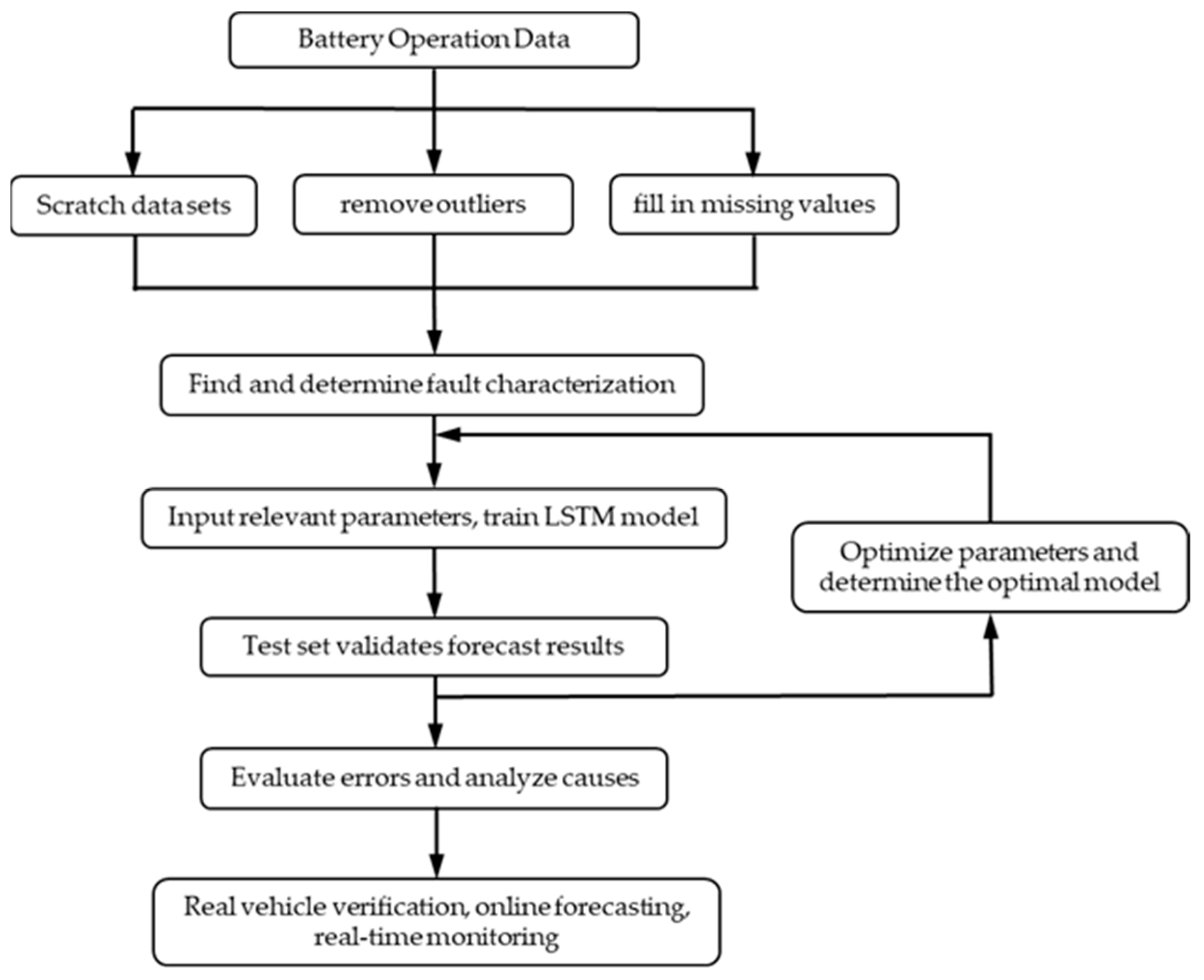
The fault prediction model is based on the working principle of the LSTM network model in Section 2.1. First, the data samples are divided according to the different fault types. Second, the data characteristics are analyzed to find the fault characteristic parameters. Third, the input and output parameters of the model are determined. Last, the model is trained to find the optimum parameters in the prediction model, such as the number of time steps, learning rate, batch size, number of fully connected layers, training times, etc., so as to achieve the best prediction performance. Figure 3 shows the battery failure prediction process.

3. Data Processing and Characterization

3.1. Data Description and Pre-Processing

The vehicle data used in this paper are available from the online database of the Guangzhou new energy intelligent vehicle big data monitoring platform. The operation mode of the vehicle is pure electric mode, and there are two types of vehicles. The data are collected in the period between April to October 2022 at a sampling frequency of 20 Hz during normal vehicle operation (simply recorded as 20 s/time), and a sampling frequency of every 2 Hz in the event of a fault (simply recorded as 2 s/time). The vehicle dataset used in this paper totals 6,568,070 pieces of data, and information on 55 characteristics, including battery operation data, drive motor data, fault codes, etc.

Table 1. Table providing an explanation of the vehicle operation data.

Field Name	Example
Max. alarm level	0	1	…	3
Vehicle speed (km/h)	68.6	101.2	…	0
Vehicle status	1	2	…	1
Mileage (km)	27,326.3	27,341.4	…	27,356
Total voltage (V)	358	355	…	360
Total current (A)	156.4	−9.7	…	−19.1
SOC (%)	78	78	…	5
Insulation resistance (kΩ)	1000	1000	…	11
Max. cell voltage (V)	3.943	4.001	…	3.921
Min. cell voltage (V)	3.926	3.99	…	3.909
Alarm information	0	16	…	2048

provides the specific meanings and examples.

Explanation of field names:

Max. alarm level: This is divided into three levels: (1) “0” means no fault; (2) “1” means a level 1 fault, which refers to a fault that does not affect the normal operation of the vehicle; (3) “2” means a level 2 fault, which refers to a fault that affects the performance of the vehicle and requires action; (4) “3” indicates a level 3 fault, which is the highest level fault and means that the driver should stop the vehicle immediately or request a specialist.

Vehicle Status: “1” means the vehicle starts, “2” means stalled, and “3” means another status.

Max. cell voltage: The highest voltage value of all batteries in the battery pack at the same time instant.

Min. cell voltage: The lowest voltage value of all cells in the battery pack at the same time instant.

Alarm information: Fault codes of the decimal system used to indicate various types of faults. There are 19 categories in the GB/T 32960 data module description.

In the fields shown in the table, SOC is the estimated value, the Alarm information is the specified value, and the others are the actual measured values. The Total voltage value indicates the battery terminal voltage.

According to the provisions in GB/T 32960, the alarm information indicates 19 types of faults: temperature difference alarm, energy storage device alarm, SOC alarm, single battery over-voltage and under-voltage alarms, insulation alarm, brake system alarm, high-voltage interlock status alarm, etc. Among them, the number of samples of low SOC alarm, insulation alarm, high-voltage interlock state alarm, and brake system alarm faults account for 90.66%, 2.61%, 5.31% and 1.38% of the total fault sample numbers, respectively. The types of faults in these samples are all among the top ten list of common electric vehicle faults per month in 2022, which indicates the practical significance of this study.

By analyzing the vehicle data and reviewing the literature, we find that the brake system alarm is mainly caused by uncontrollable factors, such as vehicle hardware problems or driver behavior habits, which cannot be predicted practically. The high-voltage interlock status alarm mainly occurs due to problems in the vehicle’s high-voltage devices. The monitoring principle is based on the use of the low-voltage signal to determine whether the high-voltage circuit is normal or not, which is used to detect a failure. The battery management system does not record these data; therefore, it is not possible to detect the failure. In summary, this paper considers the low SOC alarm and insulation alarm as the main research objects for prediction.

For the two types of failures in this study, the following data pre-processing operations are carried out on the vehicle sample data set:

(1)

Data merging: The six-month real-time operation data of each vehicle are sorted and merged, and the data sets are extracted according to vehicle status, charging status and other working conditions.

(2)

Removal of abnormal values: The same vehicle operation data are checked after merging. There are some missing data, e.g., there is total battery voltage, but no individual cell voltage. By drawing the SOC curve over time, we find that there are a few abnormal SOC jumps in the sample set. These jumps may consist of a value equal to 0 at one time instant and return to a normal value at the next time instant. As there is a small amount of abnormal data, the deletion operation is performed directly.

(3)

Interpolation method to complete the data: To fill the vacant data rows after the removal of outliers and those already existing in the data set, interpolation is used to improve the sample set. This interpolation is carried out using 10 data points before and after the vacancy row.

(4)

Dimensionless processing: After completing the above processing, the data dimensions are removed to ensure the consistency of the data and to avoid the impact of different data units on the model’s learning.

3.2. Relevance Analysis

In order to accurately predict the future occurrence of battery faults, it is necessary to first identify the battery parameters associated with the faults. Subsequently, the parameters that are strongly correlated to the faults are used to train the prediction model. For the two types of faults studied in this paper, the Pearson correlation coefficient method is used for the correlation analysis, as shown in (9) below:

$${\rho }_{X,Y}=\frac{\mathrm{c}\mathrm{o}\mathrm{v}(X,Y)}{{\sigma }_X{\sigma }_Y},$$

(9)

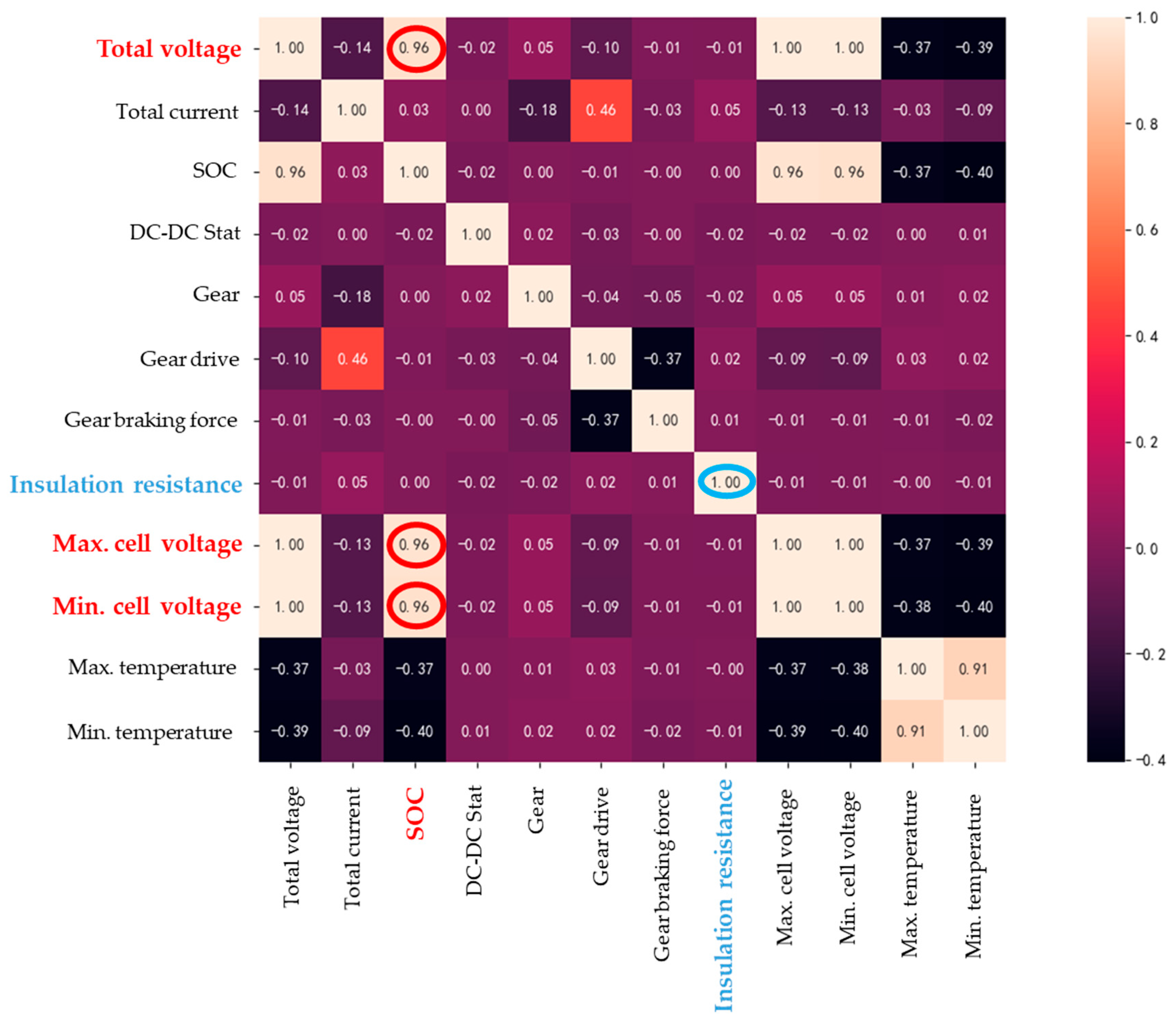
where ρ denotes the overall correlation coefficient, 𝑐𝑜𝑣(𝑋,𝑌) denotes the covariance of X and Y, and ${\sigma }_X$ and ${\sigma }_Y$ denote the standard deviation of X and Y, respectively. The range of ρ is between −1 and 1: a value closer to 1 means a higher correlation, while a value closer to −1 means a negative correlation. The correlation analysis results of the power cells in this paper are shown in Figure 4.

Based on the correlation analysis results shown in Figure 4, we can identify the characteristic parameters used to train the LSTM prediction model: the parameters strongly correlated with the SOC are total voltage, max. cell voltage, and min. cell voltage, with correlation values around 0.97. However, the correlation between insulation resistance and other battery parameters are all around 0, only with insulation resistance is there a strong correlation.

3.3. Fault Characterization

3.3.1. SOC Low Alarm Fault Characteristics

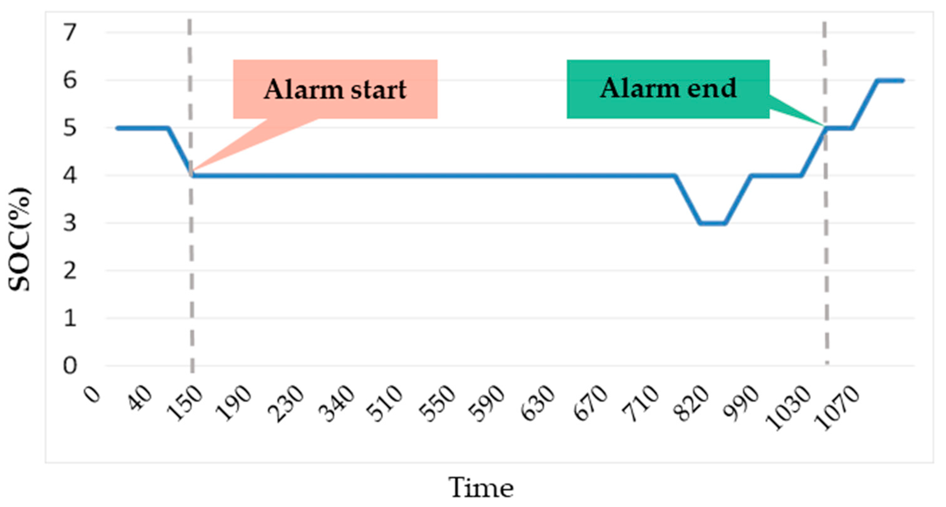
After analyzing the pre-processed vehicle operation data, the CL1 vehicle is considered as an example. The change of SOC with time is shown in Figure 5, where we can find that the vehicle battery management system (BMS) issues low SOC alarm signal conditions when the battery SOC is less than or equal to 4%. When the SOC is greater than or equal to 5%, the fault alarm is removed.

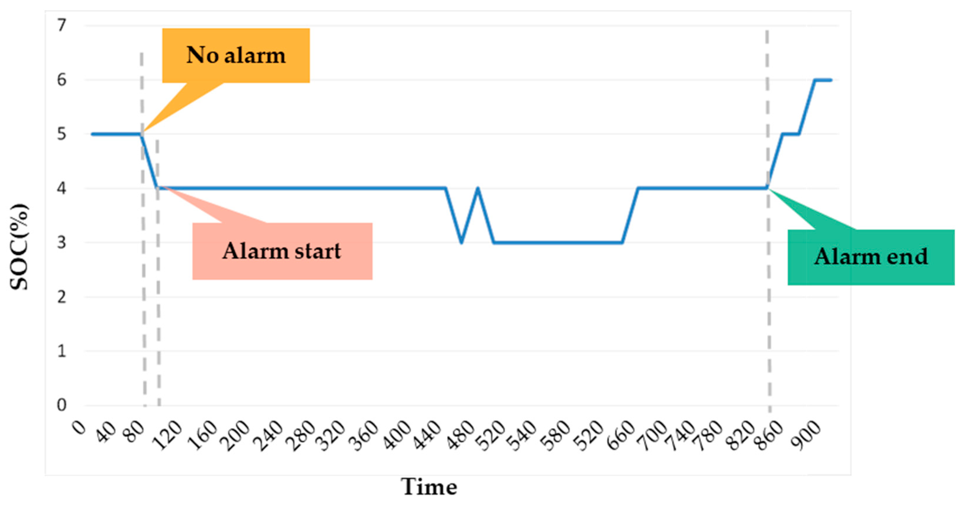
Another situation that can exist is demonstrated by considering the CL2 vehicle as an example. The corresponding SOC graph is shown in Figure 6, where the SOC value is 4% at 120 s. However, the BMS does not issue a low SOC alarm fault. We believe that this situation is caused by the rounding method used by the BMS for recording the data: the minimum SOC measurement unit is 1%, as specified in the GB/T 32960 data transmission protocol. Therefore, although the actual value of the battery SOC is between 4% and 5%, it is recorded as 4%, which does not reach the alarm threshold and, therefore, no alarm signal is issued.

After checking the operation data of the remaining vehicles, it is found that no other situation exists. In summary, we determine that the fault characteristic of a low SOC alarm is that the SOC value collected by the BMS is less than or equal to 4% after rounding. The method for predicting the occurrence of a low SOC alarm fault for the electric vehicle is by predicting the SOC of the vehicle for a future period using the online operating data of the vehicle for the previous time instant, and then predicting the possible time at which the fault can occur according to the fault characteristics.

3.3.2. Insulation Alarm Fault Characteristics

We analyzed the vehicle operation data of the insulation alarm fault, considering the CL2 data of the faulty vehicle as an example. It can be observed from Figure 7 that the insulation resistance value collected by the BMS remains basically unchanged at 1000 kΩ during the normal operation of the vehicle. The vehicle generates an alarm at 311 s, which ends at 442 s. During the alarm period, the insulation resistance value does not change significantly; however, within the 30 s before the alarm starts, the insulation resistance value changes significantly. At 279 s, the insulation resistance value changes instantaneously to 20 kΩ, and stays around this value until the alarm occurs.

The data characterization and change curve show that the insulation resistance value remains constant when the vehicle is running normally. The insulation resistance value at this time can be defined as the initial resistance value. When the insulation alarm occurs in the battery power system, the insulation resistance value deviates seriously from the initial resistance value. The fault alarm occurs 30 s after the deviation moment until the insulation resistance value returns to approximately its initial value and stabilizes for a certain period of time. Subsequently, the alarm is stopped. Therefore, the insulation alarm fault characteristics are as follows: When the ratio between the vehicle insulation resistance at a given moment and the deviation from the initial resistance is less than 1/25, the vehicle will signal a fault alarm. Note that the size of this ratio is specific to the data set used in this study.

4. Experimental Verification and Analysis

4.1. Low SOC Alarm Fault Prediction

4.1.1. Model Training and Validation

The electric vehicle low SOC fault may cause the vehicle to fail to start or move because of the remaining power battery of the vehicle being less than the set threshold value. Therefore, the prediction of a low SOC alarm fault actually predicts the SOC value of the battery. Consequently, this study transforms the problem of a low SOC alarm fault prediction into a battery SOC prediction by predicting the SOC value for a future period based on past data. Subsequently, the occurrence of a fault is predicted based on the low SOC alarm fault characteristics proposed in Section 3.3.1. A total of 1,060,962 data samples are used for the SOC prediction and the training and validation sets are divided into a ratio of 8:2.

First, the parameters window_size, batch_size and epochs of the LSTM model are randomly initialized. Subsequently, the model is run several times to obtain the optimal parameters. The value of the loss function is used as the evaluation index of the learning performance of the model. After a trial-and-error process, we gather that when the window_size is 100, batch_size is 10, and number of epochs is 5, the value of the loss function is the lowest at $1.28\times {10}^{-5}$. Any further increase in the model’s parameter values do not have any major change on the value of the loss function. Therefore, we use the above parameters as the optimal parameters for the LSTM model.

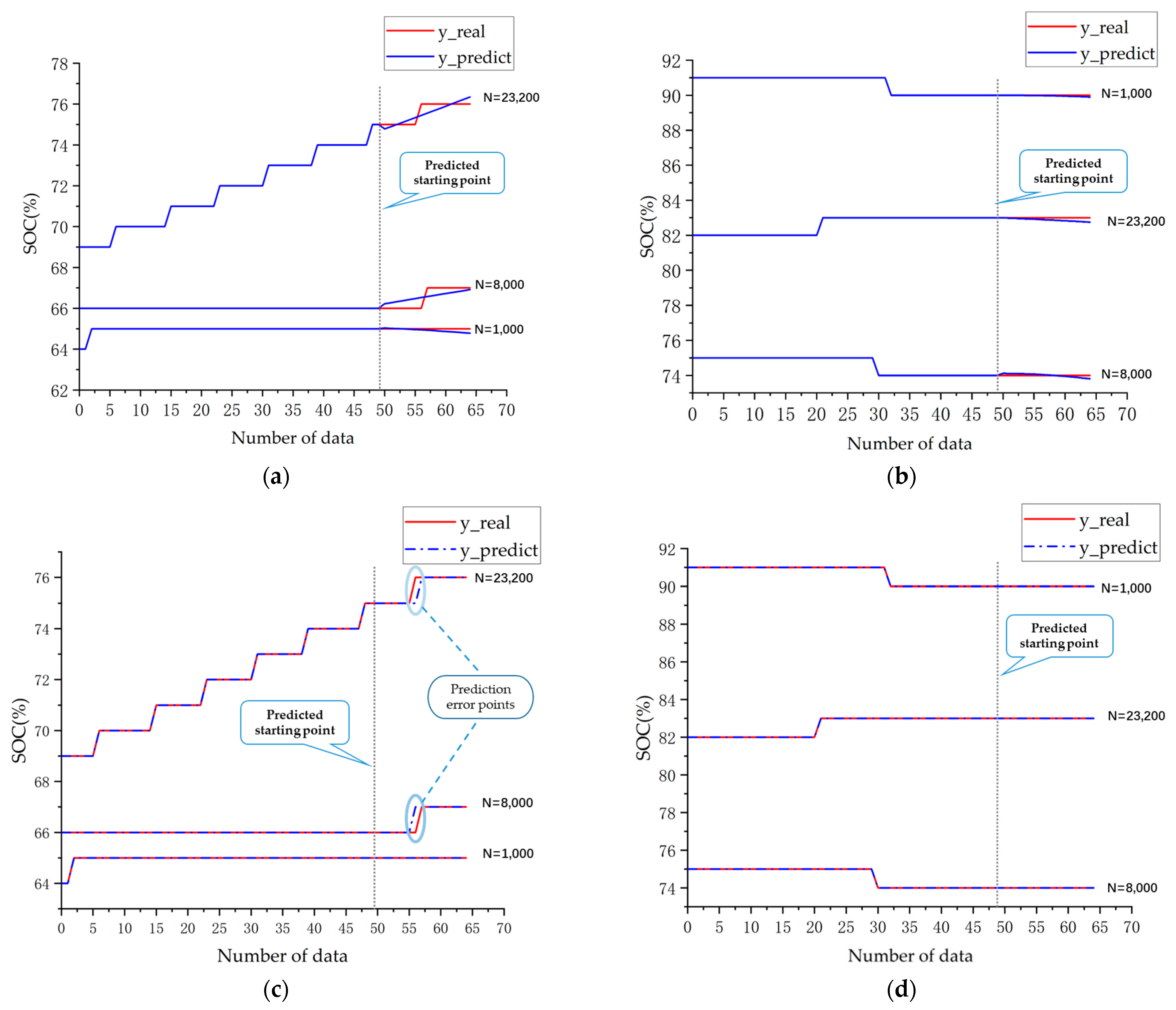
In this paper, three different positions are chosen as the starting points for prediction and predict the next 15 data points (total 300 s). From 3.2, the total voltage, the max. cell voltage, and the min. cell voltage, which are strongly correlated with the SOC, are used as the model inputs, and the SOC values are used as the outputs. The model is trained using the training sample set, and after completing the training, the model’s performance is verified using the test sample set. The corresponding results are plotted in Figure 8.

As Figure 8a,b shows, the predicted SOC values of the two models are basically equal to the actual SOC values; the two curves do not completely overlap due to the existence of fractional predicted values. After rounding the predicted values, the line graphs are plotted in Figure 8c,d. In vehicle A, only two predicted data points out of a total of 45 data points, corresponding to three different starting point positions, are not equal to the actual data points, and the rest of the data are exactly equal. In vehicle B, the 45 predicted data points are exactly identical to the actual data points, indicating that the LSTM model can effectively predict the power battery SOC values.

4.1.2. Evaluation and Analysis

In this paper, the Max Error (ME), Mean Square Error (MSE), and Root Mean Square Error (RMSE) are used to evaluate the SOC prediction performance of the LSTM models. Each index is calculated as follows:

$$ME=max\left|y_i-{\widehat{y}}_i\right|,$$

(10)

$$MSE=\frac{1}{m}{\sum }_{i=1}^m{(y_i-{\widehat{y}}_i)}^2,$$

(11)

$$RMSE=\sqrt{\frac{1}{m}{\sum }_{i=1}^m{(y_i-{\widehat{y}}_i)}^2,}$$

(12)

where m denotes the number of samples, $y_i$ denotes the true target value and ${\widehat{y}}_i$ denotes the predicted target value.

The LSTM networks prediction performance is evaluated by separately calculating the assessment indices of the three starting point positions. The results are shown in

Table 2. Summary of the evaluation indicators for different starting points.

Vehicle Type	Start Point Position	ME	MSE	RMSE
A	1000	0.220	0.0126	0.1121
	8000	0.525	0.1105	0.3324
	23,200	0.558	0.0731	0.2704
B	1000	0.102	0.0022	0.0468
	8000	0.192	0.0096	0.0979
	23,200	0.251	0.0199	0.1419

.

As Table 2 shows, the maximum ME of model A is 0.558, and the MSE and RMSE are both less than 0.4. The ME of model B is 0.25, and the MSE and RMSE are both less than 0.2. These results prove that the LSTM model can effectively learn the SOC variation and carry out SOC prediction with a lower prediction error. Therefore, the LSTM model can be used to accurately predict the vehicle’s SOC value, and diagnose the future time of vehicle failure based on the predicted value and the detection of a low SOC.

4.2. Insulation Alarm Fault Prediction

4.2.1. Model Training and Validation

The number of total samples for insulation alarm faults is 7681, with 87 fault data samples, and the ratio between the number of training set samples and validation set samples is 8:2. The optimal model parameter selection procedure is the same as that carried out for the SOC prediction. We conclude, after a trial-and-error process, that when window_size is 20, batch_size is 10, and number of epochs is 5, the value of the loss function is the lowest at $1.33\times {10}^{-5}$ and does not decrease any further. Due to the small amount of insulation alarm fault data, the window size is smaller during training in order to ensure that a better model is learnt.

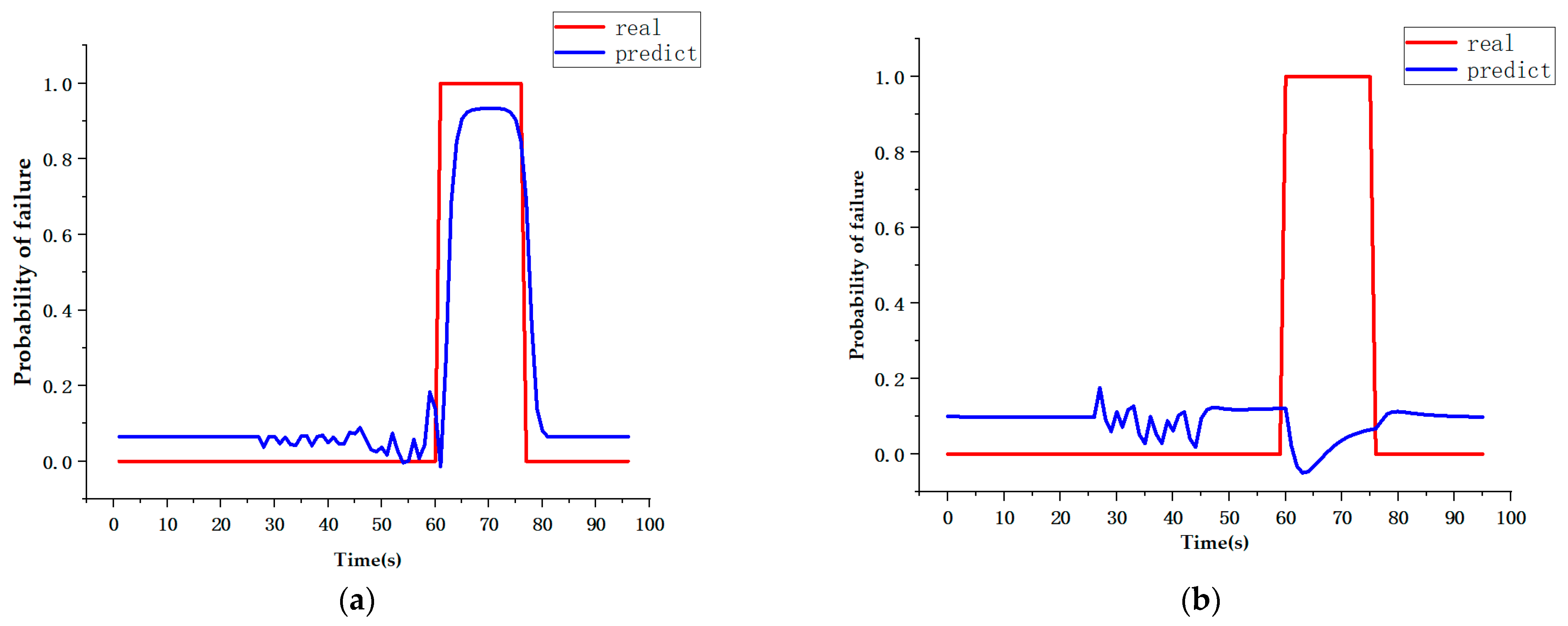
The correlation analysis presented in Section 2.2 shows that there is a parameter that is strongly correlated to the insulation resistance value. Therefore, this study uses the insulation resistance value and the occurrence of a fault alarm as the model input and predicts the fault occurrence probability as the output of the model’s training. Figure 9 shows the model’s validation results.

The figure shows that the model based on LSTM can learn the characteristics of insulation faults based on the input parameters, and the predicted fault probability is close to 1 when a fault occurs. When there is no fault, the obtained fault probability is close to 0, which indicates that the LSTM-based model can be applied to the prediction of insulation faults.

4.2.2. Evaluation and Analysis

The prediction of insulation alarm faults is similar to a classification problem. Therefore, a confusion matrix is used to define the evaluation metrics, The representation is shown in

Table 3. Parameters of the classification evaluation index.

True Value Category	Predicted Value Is Positive Example	Predicted Value Is Negative Example
Positive Example	TP	FN
Negative Example	FP	TN

:

Accuracy (ACC): This indicates the probability that the model can predict the samples that actually have faults. It is defined as follows:

$$ACC=\frac{TP+TN}{TP+TN+FP+FN},$$

(13)

True Positive Rate (TPR): This defines the probability that a fault is predicted correctly, i.e., the proportion of correct guesses in a positive sample. It can be written as

$$TPR=\frac{TP}{TP+FN},$$

(14)

False Positive Rate (FPR): This shows the probability that a fault is incorrectly predicted, i.e., the proportion of negative samples with incorrect guesses. It is expressed as follows:

$$FPR=\frac{FP}{TN+FP},$$

(15)

After the validation set was tested using the LSTM model, the sizes of the evaluation system’s indicators were recorded and these are shown in

Table 4. Real vehicle verification evaluation index parameters.

True Value Category	Predicted Value Is Positive Example	Predicted Value Is Negative Example
Positive Example	14	2
Negative Example	1	63

.

The three evaluation metrics calculated separately on the validation set are as follows: ACC is 83.75%, TPR is 87.50%, and FPR is 1.56%. The experimental results and evaluation metrics show that the LSTM model can effectively predict the probability of future failures.

5. Summary and Outlook

This paper proposed a power battery fault prediction model based on LSTM. It used the actual operation data of electric vehicles available from the online database of the new energy vehicle supervisory platform to achieve the data pre-processing, fault feature extraction, model training and prediction verification result analysis. This solution allowed the prediction of at least 15 operating features of vehicles. Consequently, the driver could be informed of the fault occurrence 150 s in advance, effectively predicting low SOC alarm faults and insulation alarm faults with an accuracy rate of more than 85%. This performance would be helpful in the safe utilization of vehicles.

However, the data used in the current study were the historical operation data of the vehicles, and there was no fault prediction based on real-time data. The next step of the study should consider embedding the model into the electric vehicle data supervision platform to process the data, to diagnose and predict fault occurrence in an online manner. At the same time, other diagnostic and prediction methods can be integrated to expand the types and robustness of the predictable faults, improve the functions of the online supervision platform, supervise vehicle operations in real-time, and help the stable development of the electric vehicle industry.

References

1. Yao, L. New energy vehicle sales exceed 6.8 million units in 2022. Auto Rev. 2023, 2, 106–107. (In Chinese) [Google Scholar]
2. Zhang, H.; Li, S.; Chen, F.; Pan, X.; Feng, H.; Sun, Y. Battery voltage fault diagnosis for electric vehicles considering driving condition variation. IET Intell. Transp. Syst. 2022, 1–17. [Google Scholar] [CrossRef]
3. Hochreiter, S.; Schmidhuber, J. Long Short-Term Memory. Neural Comput. 1997, 9, 1735–1780. [Google Scholar] [CrossRef]
4. GERS F. Long Short-Term Memory in Recurrent Neural Networks; Universität Hannover: Germany, 2001; pp. 11–14. [Google Scholar]
5. Liwicki, M.; Graves, A.; Fernandez, S.; Bunke, H.; Schmidhuber, J. A novel approach to on-line handwriting recognition based on bidirectional long short-term memory networks. In Proceedings of the 9th International Conference on Document Analysis and Recognition, ICDAR 2007, Curitiba, Brazil, 23–26 September 2007. [Google Scholar]
6. Sutskever, I.; Vinyals, O.; Le, Q.V.V. Sequence to sequence learning with neural networks. Adv. Neural Inf. Process. Syst. 2014, 27, 3104–3112. [Google Scholar]
7. Palangi, H.; Deng, L.; Shen, Y.; Gao, J.; He, X.; Chen, J.; Song, X.; Ward, R. Deep Sentence Embedding Using the Long Short Term Memory Network: Analysis and Application to Information Retrieval. arXiv 2015, arXiv:1502.06922. [Google Scholar] [CrossRef] [Green Version]
8. Karpathy, A.; Fei-Fei, L. Deep visual-semantic alignments for generating image descriptions. arXiv 2014, arXiv:1412.2306. [Google Scholar]
9. Mao, J.; Xu, W.; Yang, Y.; Wang, J.; Huang, Z.; Yuille, A. Deep captioning with multimodal recurrent neural networks (m-rnn). arXiv 2014, arXiv:1412.6632. [Google Scholar]
10. Vinyals, O.; Toshev, A.; Bengio, S.; Erhan, D. Show and tell: A neural image caption generator. arXiv 2014, arXiv:1411.4555. [Google Scholar]
11. Liu, T.; Bao, J.; Wang, J.; Zhang, Y. A Hybrid CNN–LSTM Algorithm for Online Defect Recognition of CO2 Welding. Sensors 2018, 18, 4369. [Google Scholar] [CrossRef] [Green Version]
12. Peng, Y.; Liu, X.; Wang, W.; Zhao, X.; Wei, M. Image caption model of double LSTM with scene factors. Image Vis. Comput. 2019, 86, 38–44. [Google Scholar] [CrossRef]
13. Wang, C.; Yang, H.; Meinel, C. Image captioning with deep bidirectional LSTMs and multi-task learning. ACM Trans. Multimed. Comput. Commun. Appl. (TOMM) 2018, 14, 1–20. [Google Scholar] [CrossRef]
14. Tan, Y.H.; Chan, C.S. Phrase-based image caption generator with hierarchical LSTM network. Neurocomputing 2019, 333, 86–100. [Google Scholar] [CrossRef]
15. Wen, S.; Wei, H.; Yang, Y.; Guo, Z.; Zeng, Z.; Huang, T.; Chen, Y. Memristive LSTM network for sentiment analysis. IEEE Trans. Syst. Man Cybern. Syst. 2019, 51, 1794–1804. [Google Scholar] [CrossRef]
16. Behera, R.K.; Jena, M.; Rath, S.K.; Misra, S. Co-LSTM: Convolutional LSTM model for sentiment analysis in social big data. Inf. Process. Manag. 2021, 58, 102435. [Google Scholar] [CrossRef]
17. Wang, H.; Zhang, X.; Liang, B.; Zhou, Q.; Xu, B. Gated hierarchical LSTMs for target-based sentiment analysis. Int. J. Softw. Eng. Knowl. Eng. 2018, 28, 1719–1737. [Google Scholar] [CrossRef]
18. Jiang, H.; Jiao, R.; Wang, Z.; Zhang, T.; Wu, L. Construction and analysis of emotion computing model based on LSTM. Complexity 2021, 2021, 8897105. [Google Scholar] [CrossRef]
19. Huang, F.; Li, X.; Yuan, C.; Zhang, S.; Zhang, J.; Qiao, S. Attention-emotion-enhanced convolutional LSTM for sentiment analysis. IEEE Trans. Neural Netw. Learn. Syst. 2021, 33, 4332–4345. [Google Scholar] [CrossRef]
20. Saadatnejad, S.; Oveisi, M.; Hashemi, M. LSTM-based ECG classification for continuous monitoring on personal wearable devices. IEEE J. Biomed. Health Inform. 2019, 24, 515–523. [Google Scholar] [CrossRef] [Green Version]
21. Wójcikowski, M. Real-time PPG signal conditioning with long short-term memory (LSTM) network for wearable devices. Sensors 2021, 22, 164. [Google Scholar] [CrossRef]
22. Ye, Z.; Yu, J. Health condition monitoring of machines based on long short-term memory convolutional autoencoder. Appl. Soft Comput. 2021, 107, 107379. [Google Scholar] [CrossRef]
23. Li, Z.; Jiang, W.; Wu, X.; Zhang, S.; Chen, D. Study on Health Indicator Construction and Health Status Evaluation of Hydraulic Pumps Based on LSTM–VAE. Processes 2022, 10, 1869. [Google Scholar] [CrossRef]
24. Kim, H.; Kwon, Y.; Choi, Y. Assessing the impact of public rental housing on the housing prices in proximity: Based on the regional and local level of price prediction models using long short-term memory (LSTM). Sustainability 2020, 12, 7520. [Google Scholar] [CrossRef]
25. Bathla, G.; Rani, R.; Aggarwal, H. Stocks of year 2020: Prediction of high variations in stock prices using LSTM. Multimed. Tools Appl. 2023, 82, 9727–9743. [Google Scholar] [CrossRef]
26. Li, R.; Hu, Y.; Liang, Q. T2F-LSTM method for long-term traffic volume prediction. IEEE Trans. Fuzzy Syst. 2020, 28, 3256–3264. [Google Scholar] [CrossRef]
27. Hong, J.; Wang, Z.; Yao, Y. Fault prognosis of battery system based on accurate voltage abnormity prognosis using long short-term memory neural networks. Appl. Energy 2019, 251, 113381. [Google Scholar] [CrossRef]
28. Zhang, H.; Niu, G.; Zhang, B.; Miao, Q. Cost-effective lebesgue sampling long short-term memory networks for lithium-ion batteries diagnosis and prognosis. IEEE Trans. Ind. Electron. 2021, 69, 1958–1967. [Google Scholar] [CrossRef]
29. Ding, X.; Cui, Z.; Yuan, H.; Cui, N. Diagnosis of connection fault for parallel-connected lithium-ion batteries based on long short-term memory networks. J. Energy Storage 2022, 55, 105552. [Google Scholar] [CrossRef]
30. Trivedi, M.; Kakkar, R.; Gupta, R.; Agrawal, S.; Tanwar, S.; Niculescu, V.C.; Raboaca, M.S.; Alqahtani, F.; Saad, A.; Tolba, A. Blockchain and Deep Learning-Based Fault Detection Framework for Electric Vehicles. Mathematics 2022, 10, 3626. [Google Scholar] [CrossRef]
Figure 1. Schematic diagram of the RNN network structure.
Energies 16 04733 g001
Figure 2. Schematic of the LSTM structure.
Energies 16 04733 g002
Figure 3. Fault prediction process diagram.
Energies 16 04733 g003
Figure 4. Graph of the correlation analysis results.
Energies 16 04733 g004
Figure 5. CL1 SOC variation graph.
Energies 16 04733 g005
Figure 6. CL2 SOC variation graph.
Energies 16 04733 g006
Figure 7. CL2 vehicle insulation resistance curve.
Energies 16 04733 g007
Figure 8. SOC prediction results. (a) Vehicle A; (b) Vehicle B; (c) Vehicle A rounding result chart; (d) Vehicle B rounding result chart.
Energies 16 04733 g008
Figure 9. (a) Real vehicle verification performance; (b) Ineffective prediction schematic.
Energies 16 04733 g009