PV Temperature Prediction Incorporating the Effect of Humidity and Cooling Due to Seawater Flow and Evaporation on Modules Simulating Floating PV Conditions

Abstract

The temperature prediction for floating PV (FPV) must account for the effect of humidity. In this work, PV temperature prediction for steady-state T_pv and transient conditions T_pv(t) incorporates the effect of humidity and cooling due to seawater (s.w.) splashing and evaporation on PV modules. The proposed formulas take as main inputs the in-plane solar irradiance_, wind speed, ambient temperature, relative humidity (RH), and s.w. temperature. The transient effects of s.w. splashing and the evaporation of the s.w. layer from the module are theoretically described considering the layer’s thickness using Navier–Stokes equations. T_pv and T_pv(t) measurements were taken before and after s.w. splashing on c-Si modules at the seashore and inland. PV temperature predictions compared to measured values showed very good agreement. The 55% RH at the seashore versus 45% inland caused the T_pv to decrease by 18%. The T_pv(t) at the end of the s.w. flow of 50–75 mL/s/m on the module at the seashore was 35–51% lower than the T_pv inland. This T_pv(t) profile depends on the s.w. splashing, lasts for about 1 min, and is attributed to higher convection, water cooling, and evaporation on the modules. The PV efficiency at FPV conditions was estimated to be 4–11.5% higher compared to inland.

1. Introduction

It is well established that when solar irradiance, I_T, impinges on a PV module, a small part is reflected, while the main part is transmitted and absorbed. The latter is converted into power with efficiency η_pv and the rest is degraded into heat, which increases the PV cell temperature, T_pv, above the ambient temperature, T_a. The steady-state PV temperature, as well as the T_pv(t) profile at transient conditions for modules operating on land, has been extensively studied through simulation models taking into consideration wind speed and the effect of PV temperature through implicit functions [1,2,3], the varying environmental conditions [4,5,6,7], and also the PV module inclination and orientation with reference to the wind direction [8,9]. These models were primarily developed for land-based PV (LBPV), resulting in a generally good agreement between predicted and measured values. The effect of the environmental conditions on T_pv, and hence on P_m in c-Si modules, was further investigated theoretically and experimentally to cover a wide range of mounting configurations, PV technologies, and years of operation, and a model for T_pv prediction was developed in [10], achieving a very high accuracy for any PV installations that were free-standing, building-integrated PV (BIPV), or building-adapted PV (BAPV), and also incorporated the effect of aging. Other empirical and semi-empirical formulas that predict T_pv and T_pv(t) have been proposed and validated in a large diversity of PV configurations [11,12,13,14], while formulas based on artificial neural networks (ANNs) [15,16,17] predicted T_pv for FPV installations studied for each case. T_pv is a crucial factor that affects efficiency, η_pv, and evidently the PV power output, P_m, [18], while high T_pv and humidity accelerate the PV cell’s aging [19,20,21,22]. In the last decade, the study of the PV performance in lakes and reservoirs, nearshore and offshore, has been given special attention because of interest in floating PV (FPV) [23,24,25,26], with a focus on the effect of the environmental conditions, such as I_T, wind speed, v_w, ambient temperature, T_a, seawater (s.w.) temperature, T_s.w., humidity, hu, and salinity on T_pv, accounting for the different values those parameters take inland and on the seashore/offshore [27,28]. The induced PV cooling to partially recover P_m losses from the effect of T_pv has been studied using various techniques. Heat extraction by means of water flowing on the front PV side [29,30,31,32] was reported to cause a T_pv decrease of 20%, which increased with the flow rate. The water jet impingement or spray on the front and/or back PV sides [33,34] resulted in 14% recuperation of the power losses. PV cooling using either a soaked sponge or water spraying on the PV backside was reported to lead to the recuperation of P_m losses greater than 28% [35,36,37].

FPV installations in near-shore environments exposed to high hu and salinity showed a boost in performance vs. LBPV [23,24,26]. Recent works focus on the effect of the I_T, v_w, T_a, T_s.w., hu, salinity, and FPV installation geometries on T_pv. The prospects and challenges of various types of modules in FPV installations were discussed in [25,38,39,40], while the impact of climatic conditions, with a special emphasis on FPV, was estimated in [41,42] and in the tropics in [43,44,45] using simulation models. The estimation of T_pv in FPV plants was further studied in [46,47,48,49] with an emphasis on the impact of hu [50,51,52] and the effect of the solar spectral irradiance on the PV yield in [53].

Generally, the T_pv prediction formulae incorporated the heat loss coefficient, U_pv, for FPV systems that were either air-cooled or air/water-cooled [45,46,47], while the hu effect was not considered explicitly. In [47], two FPV-mounting technologies were compared, and T_pv was found to be lower in air-cooled FPV than in the FPV in direct contact with water. The larger drop in the T_pv for the air-cooled FPV was attributed to the higher v_w. In [41], T_pv was determined to be 9–14 °C lower in the sea environment (s.e.) compared to inland in two climatic conditions, the Netherlands (NL) and Singapore (SG). T_pv was found to be 13 °C lower in large- and medium-footprint FPV compared to rooftop PV in SG and by 11 °C lower in offshore FPV compared to LBPV in the NL due to higher v_w and hu in the s.e. Other effects on T_pv due to solar irradiance spectrum [27], FPV mounting geometry [41], air/water environmental quantities [28] using appropriate databases, and the evaporation from the sea surface [54] and the PV module must be considered. It is important to note the lower albedo at s.e., about 8% compared to 15% on the ground [38,44,45]. However, due to the low tilt of the modules in the s.e., the effect of albedo is not significant.

The above literature review addresses the following main issues:

• The Effect of RH on T_pv

T_pv decreases as RH increases [43,49], while [48] concludes that RH does not play an important role in the performance of the T_pv and PV. On the contrary, in [50,52], it is claimed that T_pv increases with RH and P_m decreases. However, in low RH, the PV performance may also increase with RH based on the combined effect of the environmental quantities given in [49,50,51]. The aforementioned findings are opposite, justifying the need for a further investigation of the effect of RH on T_pv.

2.

The Combined effect of wind and water on T_pv

Τ_pv in FPV was found to be 5–10 °C lower than in LBPV due to the cooling effect of the water evaporation and the higher v_w [44,46,47,48]. Comparing FPV and LBPV in the NL and SG in [41], it was found that T_pv was 3.2 °C lower in FPV at s.e. vs. LBPV in the NL and 14.5 °C lower at s.e. vs. rooftop PV in SG. Additionally, in the aforementioned study, it was found that RH was 4.7% higher in s.e. than in rooftop PV in nearby sites, where T_a was 1–1.2 °C lower in s.e. and v_w was 1 m/s higher due to lower air friction.

3.

Spectral effects

T_pv is affected by the spectrum shift towards the red due to solar light scattering on aerosol molecules. As the humid environment causes a spectrum redshift, which corresponds to the infrared part of the spectrum, the performance of c-Si FPV might be lower than the LBPV considering that c-Si PV have a spectral response in the 300–1100 nm range. Thin film technologies such as a-Si or CdTe are less affected by the redshift as their spectral response is mainly in the visible part of the spectrum [18,51].

4.

Atmospheric effects

The FPV performance was found to be 12.96% higher in the s.e. than the LBPV [49]. The global horizontal irradiation was about 8.54% higher in the s.e. because the sky above the sea is in general clearer than over the green land. The transparency of the atmosphere depends on the combined effect of T_a, T_s.w., v_w, and air and water vapor pressure. Aerosols and air moisture shift the light spectrum towards the red and may attenuate I_T in a rich s.w. evaporation area with low v_w or when wind transfers water droplets in the air. This has a negative effect, decreasing I_sc and P_m [44,46,52,53]. On the contrary, the convection coefficient, h_c, increases with hu, causing a T_pv decrease (positive effect) [15,16,49]. These opposite effects may be the reason the T_pv results in the FPV installations do not always agree, as mentioned in point 1 above.

5.

T_pv modeling in FPV

A T_pv prediction model for FPV is outlined in [48], where the effect of T_s.w. is indirectly accounted for in the U_pv estimation, whereas the effect of v_w and hu is not incorporated. For FPV of various water footprints, U_pv was estimated as 27 W/m²K inland, 37 W/m²K near-shore, and 57 W/m²K offshore [46,47]. In [16], it is stated that the existing models overestimate T_pv in s.e. because the cooling effect on PV through T_s.w. and hu is not accounted for. The correlation between T_pv and RH is considered through either regression analysis [43] or ANN where, depending on the PV cell type and the site conditions, RH has either a positive or negative effect on T_pv [15].

FPV Research Gaps and Objectives

Natural PV cooling due to the increased hu on the seashore/near-shore/offshore, along with the different values in the environmental parameters between inland and seashore/offshore, as well as the seawater splashing on the modules and the evaporation on their surface have not been rigorously studied, especially as it concerns their effect on T_pv and η_pv. This paper fills in gaps in the literature as it concerns the natural and induced PV cooling of modules operating in the s.e. A robust theoretical analysis on the effect of RH, s.w. temperature, s.w. splashing on the modules, and the s.w. layer evaporation on the front side of the modules on the transient T_pv(t) profile is outlined. A complete set of formulas is elaborated to predict T_pv, expanding the previous work of the authors [10], taking into account the effect of hu and indirectly of T_s.w. or freshwater temperature T_w. For the validation of the model, the predicted T_pv values are compared to the measured ones inland and on the seashore and compared further to T_pv values produced using other formulas proposed in [14,15,16,43,48].

2. Experimental Procedure for the Measurement of the T_pv Profiles on the Seashore and Inland

The steady-state temperature T_pv and the temperature profile T_pv(t) on the front side, also denoted as T_f(t), of mono c-Si M55 modules operating for 24 years with η_pv = 0.095 due to ageing, and mono c-Si SW80 modules with η_pv = 0.146, were measured at two sites. The modules were placed facing South with inclination β = 35° on the seashore at latitude φ = 38.311° N and L = 21.78° E and on the terrace of a building inland, φ = 38.22° N and L = 21.75° E. T_pv was measured in March under a bright environment with high air visibility and no water drops or water layer deposited on the PV modules, at RH equal to 55% on the seashore and 45% inland. The experiments were carried out at around solar noon under I_T = 800 W/m². The steady-state front side PV temperature, T_f = T_pv, was measured around the middle on one of the cells.

The study of the PV cooling included s.w. flow on the inclined module, simulating s.w. splashing on the module. T_s.w. was 14–15 °C during the experiments. The steady-state T_pv was measured prior to the s.w. flow on the module. The s.w. volume flow rate, Q, per unit width b, (Q/b), was 40, 50, and 75 mL/s/m and was sustained for a period of 2 to 6 s depending on the experiment. The measurement of the transient profile T_f(t) = T_pv(t) of the s.w. layer on the module began when the s.w. flow on the module stopped and continued until the layer was totally evaporated. The research focused on the effect of hu on T_pv under a clear sky and the effect of the s.w. flow on the module and the subsequent s.w. layer evaporation from its front side.

The environmental conditions at the time of the experiments were measured with the following sensors. A Kipp & Zonen CMP11 pyranometer (ISO 9060 & IEC 61724 Class A) coupled to a METEON data logger with an accuracy of 0.1% was used for the intensity, I_T, on the PV plane. T_a and RH were measured using a thermohygrometer with an accuracy of ±0.5 °C for the T_a and ±2% for the RH. The PV temperature T_f(t) = T_pv(t) was measured using a TROTEC TP10 IR thermometer with an accuracy of ±1 °C. The wind speed v_w was measured using a Sefram 9862 hot wire anemometer with an accuracy of ±3%. During the measurements, v_w varied by 0.5 m/s which caused variation in the T_pv of ±1 °C. This band is the same as the accuracy of the temperature sensor TROTEC TP10 used in the measurements. An error analysis of T_pv prediction, taking into account the error in the measurement of the input parameters, is given in Section 4.3.

3. Theoretical Analysis of T_pv Profiles on the Seashore vs. Inland

The effect of hu on T_pv and also the T_pv(t) profiles due to s.w. splashing on a module and the s.w. evaporation from the module front side were studied theoretically and applied in the measurement scenarios for modules operating on the seashore and inland.

The steady-state PV temperature was predicted by incorporating a humidity correction factor improving the T_pv prediction formula previously proposed for free-standing, BIPV/BAPV [10], and adapting it to the s.e., freshwater environment, as well as humid inland environments.

The T_pv(t) = T_f(t) profile was studied considering conduction, convection, and s.w. layer evaporation on the module, while the s.w. layer’s thickness was estimated by solving the Navier–Stokes equation. These heat and mass flow processes were considered in the study of the T_pv(t) profiles as they contribute towards the heat extraction from the modules.

3.1. Steady-State T_pv Prediction Model

For modules operating inland or in the s.e. under the conditions of I_T, T_a, v_w, T_s.w., RH, and inclination β, T_pv may be predicted through the following set of formulas. Generally,

T_pv = T_a + f·I_T

(1)

A generalized form of the coefficient f, known in its simplest form as the Ross coefficient in Equation (1), is predicted for any PV mounting configuration by Equations (2a,b) and (3), which hold for an average RH = 45%, based on the previous work of the authors [10]:

$$\mathrm{f}=\mathrm{f}\left({\mathrm{v}}_{\mathrm{w}}\right)\left(1-\frac{\left(\left(\frac{{\mathsf{\vartheta }\mathsf{\eta }}_{\mathrm{p}\mathrm{v}}}{\mathsf{\vartheta }{\mathrm{T}}_{\mathrm{p}\mathrm{v}}}\right)\mathsf{\delta }{\mathsf{{\rm T}}}_{\mathrm{p}\mathrm{v}}+\left(\frac{{\partial \mathsf{\eta }}_{\mathrm{p}\mathrm{v}}}{{\partial \mathrm{I}}_{\mathrm{T}}}\right)\mathsf{\delta }{\mathrm{I}}_{\mathrm{T}}\right)}{\left(1-{\mathsf{\eta }}_{\mathrm{p}\mathrm{v},\mathrm{S}\mathrm{O}\mathrm{C}}\right)}\right)\left(1-\frac{\left(\frac{{\partial \mathrm{U}}_{\mathrm{f}}}{\partial {\mathrm{T}}_{\mathrm{p}\mathrm{v}}}\right)\mathsf{\delta }{\mathsf{{\rm T}}}_{\mathrm{p}\mathrm{v}}+\left(\frac{{\partial \mathrm{U}}_{\mathrm{b}}}{\partial {\mathrm{T}}_{\mathrm{p}\mathrm{v}}}\right)\mathsf{\delta }{\mathrm{T}}_{\mathrm{p}\mathrm{v}}+\left(\frac{{\partial \mathrm{U}}_{\mathrm{f}}}{\partial \mathsf{\beta }}\right)\mathsf{\delta }\mathsf{\beta }+\left(\frac{{\partial \mathrm{U}}_{\mathrm{b}}}{\partial \mathsf{\beta }}\right)\mathsf{\delta }\mathsf{\beta }}{{\mathrm{U}}_{\mathrm{p}\mathrm{v},\mathrm{S}\mathrm{O}\mathrm{C}}}\right)$$

(2a)

$$\mathrm{f}=\mathrm{f}\left({\mathrm{v}}_{\mathrm{w}}\right)\left(1-\frac{\left(\frac{{\mathsf{\vartheta }\mathsf{\eta }}_{\mathrm{p}\mathrm{v}}}{\mathsf{\vartheta }{\mathrm{T}}_{\mathrm{p}\mathrm{v}}}\right)\mathsf{\delta }{\mathrm{T}}_{\mathrm{p}\mathrm{v}}+\left(\frac{{\partial \mathsf{\eta }}_{\mathrm{p}\mathrm{v}}}{{\partial \mathrm{I}}_{\mathrm{T}}}\right)\mathsf{\delta }{\mathsf{{\rm I}}}_{\mathsf{{\rm T}}}}{1-{\mathsf{\eta }}_{\mathrm{p}\mathrm{v},\mathrm{S}\mathrm{O}\mathrm{C}}}\right)$$

(2b)

Equation (2a) holds for natural flow or v_w < 1.5 m/s, and Equation (2b) holds for air-forced flow or v_w > 1.5 m/s.

$\mathrm{f}\left({\mathrm{v}}_{\mathrm{w}}\right)$ expresses the impact of wind speed on the f coefficient and is given by:

$$\mathrm{f}\left({\mathrm{v}}_{\mathrm{w}}\right)=\frac{\mathrm{a}+{\mathrm{b}\mathrm{v}}_{\mathrm{w}}}{1+{\mathrm{c}\mathrm{v}}_{\mathrm{w}}+{\mathrm{d}\mathrm{v}}_{\mathrm{w}}^2}$$

(3)

where a = 0.0375, b = 0.0081, c = 0.2653, and d = 0.0492 [10].

Equation (2a,b) is expressed through the multiplication of $\mathrm{f}\left({\mathrm{v}}_{\mathrm{w}}\right)$ with correction factors due to the deviation of the efficiency η_pv from a reference value at standard operating conditions (SOCs) and the effect of the PV temperature and module inclination on the heat losses coefficients in the front and back side of the modules, U_f and U_b, respectively. The factors η_pv,soc, U_pv,soc, dη_pv/dT, dη_pv/dI_T, dU_f/dT, dU_b/dT, dU_f/dβ, and dU_b/dβ are defined and determined in [10].

In the present work, the applicability of the above expression is extended to the s.e., freshwater environment, and humid inland environment, with the introduction of a new correction factor in the model for f, expressing the effect of RH and T_s.w. or T_w on T_pv.

The humidity affects the convection coefficient h_c due to the higher dynamic viscosity of H₂O. The h_c,a with dry air as a coolant vs. h_c,s.w. with s.w. as a coolant may be expressed through the ratio of their corresponding Nu number [55]. The ratio h_c,a/h_c,s.w. is practically estimated by Equations (4)–(6) to account for the effect of hu on h_c. The deviation of RH from its reference value 45% causes a change in δh_c or δU_pv to be introduced in the prediction of f and T_pv as outlined below. Equations (4) and (5) stand for turbulent and laminar forced flow over a flat surface, respectively, and Equation (6) holds for natural heat transfer.

h_c,a/h_c,s.w. = (k_a/k_s.w.)·(Pr_a/Pr_s.w.)^1/3·(ν_a/ν_s.w.)^0.8 forced flow, turbulent, Re > 5 × 10⁵

(4)

h_c,a/h_c,s.w. = (k_a/k_s.w.)·(Pr_a/Pr_s.w.)^1/3·(ν_a/ν_s.w.)^1/2 laminar forced flow, Re < 5 × 10⁵

(5)

h_c,a/h_c,s.w. = (k_a/k_s.w.)·(Pr_a/Pr_s.w.)^1/3·(ν_a/ν_s.w.)^1/3 for natural heat flow

(6)

where k_a and k_s.w. are the thermal conductivity of air and s.w., respectively, in (W/mK); ν_a and ν_s.w. are the kinematic viscosity of air and s.w., respectively, in (m²/s); and Pr_a and Pr_s.w. are the Prandtl numbers of air and s.w., respectively.

The difference in h_c is estimated by Equation (7a,b) for the following cases:

• RH₁ (p_hu,1% moles of dry air and q_hu,1% moles of H₂O), with p_hu,1 + q_hu,1 = 1.
• RH₂ (p_hu,2% moles of dry air and q_hu,2% moles of H₂O), with p_hu,2 + q_hu,2 = 1.

h_c,2 − h_c,1 = (p_hu,2 − p_hu,1)·h_c,a + (q_hu,2 − q_hu,1)·h_c,H2O

(7a)

δh_c,hu = δp_hu·h_c,a + δq_hu·h_c,H2O

(7b)

δp_hu and δq_hu denote the difference in p_hu and q_hu at two different conditions where RH differs. These are determined from the Mollier diagrams.

The new correction factor for coefficient f is presented in Equation (8). It accounts for the effect of the difference between RH_s.e. and RH_inl and gives the f_s.e. for the s.e. in relation to f_inl for inland, where RH = 45%. The correction term δh_c,hu/U_pv is estimated by Equation (7b), while U_pv = h_c,f + h_c,b + h_r,f + h_r,b is estimated as outlined in [8,10].

f_s.e. = f_inl·(1 − δh_c,hu/U_pv)

(8)

The above correction factor is introduced through the last term (1 − δh_c,hu/U_pv) in Equation (9), improving the previous holistic model for f [10].

$$\mathrm{f}=\mathrm{f}\left({\mathrm{v}}_{\mathrm{w}}\right)\left(1-\frac{{\mathsf{\delta }\mathsf{\eta }}_{\mathrm{p}\mathrm{v}}}{\left(1-{\mathsf{\eta }}_{\mathrm{p}\mathrm{v},\mathrm{S}\mathrm{O}\mathrm{C}}\right)}\right)\left(1-\frac{{\mathsf{\delta }\mathrm{U}}_{\mathrm{p}\mathrm{v}}}{{\mathrm{U}}_{\mathrm{p}\mathrm{v},\mathrm{S}\mathrm{O}\mathrm{C}}}\right)\left(1-\frac{{\mathsf{\delta }\mathsf{\eta }}_{\mathrm{a}\mathrm{g}}}{\left(1-{\mathsf{\eta }}_{\mathrm{p}\mathrm{v},\mathrm{S}\mathrm{O}\mathrm{C}}\right)}\right)\left(1-\frac{{\mathsf{\delta }\mathsf{\eta }}_{\mathrm{t}\mathrm{e}\mathrm{c}}}{\left(1-{\mathsf{\eta }}_{\mathrm{p}\mathrm{v},\mathrm{S}\mathrm{O}\mathrm{C}}\right)}\right)\left(1-\frac{{\mathsf{\delta }\mathrm{h}}_{\mathrm{c},\mathrm{h}\mathrm{u}}}{{\mathrm{U}}_{\mathrm{p}\mathrm{v},\mathrm{S}\mathrm{O}\mathrm{C}}}\right)$$

(9)

Note that the second correction term $\left(1-\frac{{\mathsf{\delta }\mathrm{U}}_{\mathrm{p}\mathrm{v}}}{{\mathrm{U}}_{\mathrm{p}\mathrm{v},\mathrm{S}\mathrm{O}\mathrm{C}}}\right)$ applies only for natural flow (or v_w < 1.5 m/s) and is omitted for turbulent flow (or v_w > 1.5 m/s). The third and fourth correction terms describe the impact of ageing and PV technology/efficiency, respectively, as outlined in [10].

The introduction of the last term $\left(1-\frac{{\mathsf{\delta }\mathrm{h}}_{\mathrm{c},\mathrm{h}\mathrm{u}}}{{\mathrm{U}}_{\mathrm{p}\mathrm{v},\mathrm{S}\mathrm{O}\mathrm{C}}}\right)$ accounts for the effect of hu and T_s.w. or T_w as per case in the prediction of T_pv and applies to FPV both at s.w. and freshwater environments as well as LBPV at RH conditions different than 45%.

3.2. Transient Effects in T_pv Due to Water Splashing on the PV Module

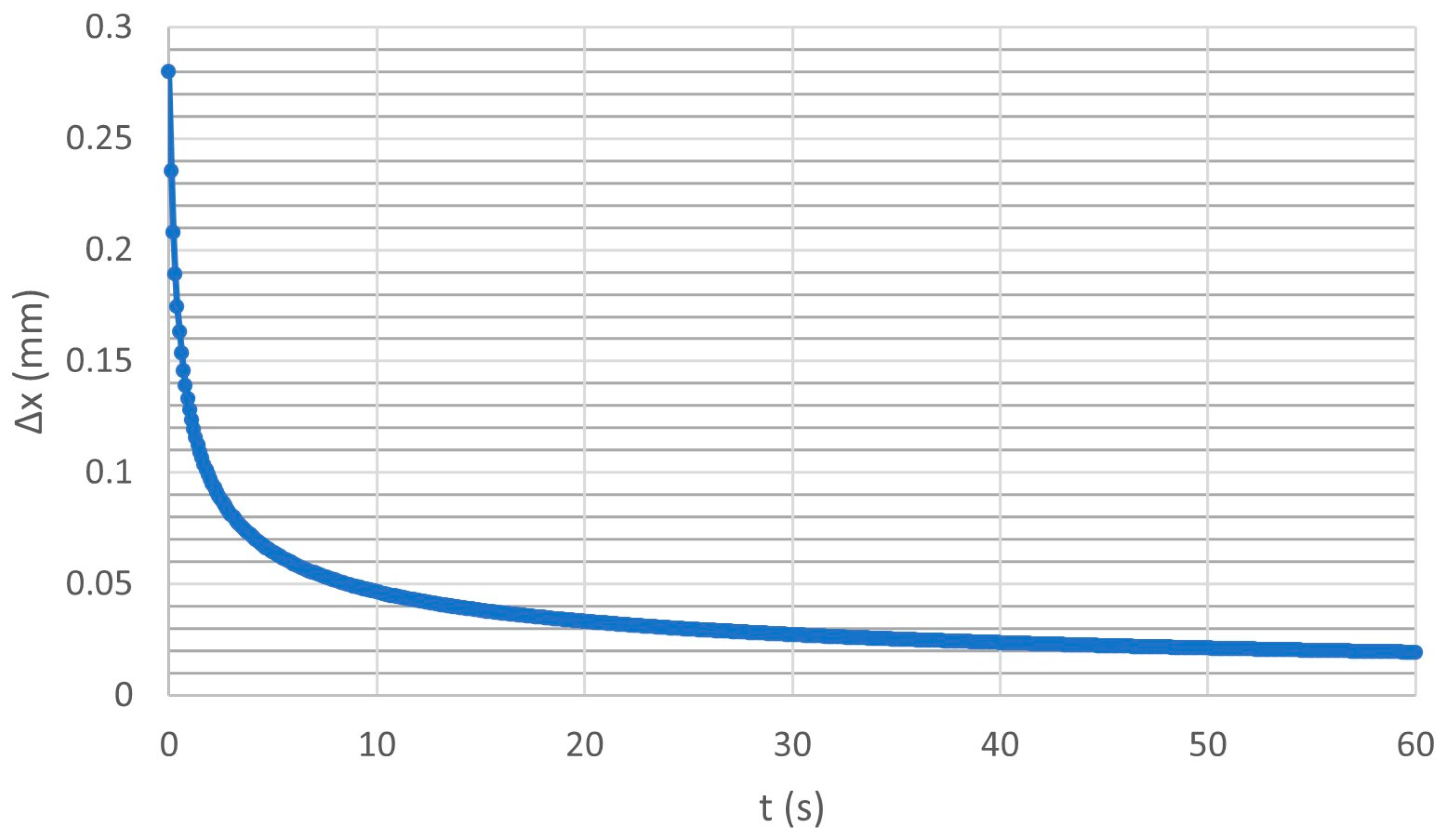
3.2.1. Seawater Layer Thickness

Let Δx_o be the thickness of the s.w. layer which flows steadily on an inclined module. Due to gravitational forces, when the flow stops, the thickness of the s.w. layer becomes thinner with time, Δx(t). Assuming fully developed laminar flow, both Δx_o and the s.w. layer velocity profile, u(y), are determined by the Navier–Stokes equations for a Newtonian non-compressible fluid at steady-state flow on the module; see Equations (10)–(14) [55,56]. y is the distance measured from the module plane along a y-axis normal to the PV plane, where 0 < y < Δx.

0 = νd²u(y)/dy² + ρ g sin(β) = 0

(10)

For boundary conditions u(y = 0) = 0 and du/dy = 0 at y = Δx:

u(y) = (gsin(β)/ν) (yΔx − y²/2)

(11)

The volume flow rate Q per unit width b, that is the width of the string of PV cells in a module over which s.w. flows, is given by Equation (12), while Δx_o is given by Equation (13).

$$\mathrm{Q}/\mathrm{b}={\int }_0^{\mathsf{\Delta }{\mathrm{x}}_{\mathrm{o}}}\mathrm{u}\left(\mathrm{y}\right)\mathrm{d}\mathrm{y}$$

(12)

Δx_o = [3ν·Q/(b·g·sin(β))]^1/3

(13)

where ν is the s.w. kinematic viscosity obtained from the literature. Substituting ν, Q/b, and β into Equation (13) gives Δx_o equal to 0.32 mm and 0.37 mm corresponding to Q/b = 50 and 75 mL/s/m, respectively, for s.w. at 14 °C, while Δx_o = 0.28 mm and 0.32 mm, respectively, for the s.w. layer of T_s.w. = 30 °C. Δx(t) thins exponentially when the s.w. stops flowing according to Equation (14) [57], and so its contribution to heat capacity becomes negligible soon.

d(Δx)/Δx = −u_av t/l

(14)

Δx(t + δt) = Δx(t)exp(−u_av(t)·δt/l)

(15)

where l is the length along the s.w. flow with l = 0.1 m where T_f(t) was measured. u_av is the average s.w. layer velocity at l when s.w. flows down the module and is a function of t. Equations (11)–(13) provide u_av(t), where:

u_av(t) = gsinβ(Δx(t))²/3ν_f

(16)

The subscript f denotes that the value of ν corresponds to T_f. Δx in Equation (15) holds when the viscous forces and surface tension, σ, are low compared to gravitational forces. This holds for Δx bigger than a critical value, h_cr [57]:

h_cr = 2dσ/dz(1 − cosθ)/ρg

(17)

where θ = 107° is the contact angle of the water–glass interface. dσ/dz is the derivative of the surface tension taken equal to σ/L_pv, with L_pv = 1.2 m corresponding to the length of the module, and z is an axis along the inclined module. Therefore, dσ/dz = 73.477 × 10⁻³ N/m/m at T_s.w. = 30 °C and salinity 35 g/kg. Substituting these values in Equation (17) gives h_cr = 0.019 mm.

For t = 0 when Δx = Δx_o, u_av is estimated equal to 0.157 m/s at T_s.w. = 14 °C, and 0.175 m/s at T_s.w. = 30 °C. u_av is negligible at thickness h_cr. Δx(t) and u_av(t) are determined at l = 0.1 m in steps of δt = 0.1 s following iteration between Equations (15) and (16). The results are shown in Figure 1. Δx reaches the h_cr value at around 60 s, where the water film shows no motion because viscous forces and surface tension between water and glass prevail.

3.2.2. T_pv(t) Profile Taking into Consideration the s.w. Layer on the PV

The transient T_pv(t) profile due to s.w. splashing is expected to experience an initial steep drop. The time constant τ_s.w. of the heat convection due to the s.w. layer on the module is determined by Equation (18). Introducing into Equation (18), the s.w. density ρ, its heat capacity c_p, the total heat transfer coefficient U_pv, and Δx_o, τ_s.w. is estimated to be 57 s at the beginning of the phenomenon.

τ_s.w. = ρ Δx cp/U_pv

(18)

The heat conduction acts directly in full strength in such thin layers. The initial T_pv drop may be estimated applying the continuity in the heat conduction flow along a y-axis normal to the boundary between the PV glass and the s.w. layer, Equation (19), [56].

k_gl dT_f/dy = k_s.w. dT_s.w./dy

(19)

where k_gl = 1 W/mK and k_s.w. = 0.6 W/mK stand for the thermal conductivity of glass and s.w., respectively.

After the initial drop, the s.w. layer temperature T_f(t) is expected to increase according to (1 − exp(−t/τ_s.w.)) as the heat exchange due to convection on the module prevails after the splash, whereas the s.w. layer thins exponentially, Equation (15), and τ_s.w. consequently decreases fast.

T_pv(t), denoted here as T_f(t), is determined by Equations (20)–(26), taking into consideration convection and heat radiation. Here, the time constant τ refers both to the module and the s.w. layer as an ensemble. Based on the analysis in [4], T_f(t) is given by Equation (20):

[F₁ − F₂(U)(T_f(t + δt) − T_a)]/[F₁ − F₂(U)(T_f(t) − T_a)] = exp(−δt/τ)

(20)

T_f(t + δt) is the PV front side temperature at t + δt and T_f(t) at time t. To predict T_pv(t + δt) = T_f(t + δt), the following factors F₁, F₂(U) are required.

F₁ = A_c((τα) − η_pv)I_T/(mc)_ef

(21)

F₂(U) = A_c[U_f−a + U_b−a[(1 + (U_f−a/U_c−s.w.))/(1 + (U_b−a/U_c−b))]]/(mc)_ef

(22)

(mc)_ef = [(mc)_f + (mc)_EVA] + (mc)_c[(U_c−f + U_f−a)/U_c−f] + [(mc)_EVA + (mc)_b][(U_c−b/(U_c−b + U_b−a)] [(U_c−f + U_f−a )/U_c−f]

(23)

(mc)_ef is the effective heat capacity of the module determined from the heat capacities of the cell components; typical values are provided in [4]. Equations (22) and (23) must be corrected to take into account the heat capacity of the s.w. layer on the module by substituting (mc)_f with ((mc)_f + (mc)_s.w.)_, U_c−f⁻¹ with (U_c−f⁻¹ + (Δx/k_s.w.)), and U_f−a with U_s.w.−a. This correction is important for about 10 s after the end of the s.w. splash on the module. Equation (22) may be simplified to:

F₂(U) = A_c(U_s.w.−a + U_b−a)/(mc)_ef

(24)

The time constant of the T_pv(t) profile is given by:

τ = 1/F₂(U)

(25)

According to Equations (24) and (25), τ increases with (mc)_ef, i.e., with the glass and the s.w. layer thickness, and decreases with v_w. U_f−a and U_b−a must take into account the increase in h_c,f and h_c,b due to RH, see Section 3.1. τ lies between 1.5 min in windy cases to 3.5 min in calm conditions. On the other hand, the s.w. layer with an initial thickness of 0.32–0.37 mm, as aforementioned, and c_p = 4.0 J/gK exhibits initially a time constant τ_s.w. = 57 s which decreases fast as the s.w. layer thins. T_f undergoes a sudden drop (phase 1) determined by Equation (19) and then increases by exponential increments, Equation (20), mainly through heat convection, (phase 2). However, as T_f(t) increases, the s.w. layer evaporation starts prevailing, (phase 3), as analyzed in Section 3.3 and presented in the results in Section 4.

3.3. Evaporation Rate of Seawater Layer from the Module and the PV Cooling Effect

Evaporation of the s.w. layer from the module is a main cooling process when T_s.w.(t) is practically equal to T_f(t) = T_pv(t) and occurs at t > 10 s. The mass rate of the water evaporation from the module m_ev (g/s) may be given by converting the partial water vapor pressure to humidity ratio, hu, based on [58]:

m_ev = U_ev A_pv (hu_s − hu)/3.6

(26)

where U_ev is an empirical evaporation coefficient (kg/m²h) given by U_ev = 25 + 19v_w, A_pv is the module surface (m²), hu_s is the maximum humidity ratio of saturated air (kg H₂O/kg dry air) at T_a = T_s.w., and hu is the humidity ratio (kg H₂O/kg dry air) at T_a.

The heat rate q(W) required for the evaporation of m_ev is calculated from Equation (27).

q = h_ev m_ev

(27)

where h_ev is the evaporation heat 2370 J/g and 2345 J/g for s.w. with salinity 35 g/kg at T_s.w. = 20 °C and 30 °C, respectively. It is underlined that q(W) causes a T_pv(t) decrease with rate δT_pv(t)/δt according to:

q = (mc)δT_pv(t)/δt

(28)

The efficiency η_pv of the PV module is given by [59]:

η_pv = η_ref(1 − γ(T_pv − T_ref) + δ·log(I_T/1000))

(29)

γ is the temperature coefficient 0.4–0.5%/°C, and δ for c-Si is 0.12. η_ref is the efficiency of the module at standard test conditions, STC, (I_T = 1000 W/m², T_ref = 25 °C, air mass AM = 1.5) given by the manufacturer.

Equation (30) gives the η_pv recuperation, δη_pv, in relation to the decrease in T_pv as a result of the evaporation cooling and the increase in h_c due to the higher hu in the s.e.

δη_pv = −η_ref·γ·δT_pv

(30)

4. Results and Analysis

The steady-state T_pv and the transient T_pv(t) profiles for the two c-Si modules operating inland and on the seashore are measured and compared to the predicted profiles following the theoretical analysis presented in Section 3. Additionally, the steady-state T_pv is compared to the predicted values determined using seven other formulas from the literature as provided in Section 4.4.

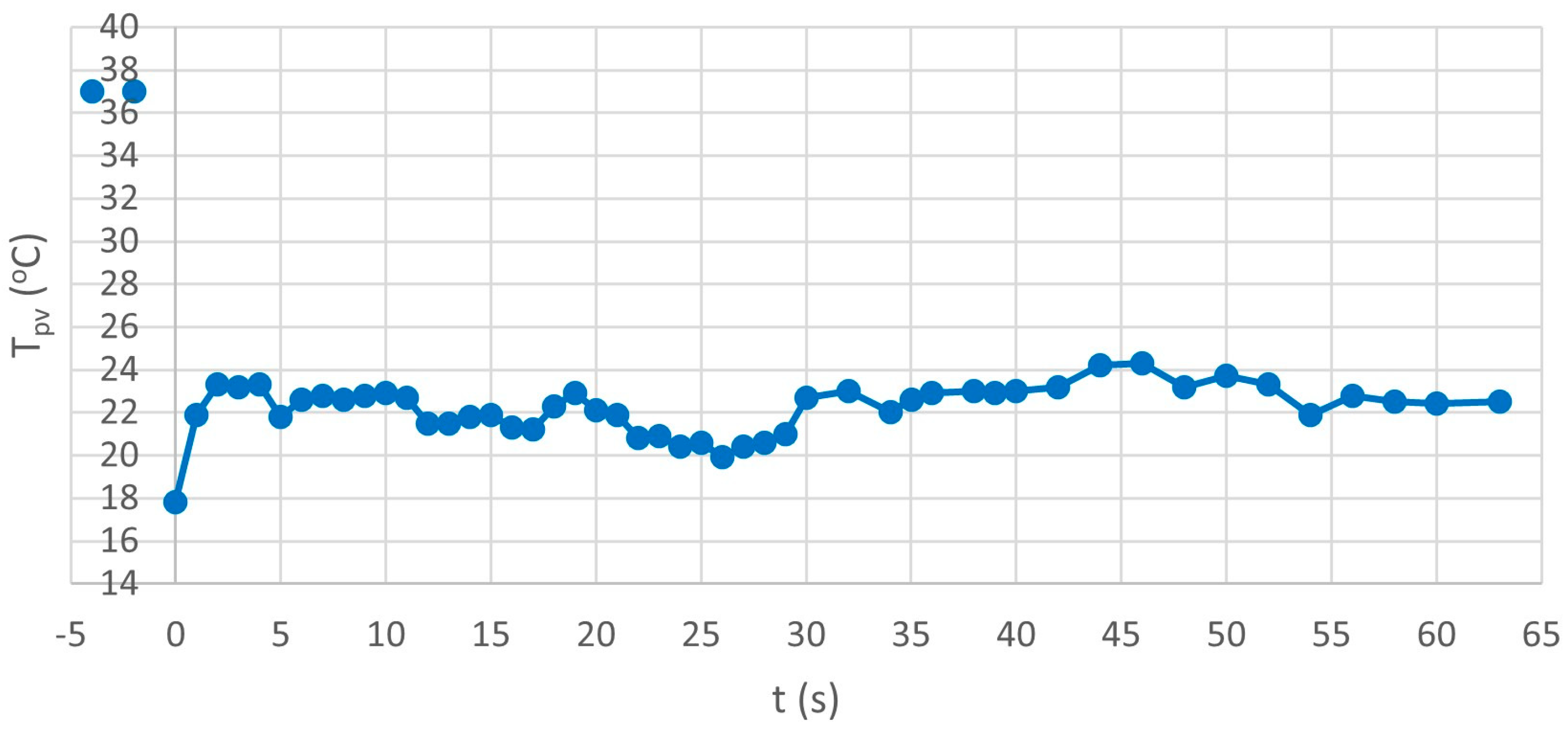
4.1. Experimental T_pv(t) Profiles on the Seashore vs. Inland and Interpretation of the Seawater Splashing Effect

Measured T_pv(t) profiles at the seashore and inland sites are shown in Figure 2 and Figure 3, respectively. Both present the recorded T_pv at steady-state conditions and the transient T_pv(t) profile measured from t = 0, just when the water splashing on the module ends.

Figure 2 shows the T_pv(t) profile of the SW80 module operating on the seashore around solar noon under I_T = 800 W/m², v_w = 0.5–1.0 m/s, T_a = 20 °C, T_s.w. = 15 °C, and RH = 55%, with module inclination β = 35°. The steady-state T_pv was measured 37 °C before s.w. splashing, as shown in Figure 2 for t < 0. Figure 3 shows the measured T_pv(t) profiles as well as the measured T_pv for the SW80 and M55 modules (45 °C and 47 °C, respectively) on a terrace inland under the same I_T and v_w as above, T_a = 21 °C and RH = 45%. The T_pv of the SW80 was 8 °C (45–37 °C), i.e., 18%, lower on the seashore vs. inland (see Figure 2 and Figure 3). This is in agreement with the results reported in [41,45]. The 8 °C difference is attributed mainly to the effect of hu on the seashore and is confirmed in Section 4.3.

Equations (2a,b) and (3) may predict T_pv for inland, and since the measured RH was 45%, there is no need for the hu correction. For the above experimental conditions, the predicted T_pv = T_a + f·I_T = 21 + 0.031·800 = 45.8 °C, which is in good agreement with the measured T_pv = 45 °C for the SW80 module (T_pv,inl−2 curve in Figure 3).

In Figure 3, the steady-state T_pv of the two modules shows 2 °C difference which is due to the difference in their η_pv. This can be derived by theoretically combining Equation (1) and the simplified form f = (1 − η_pv)/U_pv,inl which gives Equation (31).

δT_pv = δf·I_T = −(δη_pv/U_pv,inl)·I_T

(31)

Introducing Equation (31), U_pv,inl = 23 W/m²K [48], I_T = 800 W/m², and the values of η_pv (9.5% and 14.6% for the M55 and SW80, respectively) give δT_pv = 1.8 °C ≈ 2 °C, which is the T_pv difference between the two curves in Figure 3.

For the s.w. volume flow rate per unit width Q/b = 50 mL/s/m, the Δx_o = 0.32 mm, as estimated in Section 3.2.1. When s.w. stopped flowing, Δx(t) decreased (Figure 1). The T_pv(t) profiles in Figure 2 and Figure 3 at t = 0 show a sudden drop due to s.w. splashing on the module, with T_s.w. = 15 °C. For 0 < t < 1 s, phase 1 (see Figure 2), the phenomenon may be approximated by Equation (19). From the experimental data in the seashore environment, the steady-state T_pv = T_f = 37 °C and T_s.w.(t = 0) = 15 °C. Using k_gl = 1 W/mK and k_s.w. = 0.6 W/mK, Equation (19) gives T_f = 28.75 °C on the seashore which is in very good agreement with the measured minimum T_f = 29 °C (see Figure 2). The temperature drop is 8 °C or 22%. Similarly, T_f drops to 35 °C and 37 °C for the SW80 and M55, respectively (Figure 3). In this case, Equation (19) predicts T_f = 33.75 °C and 35 °C, respectively, which are in good agreement with the measured data.

During t = 1–10 s, phase 2 (see Figure 2), Δx thins fast according to Equation (15). At t = 2 s, Δx = 0.116 mm, and at t = 10 s, Δx = 0.056 mm, whereas τ_s.w. < 10 s. T_pv(t) increases fast following 29 °C (1−exp(−t/τ_s.w.)) as the heat exchange due to convection starts prevailing. The increasing T_pv(t) profile (see Section 3.3) may not reach the steady-state T_pv because as T_pv(t) increases, the s.w. evaporation on the module acts as an additional cooling mode. During phase 2, T_pv(t) is 3–5 °C lower than T_pv for about 15–20 s, as shown in Figure 2 and Figure 3.

T_pv(t) in Figure 4 was obtained under the same conditions as the profile in Figure 2. In this case, a lower flow rate Q/b = 40 mL/s/m results in a thinner s.w. layer, as described by Equation (13). In Figure 4, T_pv(t) shows a steep initial drop to 29 °C and then increases fast due to smaller τ_s.w. In phase 2, the T_pv(t) profile is higher than the profile in Figure 2 but shorter due to the lower Q/b and to the s.w. evaporation on the module which has an earlier onset (see Figure 2 and Figure 4). Then, T_pv(t) decreases, during phase 3, following the same profile as the curve in Figure 2.

A higher flow rate, Q/b = 75 mL/s/m split in 3 s.w. shots of 25 mL/s/m every 2 s, led to a T_pv drop of 19.2 °C, as shown in Figure 5. Applying Equation (19) three times, starting with T_pv = 37 °C and T_s.w. = 15 °C, allows the s.w. layer’s temperature to be theoretically determined at the end of each shot. In the third iteration, T_pv(t = 0) is determined equal to 20.4 °C, which is close to the experimental value of 17.8 °C (see Figure 5). The latter has a 52% decrease from the steady-state value of 37 °C. Then, T_pv(t) increases as outlined above during phase 2, and when it reaches 23 °C, it starts decreasing during phase 3 because the evaporation of the s.w. layer on the module prevails. In Figure 5, the rate of s.w. evaporation on the module, m_ev, is smaller because T_pv(t) is lower than in Figure 2 and Figure 4. The three cases presented in Figure 2, Figure 4, and Figure 5 are shown together for comparison in Figure 6.

In Figure 2, Figure 3, Figure 4 and Figure 5 and for around 10–15 s (phase 2), T_pv(t) increases but stays lower than the steady-state value due to s.w. layer evaporation. Thereafter, a significant T_pv(t) decrease appears because the s.w. layer evaporation prevails in phase 3. Specifically, for the case of Q/b = 75 mL/s/m, the T_pv(t) during phase 3 sustains an average value of 22 °C for more than 60 s. This is a 15 °C drop from the steady-state value measured on the seashore and corresponds to a 40% decrease (Figure 5). Compared to the steady-state T_pv measured inland (45 °C), this corresponds to a 51% decrease. On the other hand, for Q/b = 40–50 mL/s/m (Figure 2 and Figure 4), the average decrease in T_pv(t) from its steady-state T_pv value on the seashore, during phase 3, was about 20% and was sustained for 60 s (Figure 6) until the s.w. film evaporated. Compared to the steady-state T_pv measured inland (45 °C), this decrease corresponds to about 35%. Then, T_pv starts increasing during phase 4, following the function (1 − exp(−t/τ)) with a higher time constant, τ = 2 min, according to Equation (18).

4.2. Seawater Evaporation from the PV Module and Its Effect on T_pv

Figure 7 shows the T_pv(t) of the M55 at the inland site after s.w. splashing on the module. The steady-state T_pv = 42 °C underwent a steep drop by 12 °C after s.w. splashing with T_s.w. = 14 °C and under T_a = 17 °C, RH = 45% and v_w = 2 m/s. Equation (19) predicts that T_pv drops initially by 10.6 °C, which is close to the experimental drop (Figure 7). T_pv(t) increases fast during phase 2 and then decreases to around 30 °C during phase 3. This is a 29% decrease from its T_pv value and remains at this lower temperature for 100 s until the water layer entirely evaporates, as theoretically confirmed below. Finally, T_pv increases towards the steady-state T_pv in 5τ, which is in total t = 5 × 2 min = 600 s.

The Mollier diagrams for the above conditions and for T_s.w. = 32 °C during phase 3 give hu_s = 0.032 g s.w./g dry air and hu = 0.0059 g s.w./g dry air. Then, Equation (26) for v_w = 2 m/s gives m_ev/A_pv = 0.45675 g/m²s and Equation (27) gives q = 1071.1 W/m², while Equation (28) for (mc) = 3000 J/m²K for the PV module gives δT_pv/δt = 0.357 °C/s. In Figure 7, T_pv(t = 10) = 35 °C and T_pv(t = 30) = 30 °C. Hence, the time for the temperature to decrease from 35 °C to 30 °C is estimated 5 °C/0.357 °C/s = 14 s. Therefore, T_pv(t) reaches its lower value during phase 3 in 10 + 14 = 24 s compared to the experimental 30 s in Figure 7.

The time period for the s.w. layer Δx(t = 10) to evaporate equals δt_ev = Δx(t = 10)/(m_ev/A_pv). Section 3.2 gives Δx(t = 10) = 0.043 mm and, hence, δt_ev = 94 s. Therefore, the time needed for the s.w. layer to evaporate is equal to 10 s + 94 s = 104 s which is confirmed in Figure 7.

The T_pv,inl-2(t) in Figure 3 shows that in phase 3, the average T_pv(t) = 42 °C while T_a = 21 °C. The Mollier diagrams give hu_s = 0.051 and hu = 0.0059 g s.w./g dry air. Equation (26) gives m_ev/A_pv = 0.56 g/m²s and δt_ev = 57 s. Considering that the start of phase 3 is at 10 s, where T_pv = 42 °C, then the end of phase 3 is estimated at 10 s + 57 s = 67 s, compared to around 60 s in the experimentally identified phase 3 in Figure 3.

4.3. Steady-State T_pv Prediction by the Proposed Model Taking into Account RH, T_a, T_s.w.

Equations (1)–(9) predict T_pv provided the difference in the heat convection coefficient for RH = 55% with reference to RH = 45% being estimated (Equation (7b)). The air flow in the experimental conditions was laminar forced flow. Substituting into Equation (5), the ν_α, ν_s.w., Pr_a, Pr_s.w., k_a, and k_s.w. values corresponding to T_a and T_s.w. give h_c,s.w. = 195h_c,a. The Mollier diagrams for the SW80 on the seashore (RH = 55% and T_a = 20 °C) and inland site (RH = 45% and T_a = 21 °C) give the % concentration in g-mol of both H₂O and dry air. Specifically,

• The relative concentration is 0.98565% g-mol dry air and 0.014345% g-mol H₂O in the humid air at RH_s.e. = 55%.
• The relative concentration is, correspondingly, 0.9885% g-mol dry air and 0.01147% g-mol H₂O in the humid air at RH_inl = 45%.

At saturated air, T_a = T_s.w. and hu_s = 0.014659 g H₂O/g dry air or 17.3 g H₂O/m³ air.

The heat convection coefficient h_c,a is estimated to be 20 W/m²K, and Equation (7a) for laminar forced flow gives h_c,55% = 75.6 W/m²K and h_c,45% = 64.6 W/m²K.

Therefore, δh_c,hu = 11.0 W/m²K and U_pv,s.e. = U_pv,inl + δh_c,hu = 34 W/m²K. The hu correction term in Equation (9) (1−δh_c,hu/U_pv,s.e.) = 0.676. Equation (8), for f_inl = 0.031, gives f_s.e.= 0.031·0.676 = 0.021 and T_pv = T_a + f_s.e.·I_T = 20 °C + 0.021 m²K/W·800 W/m² = 36.8 °C, which is 0.5% lower than the measured value of 37 °C, in Figure 2.

Considering Equation (1), the error in the estimation of T_pv is the error in the measurement of T_a = ±0.5 °C (see Section 2), plus the error in the measurement in I_T which is negligible (see Section 2) times f, plus I_T times the error in the estimation of f. The latter was estimated in the third decimal digit. Hence, the error in the estimation of f·I_T is ±(0.001 m²K/W)·800 W/m² = ±0.8 °C. Therefore, the total error in the prediction of T_pv is ±1.3 °C while the accuracy in the T_pv measurement was ±1 °C. Similarly, in the prediction of T_pv using Equations (1)–(9), the analysis gives an additional contribution to the error due to the estimation of δh_c,hu/U_pv, which is equal to 3%, and that corresponds to an additional error in T_pv of ±0.7 °C. Therefore, the overall error in the estimation in T_pv accounting for the hu sums up to ±2 °C, which is an acceptable range in the estimation of T_pv.

4.4. Comparison with Other T_pv Prediction Models

Considering the experimental conditions on the seashore site, T_a = 20 °C, I_T = 800 W/m², v_w = 1 m/s, and RH = 55%, the measured T_pv =37 °C at the steady-state is compared to the predicted T_pv by the model proposed in this study, Equations (1)–(9), and to other existing models for FPV systems, Equations (32)–(38), in

Table 1. Predicted T_pv using the proposed model compared with other existing models for the s.e.

Ref.	Model	Equation	Tpv Predicted (°C)
	Proposed model: Equations (1)–(9)		36.8
[43]	Tpv = 26.97 + 0.77Ta + 0.023IT − 0.206RH −0.137vw	(32)	49.3
[15]	Tpv = 0.961Ta + 0.029IT − 1.457vw + 0.000(°C/degree direction) + 0.109RH + 1.57 °C	(33)	48.5
[15]	Tpv = 0.942Ta + 0.028IT − 1.509vw + 3.9 °C	(34)	43.6
[16]	Tpv = 0.9458Ta + 0.0215IT − 1.2376vw + 2.0458	(35)	36.9
[16]	Tpv = 0.9282Ta + 0.021IT − 1.221vw + 0.0246Tw + 1.8081	(36)	36.3
[48]	Tpv = [TaUf + TwUb + ((τα) −ηref − γηrefTref)IT]/(Uf + Ub − γηrefIT)	(37)	39.1
[14]	Tpv = Ta + 0.32 IT/(8.91 + 2.0vw)	(38)	43.5

.

In Equation (37), (τα) = 0.9 is the effective transmission–absorption coefficient of the PV module with η_ref = 0.146 at STC. The values used for the heat losses coefficients U_f and U_b are 18.355 and 10.209 W/m²K, respectively, as proposed in [48].

This comparative analysis for the T_pv prediction by the proposed model and the seven other formulas in Table 1 confirms that the approach outlined in this paper, taking into account the RH and the T_s.w., gives results closer to those measured in the s.e. Apart from Equations (35) and (36), [16], which gave very good prediction results, the other T_pv prediction formulas overestimated T_pv.

5. Discussion

The recuperation in η_pv due to enhanced natural cooling is estimated at 4% by introducing in Equation (30) two steady-state T_pv values: 37 °C (Figure 5) on the seashore and 45 °C (T_pv,inl-2, Figure 3) inland. This recuperation in η_pv is attributed to the higher humidity in the s.e. with the module operating at SOC. Comparing the average T_pv(t) = 22 °C during phase 3 on the seashore with the steady-state T_pv = 45 °C inland leads to a 11.5% recuperation due to the combined effect of the humidity as well as the seawater cooling and evaporation on the modules. Similar efficiency gains are anticipated for FPV operation in freshwater environments due to the higher humidity present in the vicinity of lakes and reservoirs and the water evaporation on the modules.

While low wind speed conditions were present during the experiments on the seashore and inland, it is expected that higher wind speeds, which usually prevail in the s.e., would lead to a much higher efficiency recuperation for FPV. A higher v_w = 4 m/s in Equation (3) leads to an overall f_s.e. = 0.0136 m²K/W accounting for the effect of the higher wind speed and humidity and, therefore, T_pv= T_a + f_s.e.·I_T = 20 °C + 0.0136 m²K/W·800 W/m² = 30.9 °C. This additional decrease in T_pv by 6.1 °C, accounting for the effect of wind, with v_w = 4 m/s, would lead to a total recuperation of 7% at steady-state and 14.5% when s.w. splashing and evaporation on the modules are also considered.

While the aforementioned efficiency gains are significant, some losses may be encountered due to a thin layer of salt that remains after the s.w. layer evaporation on the PV module, which may lead to a reduction in the solar irradiance reaching the PV cells [60]. Long-term exposure to humid and saline environments can lead to corrosion, potential-induced degradation (PID), and other PV degradation effects reducing the module and system lifetime [19,21,60,61]. Biofouling effects, including algae growth on PV modules, may pose additional challenges [62,63]. The application of nanocoatings with self-cleaning and anti-fouling properties on PV glass [64], the use of anticorrosive PV material [63], and improved multilayer backsheets [61], as well as frequent cleaning, may mitigate some of these risks. Considering energy yield gains between 5 and 10% in FPV, a 3–9% higher LCOE is estimated for FPV systems in freshwater environments compared to LBPV in [65]. While FPV platforms at the s.e. are at the early stages of development, it is anticipated that the estimated efficiency recuperation due to higher humidity and s.w. cooling and evaporation on the PV modules may partially counterbalance the higher CAPEX costs. A full investigation into all the aforementioned effects would be needed for long-term performance predictions and estimation of the levelized cost of electricity for FPV operating at the s.e., which is outside the scope of the present article.

6. Conclusions

The PV cooling of c-Si modules operating on the seashore and inland sites was theoretically and experimentally studied through steady-state and transient temperature profiles. The research covered seawater splashing on the modules and the subsequent seawater layer evaporation as well as the effect of humidity. An improved model for the prediction of steady-state T_pv incorporating the effect of humidity is proposed, and complete theoretical analysis of the PV cooling phenomena after seawater splashing and the subsequent evaporation of the seawater layer from the module is provided. The T_pv prediction results were compared to measured values both inland and on the seashore, simulating FPV conditions, and were shown to be in very good agreement.

The research analysis showed that the T_pv profiles of the front side depend on the pattern of the seawater flow on the PV and the environmental conditions, including the humidity. Specifically:

• T_pv depends on the humidity and decreases as hu increases from low to medium values in a clear sky. For relative humidity 55% on the seashore compared to 45% inland, the steady-state T_pv was both predicted and measured about 18% lower on the seashore. This corresponds to a 4% higher efficiency on the seashore compared to inland, which is mainly attributed to the difference in humidity as v_w, I_T, and T_a were almost the same on the seashore and inland sites.
• The transient T_pv(t) profile depends on the pattern of seawater splashing on the module. After seawater splashing, a steep temperature drop of 22% lasting for 2 s was measured and theoretically confirmed. The drop depends on the seawater temperature and the mode it splashes on the modules. This reached 52% when the pattern of the s.w. flow on the module was three shots of 25 mL/s per unit width of the module.
• T_pv is affected by the subsequent seawater layer evaporation on the module which caused an overall decrease between 20 and 40% (depending on the flow pattern) compared to the steady-state value on the seashore before the seawater splash. This decrease lasted for 60–100 s, depending on the seawater flow rate and mode of splashing, which was theoretically predicted and experimentally confirmed.
• The T_pv profiles on the seashore with seawater splashing on the modules were 35–51% lower compared to the steady-state inland values.
• Taking into consideration the effect of humidity as well as the seawater cooling and evaporation on the modules, it was estimated that the PV efficiency on the seashore was 11.5% higher than inland.

This research disclosed the importance of the effect of humidity on PV temperature as well as the effect of the seawater splashing and its evaporation on the modules, whose combined effect leads to significant recuperation in the operating efficiency on the seashore compared to inland. While low wind speed conditions were present during the experiments, it is expected that higher wind speeds, which are usual in the sea environment, would lead to the recuperation of much higher efficiency for FPV.

References

1. Vats, K.; Tiwari, G.N. Performance evaluation of a building integrated semitransparent photovoltaic thermal system for roof and façade. Energy Build. 2012, 45, 211–218. [Google Scholar] [CrossRef]
2. Ghosh, A.; Sarmah, N.; Sundaram, S.; Mallick, T.K. Numerical studies of thermal comfort for semi-transparent building integrated photovoltaic (BIPV)-vacuum glazing system. Sol. Energy 2019, 190, 608–616. [Google Scholar] [CrossRef]
3. Assoa, Y.B.; Gaillard, L.; Menezo, C.; Negri, N.; Sauzedde, F. Dynamic prediction of a building integrated photovoltaic system thermal behaviour. Appl. Energy 2018, 214, 73–82. [Google Scholar] [CrossRef]
4. Kaplanis, S.; Kaplani, E. A New Dynamic Model to Predict Transient and Steady State PV Temperatures Taking into Account the Environmental Conditions. Energies 2019, 12, 2. [Google Scholar] [CrossRef] [Green Version]
5. Kaldellis, J.; Kapsali, M.; Kavadias, K. Temperature and wind speed impact on the efficiency of PV installations. Experience obtained from outdoor measurements in Greece. Renew. Energy 2014, 66, 612–624. [Google Scholar] [CrossRef]
6. Lobera, D.T.; Valkealahti, S. Dynamic thermal model of solar PV systems under varying climatic conditions. Sol. Energy 2013, 93, 183–194. [Google Scholar] [CrossRef]
7. Luketa-Hanlin, A.; Stein, J.S. Improvement and Validation of a Transient Model to Predict Photovoltaic Module Temperature; Sandia National Laboratories: Albuquerque, NM, USA, 2012.
8. Kaplani, E.; Kaplanis, S. Thermal modelling and experimental assessment of the dependence of PV module temperature on wind velocity and direction, module orientation and inclination. Sol. Energy 2014, 107, 443–460. [Google Scholar] [CrossRef] [Green Version]
9. Kaplani, E.; Kaplanis, S. Dynamic Electro-Thermal PV Temperature and Power Output Prediction Model for Any PV Geometries in Free-Standing and BIPV Systems Operating under Any Environmental Conditions. Energies 2020, 13, 4743. [Google Scholar] [CrossRef]
10. Kaplanis, S.; Kaplani, E.; Kaldellis, J.K. PV temperature and performance prediction in free-standing, BIPV and BAPV incorporating the effect of temperature and inclination on the heat transfer coefficients and the impact of wind, efficiency and ageing. Renew. Energy 2022, 181, 235–249. [Google Scholar] [CrossRef]
11. Faiman, D. Assessing the outdoor operating temperature of photovoltaic modules. Prog. Photovolt. Res. Appl. 2008, 16, 307–315. [Google Scholar] [CrossRef]
12. Ciulla, G.; Lo Brano, V.; Moreci, E. Forecasting the cell temperature of PV modules with an adaptive system. Int. J. Photoenergy 2013, 2013, 192854. [Google Scholar] [CrossRef]
13. Schwingshackl, C.; Petitta, M.; Wagner, J.E.; Belluardo, G. Wind effect on PV module temperature: Analysis of different techniques for an accurate estimation. Energy Procedia 2013, 40, 77–86. [Google Scholar] [CrossRef] [Green Version]
14. Skoplaki, E.; Boudouvis, A.G.; Palyvos, J.A. A simple correlation for the operating temperature of photovoltaic modules of arbitrary mounting. Sol. Energy Mater. Sol. Cells 2008, 92, 1393–1402. [Google Scholar] [CrossRef]
15. TamizhMani, G.; Ji, L.; Tang, Y.; Petacci, L.; Osterwald, C. Photovoltaic module thermal/wind performance: Long term monitoring and model development for energy rating. In Proceedings of the NCPV and Solar Program Review Meeting Proceedings, Denver, CO, USA, 24–26 March 2003; pp. 936–939. [Google Scholar]
16. Kamuyu, W.C.L.; Lim, J.R.; Won, C.S. Prediction model of Photovoltaic Module Temperature for Power Performance of Floating PVs. Energies 2018, 11, 447. [Google Scholar] [CrossRef] [Green Version]
17. Graditi, G.; Ferlito, S.; Adinolfi, G.; Tina, G.M.; Ventura, C. Energy yield estimation of thin-film photovoltaic plants by using physical approach and artificial neural networks. Solar Energy 2016, 130, 232–243. [Google Scholar] [CrossRef]
18. Dubey, S.; Sarvaiya, J.N.; Seshadri, B. Temperature dependent photovoltaic (PV) efficiency and its effect on PV production in the world—A review. Energy Procedia 2013, 33, 311–321. [Google Scholar] [CrossRef] [Green Version]
19. Hacke, P.; Spataru, S.; Terwilliger, K.; Perrin, G.; Glick, S.; Kurtz, S.; Wohlgemuth, J. Accelerated testing and modeling of potential-induced degradation as a function of temperature and relative humidity. IEEE J. Photovolt. 2015, 5, 1549–1553. [Google Scholar] [CrossRef]
20. Kempe, M.D.; Wohlgemuth, J.H. Evaluation of temperature and humidity on PV module component degradation. In Proceedings of the IEEE 39th Photovoltaic Specialists Conference (PVSC), Tampa, FL, USA, 16–21 June 2013; pp. 0120–0125. [Google Scholar] [CrossRef]
21. Park, N.C.; Oh, W.W.; Kim, D.H. Effect of Temperature and Humidity on the Degradation Rate of Multicrystalline Silicon Photovoltaic Module. Int. J. Photoenergy 2013, 2013, 925280. [Google Scholar] [CrossRef] [Green Version]
22. Kaplanis, S.; Kaplani, E.; Borza, P.N. PV defects identification through a synergistic set of non-destructive testing (NDT) techniques. Sensors 2023, 23, 3016. [Google Scholar] [CrossRef]
23. Cazzaniga, R.; Rosa-Clot, M. The booming of floating PV. Sol. Energy 2021, 219, 3–10. [Google Scholar] [CrossRef]
24. Rosa-Clot, M.; Tina, G.M.; Nizetic, S. Floating photovoltaic plants and wastewater basins: An Australian project. Energy Procedia 2017, 134, 664–674. [Google Scholar] [CrossRef]
25. Tina, G.M.; Scavo, F.B.; Merlo, L.; Bizzarri, F. Comparative analysis of monofacial and bifacial photovoltaic modules for floating power plants. Appl. Energy 2021, 281, 116084. [Google Scholar] [CrossRef]
26. Sahu, A.; Yadav, N.; Sudhakar, K. Floating photovoltaic power plant: A review. Renew. Sustain. Energy Rev. 2016, 66, 815–824. [Google Scholar] [CrossRef]
27. Wild, M.; Folini, D.; Hakuba, M.Z.; Schär, C.; Seneviratne, S.I.; Kato, S.; Rutan, D.; Ammann, C.; Wood, E.F.; König-Langlo, G. The energy balance over land and oceans: An assessment based on direct observations and CMIP5 climate models. Clim. Dyn. 2015, 44, 3393–3429. [Google Scholar] [CrossRef] [Green Version]
28. Lindfors, A.V.; Hertsberg, A.; Riihela, A.; Carlund, T.; Trentmann, J.; Mueller, R. On the Land-Sea Contrast in the Surface Solar Radiation (SSR) in the Baltic Region. Remote Sens. 2020, 12, 3509. [Google Scholar] [CrossRef]
29. Govardhanan, M.S.; Kumaraguruparan, G.; Kameswari, M.; Saravanan, R.; Vivar, M.; Srithar, K. Photovoltaic Module with Uniform Water Flow on Top Surface. Int. J. Photoenergy 2020, 2020, 8473253. [Google Scholar] [CrossRef]
30. Kerzika, A.H.; Barimah, B.; Aurelien, K.K.C. Photovoltaic Solar Panel Cooled with Runoff Water. Int. J. Energy Eng. 2020, 10, 41–45. [Google Scholar]
31. Sukarno, K.; Hamid, A.S.A.; Razali, H.; Dayou, J. Evaluation on cooling effect on solar PV power output using Laminar H2O surface method. Int. J. Renew. Energy Res. 2017, 7, 1213–1217. [Google Scholar]
32. Iqbal, S.; Afzal, S.; Mazhar, A.U.; Anjum, H.; Diyyan, A. Effect of Water Cooling on the Energy Conversion Efficiency of PV Cell. Am. Sci. Res. J. Eng. Technol. Sci. 2016, 20, 122–128. [Google Scholar]
33. Nižetić, S.; Čoko, D.; Yadav, A.; Grubišić-Čabo, F. Water spray cooling technique applied on a photovoltaic panel: The performance response. Energy Convers. Manag. 2016, 108, 287–296. [Google Scholar] [CrossRef]
34. Bahaidarah, H.M.S. Experimental performance evaluation and modelling of jet impingement cooling for thermal management of photovoltaics. Sol. Energy 2016, 135, 605–617. [Google Scholar] [CrossRef]
35. Bahaidarah, H.; Subhan, A.; Gandhidasan, P.; Rehman, S. Performance evaluation of a PV (photovoltaic) module by back surface water cooling for hot climatic conditions. Energy 2013, 59, 445–453. [Google Scholar] [CrossRef]
36. Chandrasekhar, M.; Suresh, S.; Senthilkumar, T.; Karthikeyan, M.G. Passive cooling of standalone flat PV module with cotton wick structures. Energy Convers. Manag. 2013, 71, 43–50. [Google Scholar] [CrossRef]
37. Alami, A.H. Effects of evaporative cooling on efficiency of photovoltaic modules. Energy Convers. Manag. 2014, 77, 668–679. [Google Scholar] [CrossRef]
38. Kumar, M.; Niyaz, H.M.; Gupta, R. Challenges and opportunities towards the development of floating photovoltaic systems. Sol. Energy Mater. Sol. Cells 2021, 233, 111408. [Google Scholar] [CrossRef]
39. Trapani, K.; Millar, D.L. The thin film flexible floating PV (T3F-PV) array: The concept and development of the prototype. Renew. Energy 2014, 71, 43–50. [Google Scholar] [CrossRef]
40. Liu, L.; Wang, Q.; Lin, H.; Li, H.; Sun, Q.; Wennersten, R. Power Generation Efficiency and Prospects of Floating Photovoltaic Systems. Energy Procedia 2017, 105, 1136–1142. [Google Scholar] [CrossRef]
41. Dorenkamper, M.; Wahed, A.; Kumar, A.; de Jong, M.; Kroon, J.; Reindl, T. The cooling effect of floating PV in two different climate zones: A comparison of field test data from the Netherlands and Singapore. Sol. Energy 2021, 219, 15–23. [Google Scholar] [CrossRef]
42. Bonkaney, A.L.; Madougou, S.; Adamou, R. Impact of Climatic Parameters on the Performance of Solar Photovoltaic (PV) Module in Niamey. Smart Grid Renew. Energy 2017, 8, 379–393. [Google Scholar] [CrossRef] [Green Version]
43. Almaktar, M.; Rahman, H.A.; Hassan, M.Y.; Rahman, S. Climate Based Empirical Model for PV Module Temperature Estimation in Tropical Environment. Appl. Sol. Energy 2013, 49, 192–201. [Google Scholar] [CrossRef]
44. Liu, H.; Krishna, V.; Leung, J.L.; Reindl, T.; Zhao, L. Field experience and performance analysis of floating PV technologies in the tropics. Progr. Photovolt. Res. Appl. 2018, 26, 957–967. [Google Scholar] [CrossRef]
45. Luo, W.; Isukapalli, S.N.; Vinayagam, L.; Ting, S.A.; Pravettoni, M.; Reindl, T.; Kumar, A. Performance loss rates of floating photovoltaic installations in the tropics. Sol. Energy 2021, 219, 58–64. [Google Scholar] [CrossRef]
46. Kjeldstad, T.; Lindholm, D.; Marstein, E.; Selj, J. Cooling of floating photovoltaics and the importance of water temperature. Sol. Energy 2021, 218, 544–551. [Google Scholar] [CrossRef]
47. Lindholm, D.; Kjeldstad, T.; Selj, J.; Marstein, E.S.; Fjær, H.G. Heat loss coefficients computed for floating PV modules. Prog. Photovolt. Res. Appl. 2021, 29, 1262–1273. [Google Scholar] [CrossRef]
48. Niyaz, H.M.; Kumar, M.; Gupta, R. Estimation of module temperature for water-base photovoltaic systems. J. Renew. Sustain. Energy 2021, 13, 053705. [Google Scholar] [CrossRef]
49. Golroodbari, S.Z.; van Sark, W. Simulation of performance differences between offshore and land-based photovoltaic systems. Prog. Photovolt. Res. Appl. 2020, 28, 873–886. [Google Scholar] [CrossRef]
50. Kazem, H.A.; Chaichan, M.T. Effect of humidity on Photovoltaic Performance based on experimental study. Int. J. Appl. Eng. Res. 2015, 10, 43572–43577. [Google Scholar]
51. Chaicham, M.T.; Kazem, H.A. Experimental analysis of solar intensity on photovoltaic in hot and humid weather conditions. Int. J. Sci. Eng. Res. 2016, 7, 91–96. [Google Scholar]
52. Choi, J.H.; Hyun, J.H.; Lee, W.; Bhang, B.-G.; Min, Y.K.; Ahn, H.-K. Power performance of high density photovoltaic module using energy balance model under high humidity environment. Sol. Energy 2021, 219, 50–57. [Google Scholar] [CrossRef]
53. Dirnberger, D.; Blackburn, G.; Müller, B.; Reise, C. On the impact of solar spectral irradiance on the yield of different PV technologies. Sol. Energy Mater. Sol. Cells 2015, 132, 431–442. [Google Scholar] [CrossRef]
54. Tashtoush, B.; Al-Oqool, A. Factorial analysis and experimental study of water-based cooling system effect on the performance of photovoltaic module. Int. J. Environ. Sci. Technol. 2019, 16, 3645–3656. [Google Scholar] [CrossRef]
55. Lienhard, J.H., IV; Lienhard, J.H., V. A Heat Transfer Textbook, 3rd ed.; Phlogiston Press: Cambridge MA, USA, 2003. [Google Scholar]
56. White, F.M. Heat and Mass Transfer; Addison-Wesley Publishing Co.: Boston, MA, USA, 1988. [Google Scholar]
57. Ilha, A.; Doria, M.M.; Aibe, V.Y. Treatment of the Time Dependent Residual Layer and its Effects on the Calibration Procedures of Liquids and Gases Inside a Volume Prover. In Proceedings of the 15th Flow Measurement Conference (FLOMEKO), Taipei, Taiwan, 13–15 October 2010. [Google Scholar]
58. Shah, M.M. Methods for calculation of evaporation from swimming pools and other water surfaces. ASHRAE Trans. 2014, 120 Pt 2, 3–17. [Google Scholar]
59. Mattei, M.; Notton, G.; Cristofari, C.; Muselli, M.; Poggi, P. Calculation of the polycrystalline PV module temperature using a simple method of energy balance. Renew. Energy 2006, 31, 553–567. [Google Scholar] [CrossRef]
60. Mannino, G.; Tina, G.M.; Cacciato, M.; Merlo, L.; Cucuzza, A.V.; Bizzarri, F.; Canino, A. Photovoltaic Module Degradation Forecast Models for Onshore and Offshore Floating Systems. Energies 2023, 16, 2117. [Google Scholar] [CrossRef]
61. Zhang, J.-W.; Cao, D.-K.; Diaham, S.; Zhang, X.; Yin, X.-Q.; Wang, Q. Research on potential induced degradation (PID) of polymeric backsheet in PV modules after salt-mist exposure. Sol. Energy 2019, 188, 475–482. [Google Scholar] [CrossRef]
62. Almeida, R.M.; Schmitt, R.; Grodsky, S.M.; Flecker, A.S.; Gomes, C.P.; Zhao, L.; Liu, H.; Barros, N.; Kelman, R.; McIntyre, P.B. Floating solar power could help fight climate change—Let’s get it right. Nature 2022, 606, 246–249. [Google Scholar] [CrossRef]
63. Wang, J.; Lund, P.D. Review of recent offshore photovoltaics development. Energies 2022, 15, 7462. [Google Scholar] [CrossRef]
64. Arabatzis, I.; Todorova, N.; Fasaki, I.; Tsesmeli, C.; Peppas, A.; Li, W.X.; Zhao, Z. Photocatalytic, self-cleaning, antireflective coating for photovoltaic panels: Characterization and monitoring in real conditions. Sol. Energy 2018, 159, 251–259. [Google Scholar] [CrossRef]
65. World Bank Group; Energy Sector Management Assistance Program; The Solar Energy Research Institute of Singapore. Where Sun Meets Water: Floating Solar Handbook for Practitioners; World Bank: Washington, DC, USA, 2019. [Google Scholar]
Figure 1. Seawater layer thickness Δx vs. t when the flow stopped and the layer started thinning. The flow rate per unit width was 50 mL/s/m on a module inclined at 35° and Ts.w. = 30 °C.
Energies 16 04756 g001
Figure 2. Tpv(t) for the SW80 module on the seashore site. The steady-state Tpv values are shown at t < 0. The Tpv(t) profile begins at t = 0 at the end of the s.w. flow on the module with Q/b = 50 mL/s/m. The regions defined by the red dashed lines represent phase 1, phase 2, and phase 3.
Energies 16 04756 g002
Figure 3. Tpv(t) profile for the M55 (Tpv,inl-1) and the SW80 (Tpv,inl-2) modules measured on the site inland. The steady-state Tpv values are shown at t < 0. The Tpv(t) profile begins at t = 0 at the end of the s.w. flow on the module with Q/b = 50 mL/s/m.
Energies 16 04756 g003
Figure 4. Tpv(t) for the SW80 module on the seashore site. The steady-state Tpv values are shown at t < 0. The Tpv(t) profile begins at t = 0 at the end of the s.w. flow on the module with Q/b = 40 mL/s/m.
Energies 16 04756 g004
Figure 5. Tpv(t) for the SW80 module on the seashore site. The steady-state Tpv values are shown at t < 0. The Tpv(t) profile begins at t = 0 at the end of the s.w. flow on the module with Q/b = 75 mL/s/m split in 3 shots of 25 mL/s/m each.
Energies 16 04756 g005
Figure 6. Comparative presentation of Tpv(t) profiles as in Figure 2, Figure 4, and Figure 5 corresponding to Tpv,s-1, Tpv,s-2, and Tpv,s-3, respectively.
Energies 16 04756 g006
Figure 7. Tpv(t) transient profile of the M55 module operating inland after s.w. splashing of Ts.w. = 14 °C.
Energies 16 04756 g007