Analysis of Wind Farms under Different Yaw Angles and Wind Speeds

Abstract

Wind farm optimization is pivotal in maximizing energy output, reducing costs, and minimizing environmental impact. This study comprehensively explores wind farm behavior under varying wind conditions and yaw angles to achieve these objectives. The primary motivation is to optimize wind farm performance and efficiency through proper yaw adjustment in response to wind speed changes. A computational investigation using a three-by-three wind turbine array was conducted, employing large eddy simulation (LES) to evaluate wind farm performance. Nine LES cases were considered, incorporating three wind speeds (7.3 ms⁻¹, 10.4 ms⁻¹, and 4.3 ms⁻¹) and three yaw angles (30°, 20°, and 0°), with nearly constant turbulence intensity (TI) at 12.0%. The impact of wind speed and yaw angles on wake characteristics and power outputs were analyzed. The findings reveal that wind speed has limited influence on wake characteristics and power outputs, except for lower wind speeds at a yaw angle of 20 degrees. These results contribute to understanding wind farm performance optimization, aiding in developing strategies to enhance energy extraction while minimizing costs and environmental implications.

1. Introduction

With more initiatives worldwide towards greener energy to mitigate climate change, wind energy has been a leading source. The Intergovernmental Panel on Climate Change (IPCC) special report 15 [1] stated that renewable energy needs to increase from 20% in 2018 to 67% in 2050 to limit global temperature rise to 1.5 °C. More wind farms are being built onshore and offshore to reach that goal. However, proper optimization (i.e., design, operation, control, and grid integration) is still a concern under different conditions of wind farms and the turbulent atmospheric boundary layer (ABL). This is due to the complex interactions between the wind farms and the ABL, whose flow properties are greatly affected by surface roughness, thermal effects, different forcing parameters, among others.

In a wind farm, upstream turbines affect the downstream ones as they extract energy from the upcoming wind while enhancing the turbulence levels and reducing the wind speed in the flow. This phenomenon is known as the wake effect or wake loss, and it can cause a decrease in the overall power output of the wind farm. There are several ways to improve the annual energy production (AEP) of a wind farm, such as pitch and torque control, layout optimization, tilt, and yaw misalignment of wind turbines [2,3,4]. Wake steering becomes essential, especially when turbines are placed closely, since sparse installations increase costs, particularly cabling. In wake steering, by trading off the power of the upstream turbines, a higher net power of a wind farm is achieved. Wake steering also reduces the fluctuation of wind energy, improving its reliability within the larger power grid. Prior studies [2,3,4,5] have demonstrated that the degree of wake deflection increases as the flow travels further downstream. The amount of deflection is dictated by the yaw misalignment, the wind speed and direction, the incoming turbulence level, the thermal stability, the thrust coefficient, and other factors (i.e., turbine parameters, surface roughness).

Inflow conditions such as wind speeds, turbulence intensity, and yaw angles affect the flow properties inside the wind farm, thus influencing the power output and the flow-induced dynamic loads of every turbine [6]. Furthermore, the unsteady oscillations of the wake (also known as wake meandering) by eddies larger than the turbine diameter also have important implications for the performance and reliability of wind turbines in a wind farm [7,8]. Under the influences of the different environmental conditions, the turbines experience leading-edge erosion; this affects the aerodynamics and AEP of the wind farm [9,10]. Understanding turbine wake aerodynamics in diverse incoming flow conditions is crucial to enhancing wind farm design, maximizing power output, and minimizing maintenance costs. Several methods are available, including analytical modeling, computational fluid dynamics (CFD), wind-tunnel experiments, and field experiments to study the multi-scale interactions between wind turbines and the atmospheric boundary layer. The experimental and numerical studies [11,12,13] of single-turbine wakes have shown that the velocity deficit profiles usually have a two-dimensional axisymmetric Gaussian distribution maximum located at hub height in the near wake region. This characteristic of the velocity deficit profiles augments the turbulent mixing of the incoming flow and the wake. When a wind turbine experiences yawed conditions, counter-rotating vortices form in the turbine’s wake, which can interact with the atmospheric boundary layer and cause the wake to take on a kidney shape [14]. The velocity and turbulence levels distribution are thus impacted by the yaw misalignments in all directions [15,16]. The wake characteristics of a yawed flow have been studied using various theoretical and computational models, such as mass and momentum conservation [5], Reynolds-averaged Navier–Stokes (RANS) equations with vortex theory [16], and others [17,18].

As the wake moves downstream, it undergoes several changes. One of these changes is the growth of the wake in both lateral and vertical directions, which is due to the entrainment of the outer flow. Another change in the wake as it moves downstream is the increase in the value of the streamwise velocity component until it eventually recovers to the same value as the surrounding flow [19]. Several studies [6,20,21] have shown that the turbulence intensity level strongly influences the wake recovery rate in the incoming flow. Elevated turbulence levels in the incoming flow lead to better mixing of the wake region with the atmospheric boundary layer. This momentum exchange helps the breakdown of large vortices into smaller ones leading to a faster wake recovery [22]. Higher turbulence levels expedite the faster wake recovery, thus affecting the performances of downstream turbines in wind farms.

When wind flows through a wind turbine, it experiences a change in velocity and pressure as it passes over the rotor blades. This phenomenon causes the wind to separate into layers: the wake region behind the turbine and the atmospheric boundary layer above it. Slower wind speeds and higher turbulence characterize the wake region, where most of the energy extraction occurs. As the wake region moves downstream, it mixes with the surrounding atmospheric layer and creates a shear layer with a significant velocity gradient. Due to the non-uniform logarithmic velocity profile, a non-axisymmetric shear layer is formed, particularly pronounced at the top edge of the turbine. As a result, there is a higher production of turbulent kinetic energy at the upper edge of the wake, leading to an amplification of turbulence levels in that region [12,13,23,24,25,26]. The turbulence intensity in the wake zone typically has a double Gaussian profile with two peaks at the edges of the wake [20,27]. The transition between near-wake and far-wake occurs from the maxima of the turbulence levels forward, and then turbulence intensity decreases monotonically with downstream distance.

Numerous variables, such as the unpredictability of the local wind speed and the transport properties of turbulence in the wake, affect the best turbine configuration in every wind farm architecture. The biggest factor contributing to the decline in wind farm efficiency is variability in wind speed [28]. After accurately assessing the wind speed variations by appropriate methods (for more details, see [29,30,31,32]), their subsequent effects on the aerodynamic characteristics need to be studied. The wake characteristics under high wind speeds while estimating the wind conditions by proper model [33] are also very crucial. How the turbulent wake flow structures within the wind farms under full-wake and partial-wake conditions affect the power output under different wind speeds and yaw angles is underexplored. Most studies [4,34] investigated the performance of wind farms just by changing the layout or yaw angles on a single wind speed mainly by reduced-order models. They found that layout and wake steering are complementary to maximize AEP and minimize wake losses. Field studies are not entirely conclusive when the wake steering effects on the performance of wind turbines are analyzed [35,36]. There have been some studies [37,38] on the effects of steering at variable wind speeds with a few turbines in a row. Howland et al. [37] showed improved power maximization with a row of six turbines at a fixed yaw angle of 20°. Simley et al. [38] found the effectiveness of wake steering in improving energy production was observed for wind speeds ranging from 4–12 m/s with two turbines, except for 6–8 m/s due to higher wind direction variability and power loss from yaw misalignment, while its efficacy for wind speeds between 12–14 m/s remains uncertain due to insufficient data.

To the authors’ knowledge, no rigorous studies have been conducted on the combined effect of yaw angle and wind speed on the wind farm’s performance and wake physics. Since the performance of wind farms can be significantly affected by the yaw angle and wind speed, understanding these effects is crucial for designing and operating wind farms effectively. Therefore, finding the optimal combination of yaw angle and wind speed is crucial for maximizing wind farms’ power output and efficiency. The paper is structured as follows: Section 2 comprehensively explains the numerical details employed in the study. In Section 3, the wind farm flow statistics are presented and thoroughly discussed. Finally, Section 4 offers a concise summary of the entire analysis.

2. Numerical Methods

2.1. Governing Equations and LES Framework

For the current study, a neutral atmospheric boundary layer formulation of the filtered Navier–Stokes equations with the continuity equation, neglecting the Coriolis force, has been considered.

$$\frac{𝜕{\tilde{u}}_i}{𝜕t}+\frac{𝜕{\tilde{u}}_i{\tilde{u}}_j}{𝜕x_j}=-\frac{𝜕{\tilde{p}}^{*}}{𝜕x_i}+\frac{𝜕{\tau }_{ij}}{𝜕x_j}+{\tilde{F}}_i,$$

(1)

$$\frac{𝜕{\tilde{u}}_i}{𝜕x_i}=0.$$

(2)

where ${\tilde{u}}_i$ (or u, v, w) is the filtered or resolved velocity at the filter width ($∆$) and $x_i$ (or x, y, z) is the Cartesian coordinates in the i-direction, with i = 1, 2, or 3, corresponding to the streamwise, vertical or spanwise directions, respectively. The modified pressure term, ${\tilde{p}}^{*}$ (for more details, see [39]), is defined as follows.

$${\tilde{p}}^{*}=\tilde{p}+\left(1/3\right){\rho \sigma }_{kk}+\left(1/2\right)\rho {\tilde{u}}_i{\tilde{u}}_j$$

(3)

Here, ${\tau }_{ij}=2{\nu }_T{\tilde{S}}_{ij}=2{\left(c_{s∆}∆\right)}^2\left|\tilde{S}\right|{\tilde{S}}_{ij}$ is the subgrid-scale (SGS) stress tensor, ${\nu }_T$ is the eddy viscosity, ${\tilde{S}}_{ij}=0.5\left({𝜕}_j{\tilde{u}}_i{+{𝜕}_i\tilde{u}}_j\right)$ is the resolved strain rate, $\left|\tilde{S}\right|=\surd \left(2{\tilde{S}}_{ij}{\tilde{S}}_{ij}\right)$ is the strain-rate magnitude, $\rho$ is the fluid density (constant), $t$ is time, and ${\tilde{F}}_i$ is the body force. The SGS terms are parametrized with the Lagrangian-averaged scale-dependent (LASD) model [39]. The LASD model dynamically calculates the local Smagorinsky coefficient $C_{s∆}$ at every grid point. It allows for a better representation of turbulence structures and their interactions with the resolved flow features. Due to the current study’s focus on very high Reynolds number flows, where viscosity is minimal at the resolved scales, and the wall layer is modeled, the molecular viscous factor is not taken into consideration. A local similarity model [40] is used to calculate the shear stresses at the surface in Equation (4).

$${\tau }_w\left(x,z\right)=-{\left[\kappa /\left[\ln \left(dy/2\right)/y_0\right]\right]}^2\left({\left[{\stackrel{-}{\stackrel{~}{u}}}_1\left(x,dy/2,z\right)\right]}^2+{\left[{\stackrel{-}{\stackrel{~}{u}}}_3\left(x,dy/2,z\right)\right]}^2\right)$$

(4)

Here, $\kappa$ is the von-Karman constant (≈0.4), and ${\tau }_w$ is the kinematic stress at the wall. Here, tilde (˜) and bar (ˉ) denote the filtering operation at the grid scale Δ and the test-filter scale αΔ, respectively, usually α = 2.

The equations are discretized using a structured, staggered, finite-volume formulation with a second-order central differencing scheme. The code employs a second-order Adams–Bashforth on the convective terms and the stress terms. A fractional-step method is used to uncouple the pressure and flow fields from the momentum and the continuity equation. This method yields a pressure Poisson equation which is solved by a multigrid solver called HYPRE [41]. The code is fully parallelized via Message Passing Interface (MPI). The code employs a concurrent recycling inflow domain which saves time and storage to run simulations. Periodic boundary conditions (BCs) in the horizontal directions (recycling domain) and inflow-outflow boundary conditions in the streamwise direction with zero pressure gradient (test domain) are used. The no-slip boundary condition at the wall and stress-free boundary condition at the top (i.e., $\frac{𝜕{\tilde{u}}_i}{𝜕x_2}$ = 0, i = 1, 3, and ${\tilde{u}}_2=0$) are enforced.

2.2. Time-Adaptive Wind-Turbine Model

The thrust force of the turbine has been modeled with the classical actuator disk method [42].

$${\tilde{F}}_i=f_e\left(x\right)\ast f_g\left(x\right)\ast C_T^{\prime }$$

(5)

$$f_e\left(x\right)=\frac{1}{2}\rho {\left(U_d^T\right)}^2\frac{3}{2}{\left[1-{\left(\frac{r}{R}\right)}^2\right]}^{1/2}$$

(6)

$$f_g\left(x\right)=\frac{1}{\sigma \sqrt{2\pi }}{e}^{\frac{{\left(x-x_c\right)}^2}{-2{\sigma }^2}}$$

(7)

Here, the $f_e\left(x\right)$ is the elliptical distribution of the volume forces over the swept area, where R is the radius of the rotor. A Gaussian kernel $f_g\left(x\right)$ has been employed to smooth the point force over the streamwise direction, $\sigma$ is the smoothing width, and $x_c$ is the coordinate of the turbine center. Since the freestream $U_{\infty }$ is not readily known in multi-turbine wind farms, $U_d$ is the average velocity at the rotor disk. From the actuator disk model based on momentum theory, $U_{\infty }$, $U_d$, and induction factor a are related by

$$U_{\infty }=\frac{U_d}{\left(1-a\right)}$$

(8)

Since $U_{\infty }$ has been replaced by $U_d$, $C_T$ was substituted by $C_T^{\prime }$ according to

$$C_T^{\prime }=\frac{C_T}{{\left(1-a\right)}^2}$$

(9)

A temporal moving average was applied on $U_d$ over a time window of T using a first-order relaxation method (or exponential smoothing). This provides an extra cushion against the numerical instability of the LES code.

$${\left(U_d^T\right)}^{n+1}=ϵU_d^n+\left(1-ϵ\right){\left(U_d^T\right)}^n$$

(10)

$$ϵ=\frac{dt/T}{1+dt/T}$$

(11)

2.3. Yaw Implementation

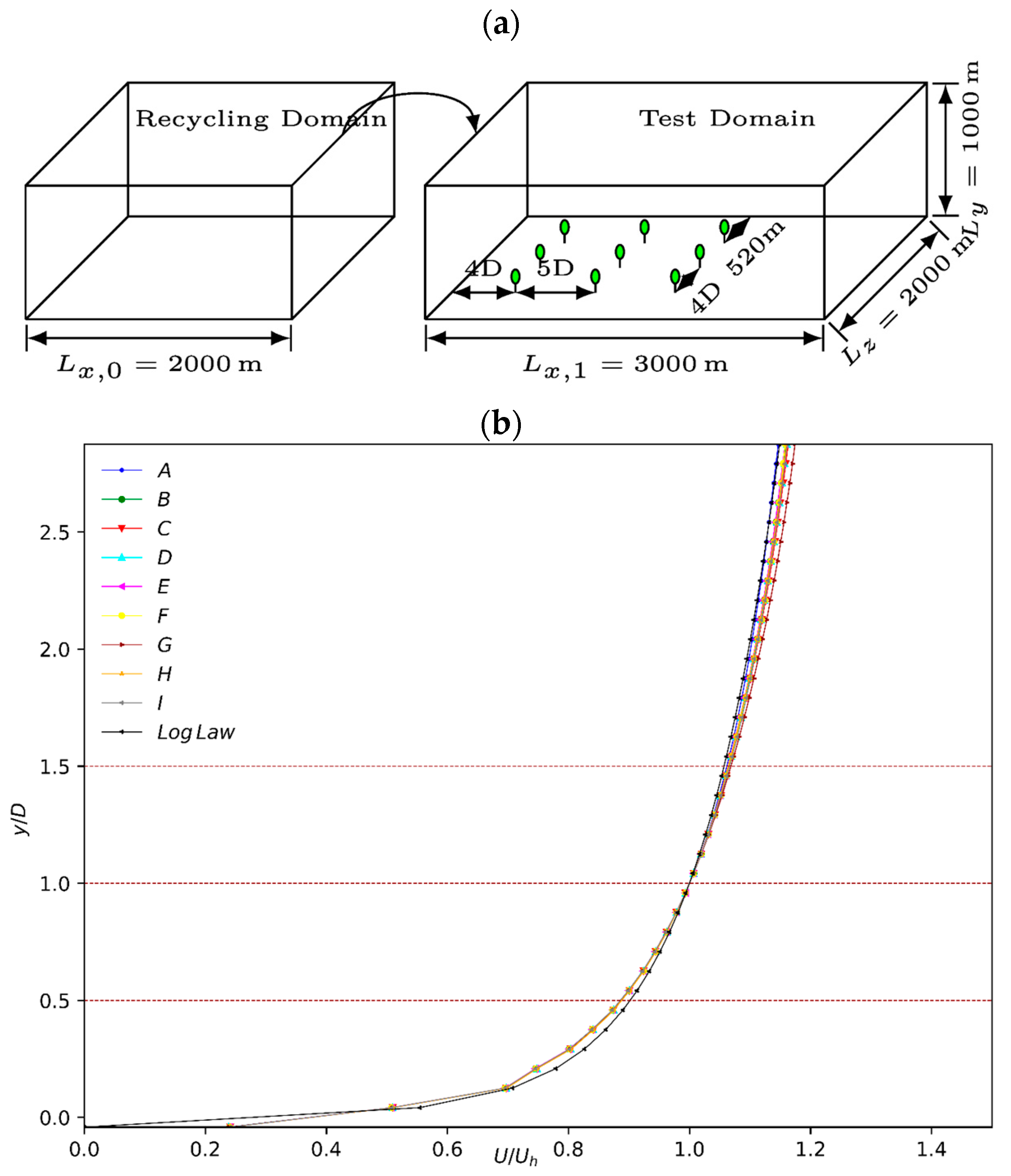
Yaw misalignment was implemented based on [5]. In the presence of yaw, the thrust force was replaced as follows.

$$f=C_T\frac{1}{2}\rho A{\left(U_{\infty }cos\theta \right)}^2$$

(12)

Then the thrust force was projected into the Cartesian coordinates with the x-component and the z-component being the following.

$$f_x=fcos\theta =C_T\frac{1}{2}\rho A{\left(U_{\infty }cos\theta \right)}^{2}cos\theta$$

(13)

$$f_z=fsin\theta =C_T\frac{1}{2}\rho A{\left(U_{\infty }cos\theta \right)}^{2}sin\theta$$

(14)

The thrust force was then incorporated into the respective momentum equation.

2.4. Case Set-Up

A concurrent precursor method (CPM) was implemented in the in-house code, WIND4D [43].

The dimensions for all the cases are depicted in Figure 1a. The grid size in every direction is 10 m. The wind speeds and the yaw angles are listed in

Table 1. All the simulation cases of the present study.

ABL Cases	$\mathbf{Wind}\mathbf{Speeds},{\mathit{U}}_{\mathit{\infty }};\mathit{u}$ (ms−1)	Yaw Angles, γ (°)
case A	7.3; 0.412	30
case B	7.3; 0.412	20
case C	7.3; 0.412	0
case D	10.4; 0.587	30
case E	10.4; 0.587	20
case F	10.4; 0.587	0
case G	4.3; 0.243	30
case H	4.3; 0.243	20
case I	4.3; 0.243	0

. The surface roughness length ($y_0$) of all the cases is 0.1 m, the value typically used for the flat terrains in onshore wind farms. The diameter (D) and hub height ($y_h$) of the turbine are 120 m. The inflow profile from the precursor domain is presented in Figure 1b. All the case profiles are compared against the log law profile; they match well. In the study, each turbine’s thrust coefficient C_T (=3/4) was maintained constant across all cases to primarily investigate the influence of varying wind speeds at different yaw angles.

The flow statistics were collected for over 260 flow-through times. The simulations were run over 70 flow-through times to ensure they reached a fully turbulent state. The time window (T) in the time adaptive wind turbine model was 600 s.

3. Results and Discussion

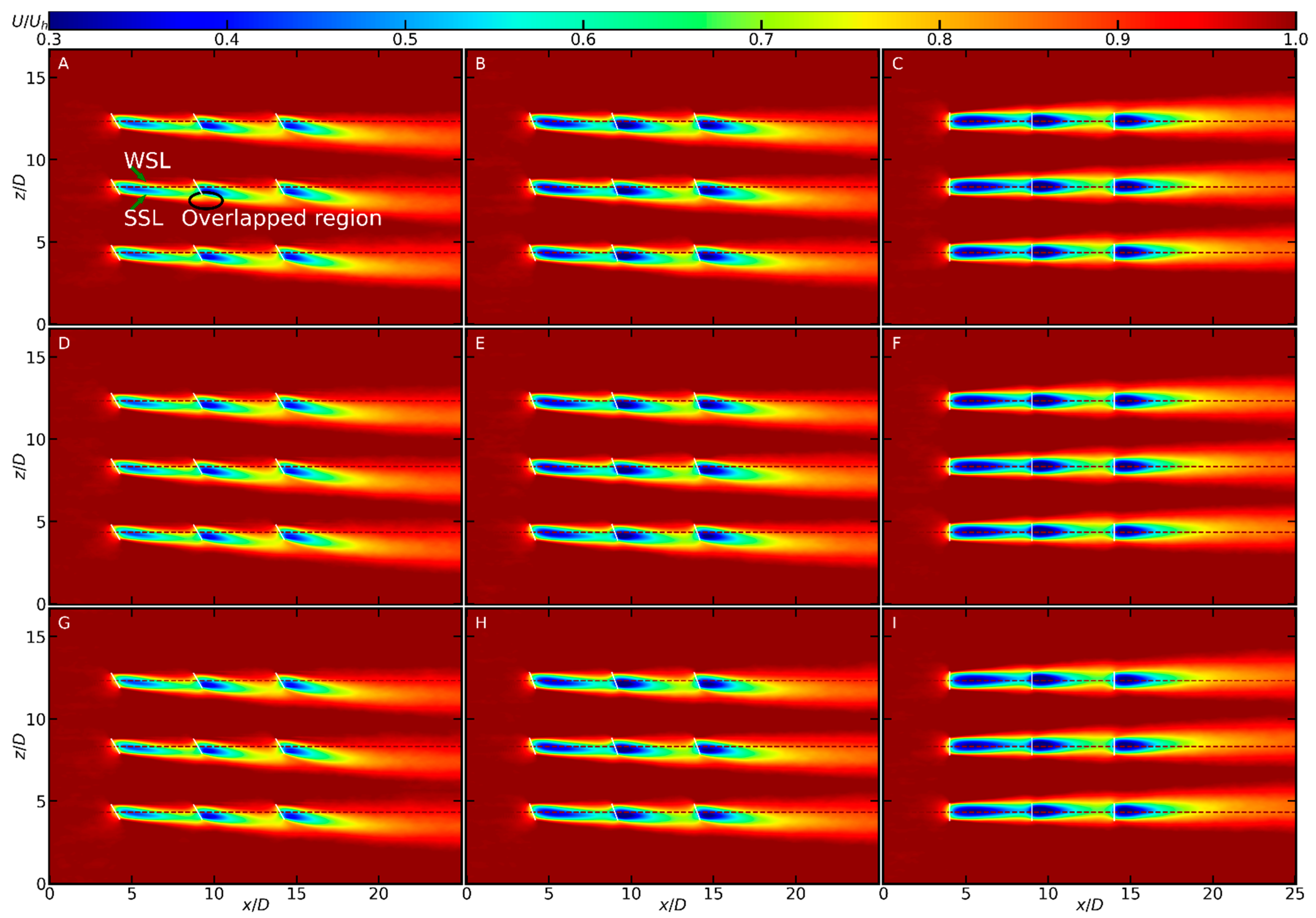
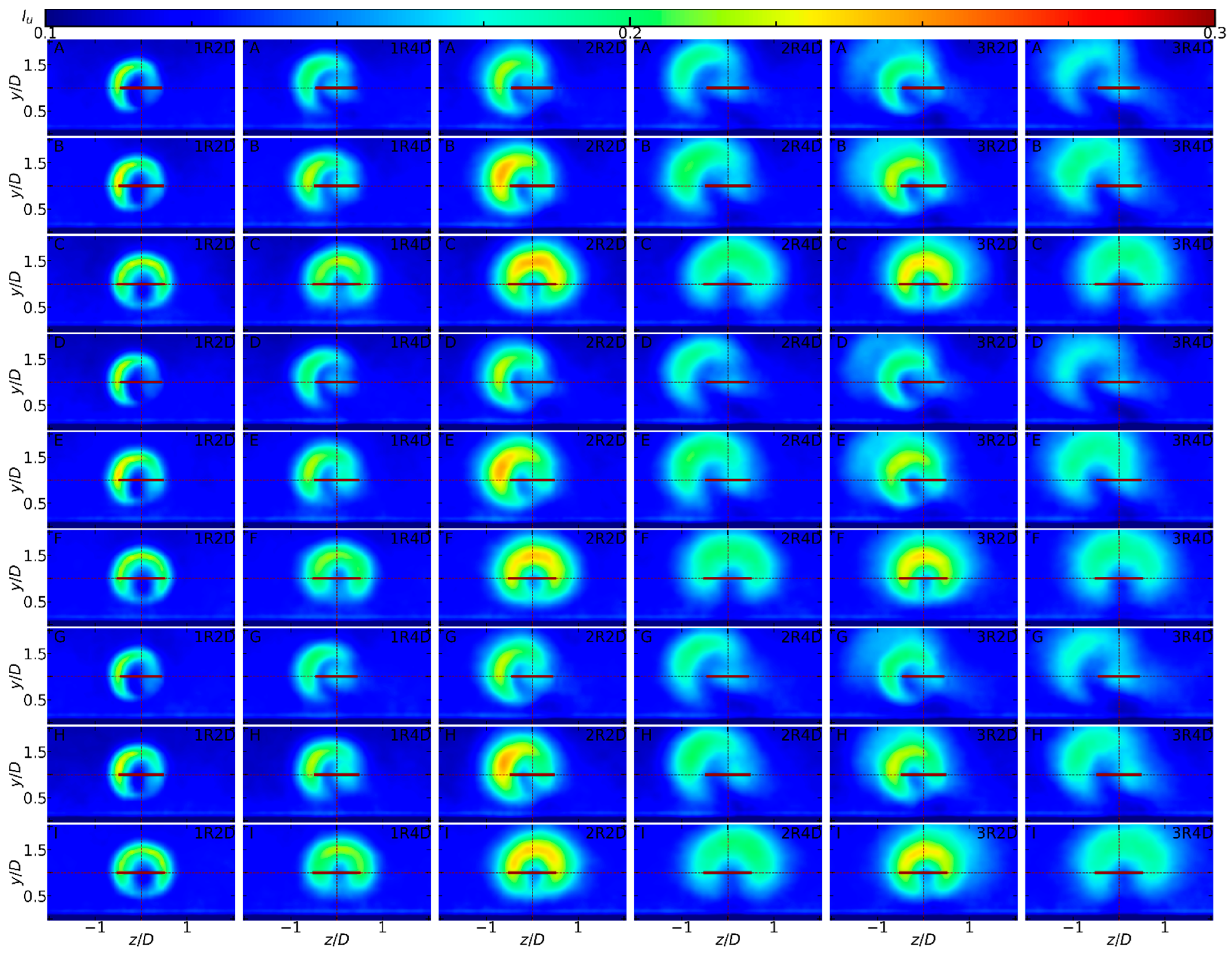
3.1. Analysis of the Contours of the Flow Fields and Turbulence Intensity

Figure 2 displays the time-averaged velocity deficit field in the XZ plane at hub height for all cases, showing how the wake steering affects the deflection of the wake downstream of the wind farm. The secondary effects of the wake steering cause an additional deflection of the wake in the downstream direction of the wind farm. When the turbine converts a portion of the incoming turbulent kinetic energy (TKE) into power output, a low-speed zone (also known as the wake region) forms behind it. The wake then extends downstream and widens due to turbulence mixing, allowing the wind to recover before reaching the next turbine. The momentum exchange between the wake region and the ambient flow increases with increasing yaw angle. However, the relative exchange does not increase significantly with increasing speeds, leading to a little mismatch in self-similarity in velocity deficit profiles (normalized by hub height velocity, U_h).

The velocity deficit contours reveal a high-speed channel of unperturbed velocity containing a significant amount of kinetic energy that passes through space between the columns of the turbine in wind farms for non-yawed cases, as depicted in Figure 2. In contrast, for yawed cases, this energy is extracted more and more as the flow moves downstream with an increasing yaw angle. It is worth noting that even with the largest yaw angles, the lateral wake interactions are minimal to zero. Therefore, the spanwise distance between turbine columns is sufficient to avoid these interactions.

The turbulence intensity distributions in the XZ plane at hub height for all cases are presented in Figure 3. The turbulence intensity is the ratio of the standard deviation, σ_u (or root mean square) of the local fluctuating velocities to the mean unperturbed velocity at hub height, U_h. In all the cases, TI is higher at the wake edges and shear layers due to a higher production rate of turbulent kinetic energy (TKE) than its dissipation. This rise in turbulence levels is primarily due to shear layers and momentum flux transfer from the incoming atmospheric boundary layer into the wake region. The accumulation of TI in the downstream direction leads to a quick recovery of the wakes and a shortening of the near-wake lengths.

A dual-peak turbulence distribution is observed, with enhanced shear layers at the edges of the turbine. Under yawed conditions, this distribution becomes asymmetric, and the asymmetry increases with increasing yaw angles. This results in an asymmetric wake recovery, as evident in the velocity-deficit profiles and contour plots.

Compared to non-yawed cases, yawed cases have more added turbulence (turbine-wake-induced turbulence intensity) downstream. This added turbulence increases wake width with no significant decrease in velocity deficit downstream.

Figure 4 displays the streamwise velocity contours in the YZ plane at 2D and 4D distances from each turbine of each row for all the cases. Yawed cases generate a pair of counter-rotating vortices at the top and bottom of the turbine rotor, and these vortices shift the wakeline away from the center as the wake moves downstream. The vortices eventually turn into a curled shape at further downstream locations. Although the yaw angles significantly influence the shape of the vortices, the influence of wind speeds is insignificant. The curled wake shape becomes more pronounced with increasing yaw angles, and slightly larger vortices are produced at higher wind speeds. That is why the wake moves less from the centerline for lower wind speeds, and this behavior is also evident in Figure 10 further below.

Figure 5 shows the turbulence intensity (TI) of the streamwise velocity in the YZ cross-sectional planes at different downstream positions of the wind farm. The distribution of the TI also exhibits the evolution of the curled shape phenomenon. In the wake of a turbine, the entrainment of surrounding fluid causes a significant impact on the TI of the flow. At the upper edge of the wake, the entrainment of high-momentum fluid from the boundary layer results in an increase in TI due to increased shear and turbulence generation. Conversely, at the lower edge of the wake, the entrainment of low-momentum fluid from the boundary layer leads to a decrease in TI due to reduced shear and turbulence generation.

The displacement of the wake in the XY plane of streamwise velocity is observed to exhibit vertical characteristics, as demonstrated by Figure 6. This displacement is primarily caused by interactions between counter-rotating vortices, the ground, and the rotation of the wake, with the most prominent effects being observed under yawed conditions. The extent of this displacement is directly proportional to the magnitude of the yaw angle. The direction of the displacement depends on the orientation of the counter-rotating vortices, which is a function of the sign of the yaw angle. The vertical displacement of the wake is critical to the overall wake deflection, which is further instrumental in mitigating wake losses downstream. Wind shear differences in the vertical direction exhibit significant variation with changing yaw angles but are relatively small with variations in wind speeds in the wake region. The accelerations at the wake edges are determined to be negligible for all three wind speeds at any specific yaw angles at any downstream position. Given their minimal effects on wake recovery, these accelerations’ contributions to turbines’ power output are also insignificant. The presence of these accelerations under neutral atmospheric conditions is primarily attributed to the adjacent upstream wakes in wind farms.

In a fully developed wake region, the vertical kinetical energy flux brings the high-speed wind down to the upstream of the turbine at the hub height level. This energy flux results from the complex interplay of atmospheric turbulence, wake-induced turbulence, and the cumulative growth of the boundary layer due to wake, as illustrated in Figure 6 and Figure 7. The vertical kinetical energy flux increases as the flow moves downstream, as evident from the increased turbulence levels and boundary layer growth. The turbulence intensity profiles and contour plots consistently indicate elevated turbulence levels near the upper edges of the rotor due to stronger wind shear, which leads to turbulent mixing, eddy formation, and vortex generation.

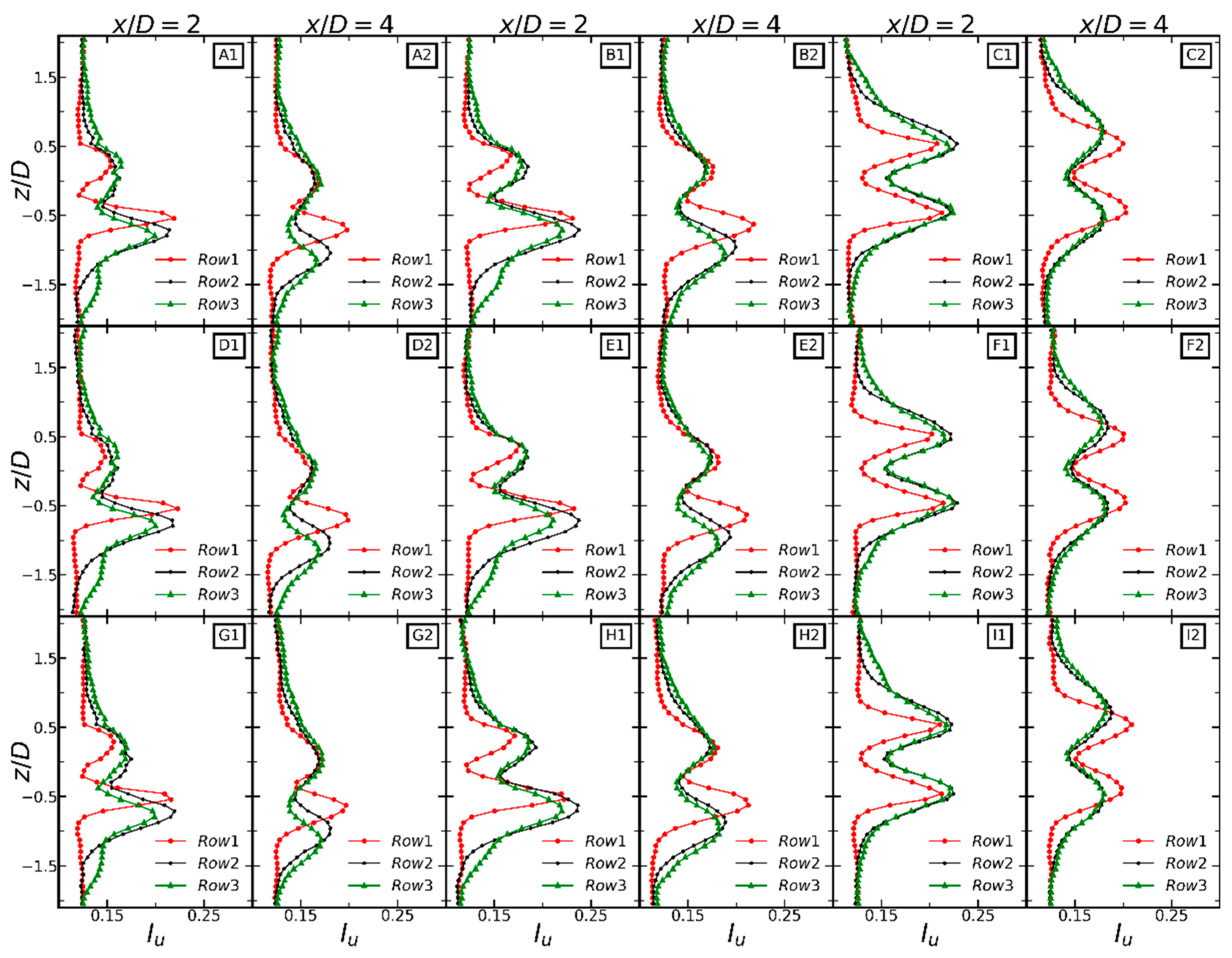
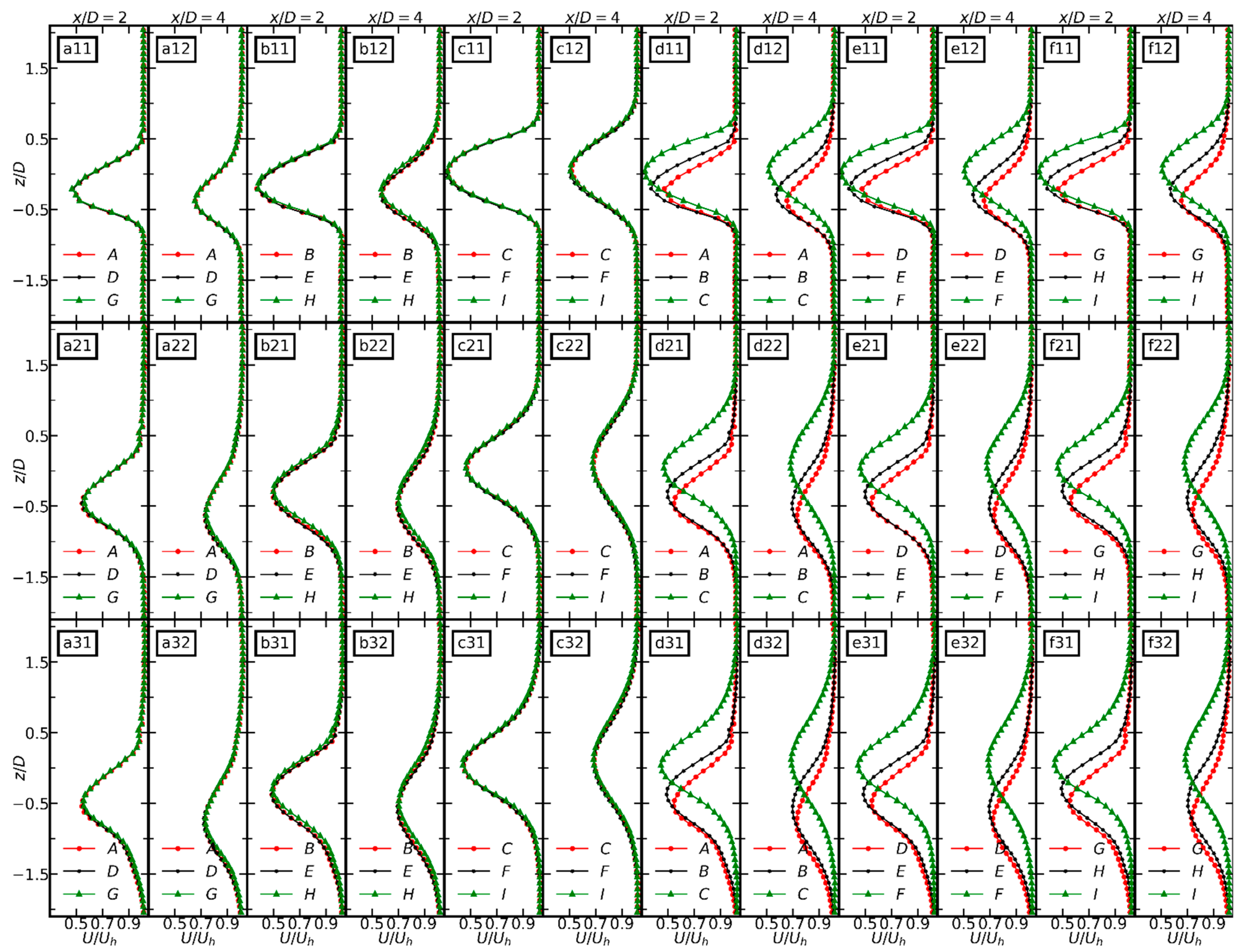
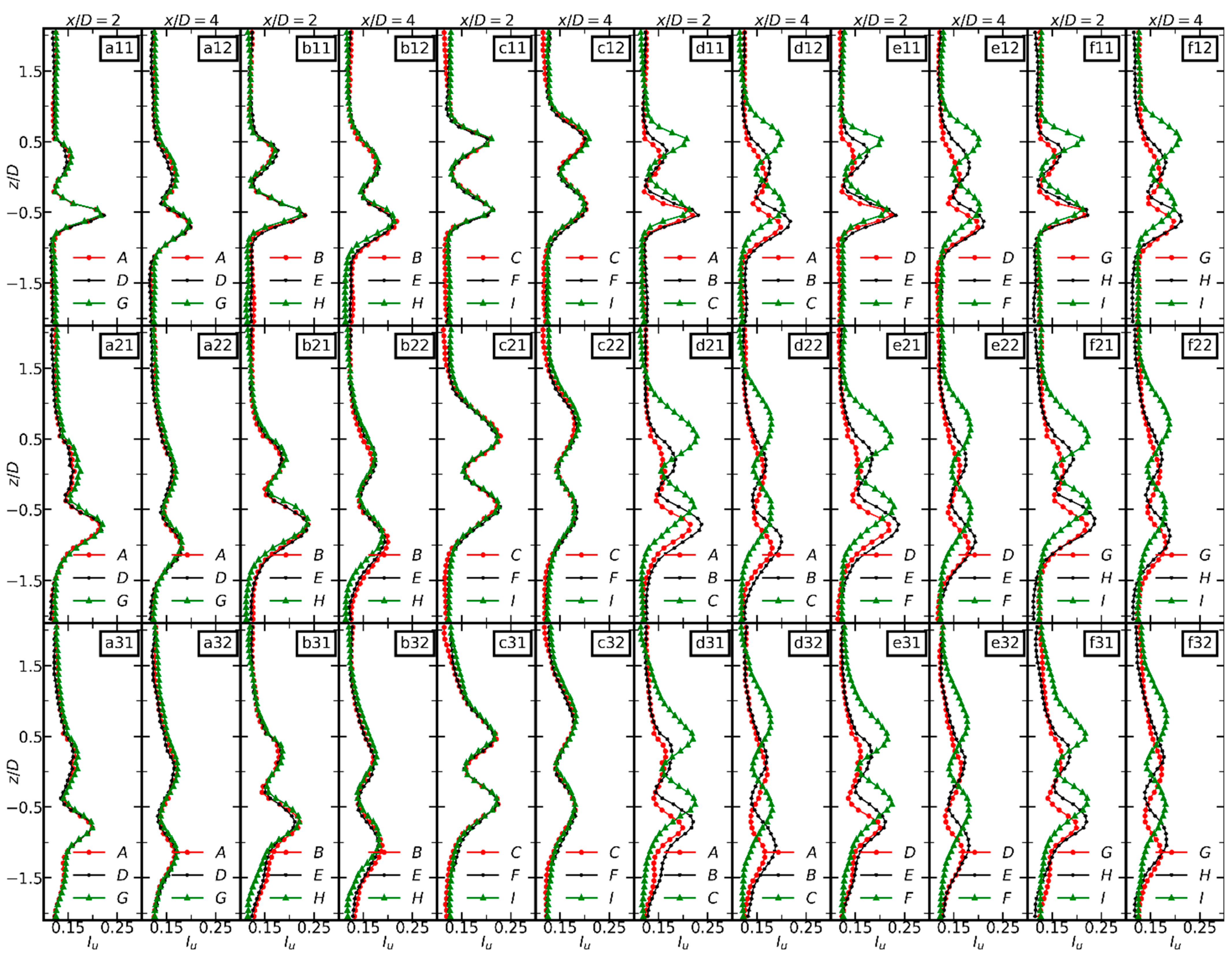
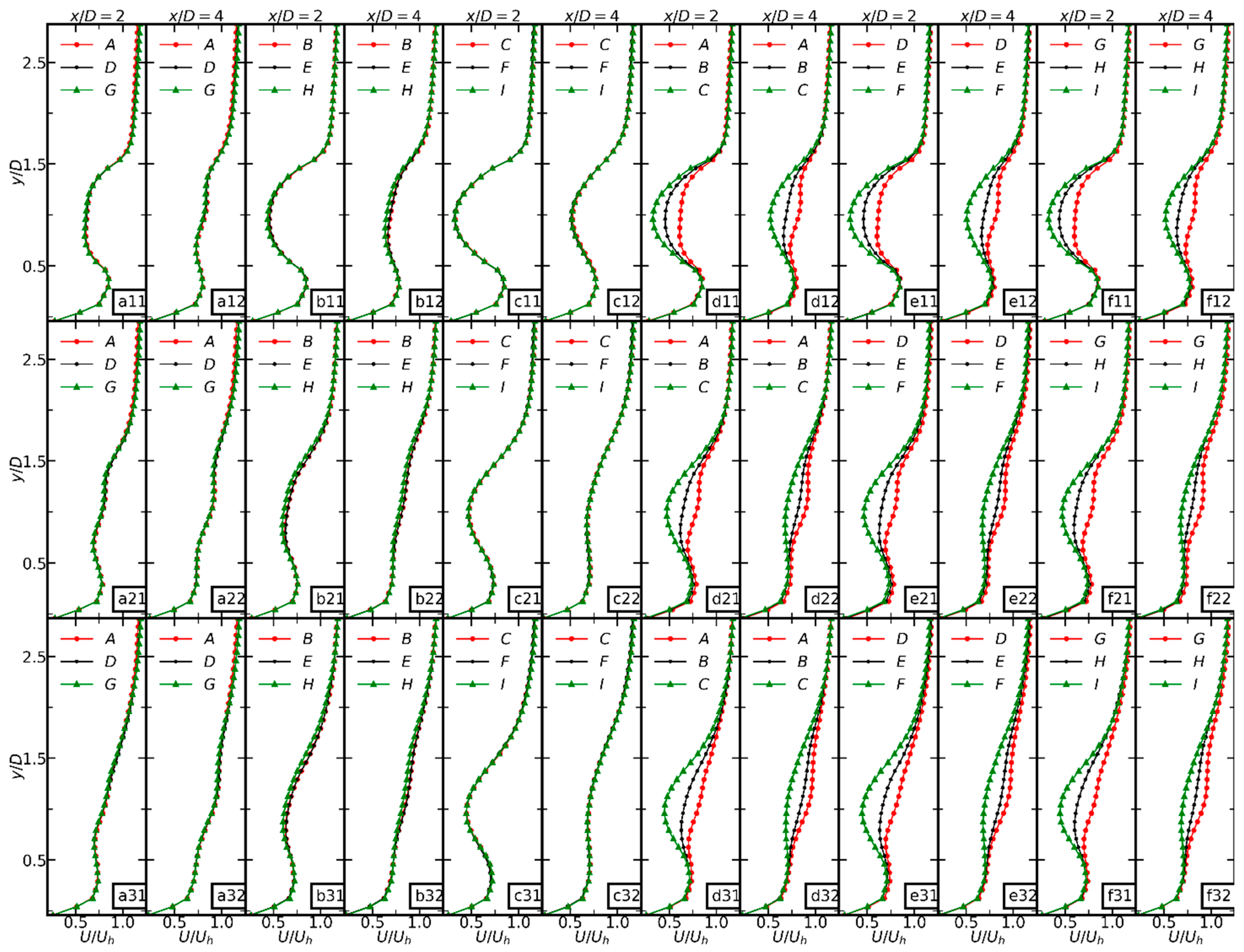
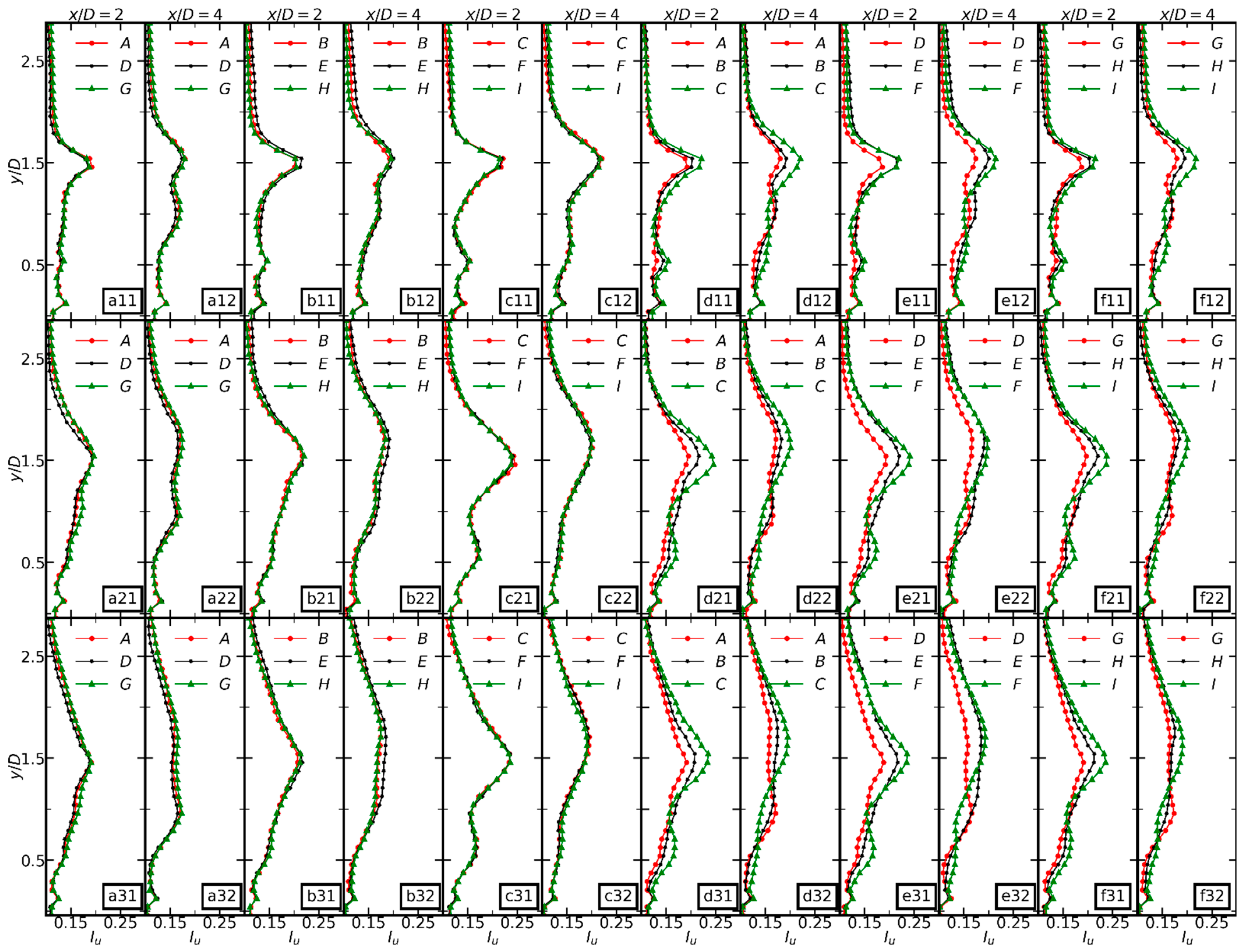
3.2. Analysis of the Plots of the Flow Fields and Turbulence Intensity

Figure 8 presents a comparative assessment of the wake width at downstream locations of 2D and 4D for each row of turbines for all cases studied. The results indicate that the wake width gradually increases beyond 4D downstream of the third row, contributing to the expansion of the wind-farm wake. This phenomenon is attributed to the increased turbulence mixing in the downstream flow by mean-wind advection and turbulent transport. The velocity deficit profiles exhibit a two-dimensional Gaussian axisymmetric behavior for non-yawed cases, consistent with previous research [12,44]. However, the lateral profiles of the yawed cases are non-axisymmetric, and the degree of asymmetry increases as the flow advances downstream and the yaw angle increases. Thus, the wind-farm wake characteristics are influenced by the yaw angle and the downstream distance, and these factors significantly affect the wake width and its expansion.

Figure 9 compares the lateral turbulence intensity profiles for three rows at two downstream positions (2D and 4D) in all cases studied. The results show that, after all three rows, the near-wake region around 2D downstream positions exhibits higher turbulence levels. The TI experiences variations in both magnitude and spatial distribution as the flow progresses downstream. Turbulent mixing reduces the turbine-wake-induced turbulence levels downstream, resulting in a more uniform velocity profile with reduced fluctuations, particularly in the far downstream region where turbulent structures have dissipated and mixed with the mean flow. This diffusion and merging of turbulent fluctuations with the mean flow are responsible for reducing total TI downstream. These findings suggest that the wind-farm wake characteristics are influenced by turbulent mixing and the downstream distance, which affects the spatial distribution and magnitude of TI in the wake region.

The wake losses are observed to be nearly identical for all velocities in the non-yawed cases, as illustrated in Figure 10. This phenomenon is also reflected in the power output results, as depicted in Figure 14 below. Furthermore, Figure 10 highlights that the wake deflection is more prominent for higher speeds in the yawed cases. Given the lesser wake steering for lower speeds, the blockage losses are higher for them. This wake behavior significantly impacts the power output, particularly for the yaw angle of 20°. The relative power output experiences a decline for the lower speeds, particularly for speed 4.3 ms⁻¹. Notably, the difference in the lateral spreads of the wakes for different wind speeds is insignificant even farther downstream of the turbines, especially for higher wind speeds. As the yaw angle reduces, the lateral wake spread becomes more noticeable due to the lesser mixing of momentum of the wake and undisturbed flow from both above and sideways. This characteristic of the wake considerably influences the power output of each turbine.

The turbulence intensity profiles in the XZ plane at hub height exhibit similar trends to the velocity deficits, as illustrated in Figure 10 and Figure 11. The wind speed and yaw angle variations affect the magnitude and location of the maximum TI, influencing wind turbines and wind farms’ performance and efficiency. The elevated wind speeds displace the maximum TI away from its original position due to increased mixing and turbulence, leading to downstream expansion and shift of the wake. The profiles exhibit more deflection as the wind speeds increase, particularly for the yaw angle of 20°. As the flow convects further downstream, the difference in the deflection of the profiles becomes more noticeable with the change in wind speeds at any yaw angle. This wake behavior can more significantly impact power output when additional turbine rows are placed after the third row, and the difference in power output can be more pronounced.

The impact of wind speed on the vertical velocity deficits is shown in Figure 12, which indicates that there is only a weak correlation between these two parameters, except for the yaw angle of 20°. Typically, weaker shear layers are formed at lower wind speeds, resulting in less mixing between the wake region and the incoming atmospheric boundary layer. This wake behavior significantly impacts power output, as illustrated in Figure 14. However, the effects of this behavior are mitigated in the far wake region by the lateral transport of the flow.

The results presented in Figure 13 indicate that the vertical turbulence intensity profiles do not exhibit a significant dependence on wind speed variations for different yaw angles. However, changes in yaw angles affect the TI profiles at any specific wind speed. Increasing yaw angles increases turbulence levels, particularly at the turbine edges. Mixing wake turbulence with lateral turbulence in the far wake region mitigates these effects, leading to wake recovery. On the other hand, stronger shear introduces more momentum into the wake, resulting in more eddies and vortices, thereby increasing turbulence intensities when the shear is stronger.

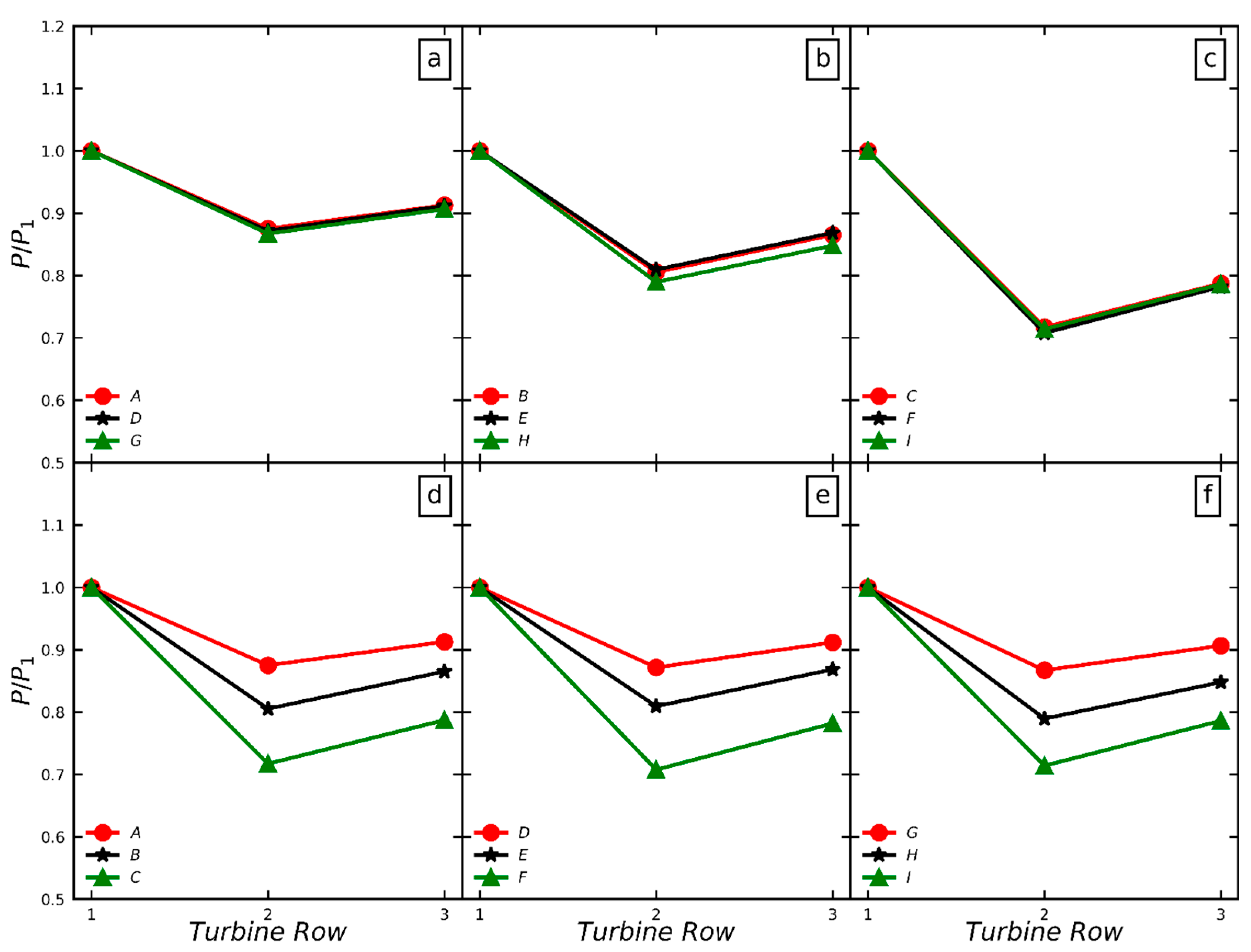
3.3. Analysis of the Relative Power Output of Wind Farms

In Figure 14, the power output of turbines within the wind farm is presented, which has been normalized by the power output of a representative upstream turbine. The power values have been averaged over time and across the same row of turbines. The analysis investigates the effect of different yaw angles at various wind speeds on the power output of the turbines.

The variability in incoming turbulence has been identified as a potential factor contributing to the observed difference in power output between the second and third rows of wind turbines. This can be attributed to the fact that turbulence can significantly impact the efficiency of wind turbines by causing unpredictable wind speeds, which can lead to reduced power output. In all cases considered, the power output of the second row of turbines was found to be lower than that of the third row. This trend can be explained by the relatively slow recovery of wakes behind the first row, which is characterized by a high-velocity deficit and low turbulence levels, compared to the second row. Beyond the second row, however, the increased turbulence levels facilitate a faster recovery of wakes, resulting in greater power generation. These findings highlight the importance of considering turbulence levels and wake dynamics in optimizing the design and placement of wind turbines for maximum power generation.

In the absence of yaw misalignment of turbines, full wake interactions demonstrate weak dependence on wind speeds. Similarly, partial wake interactions exhibit limited sensitivity to wind speeds for a yaw angle of 30°. However, when the turbines are yawed at 20°, partial wake interactions show a slightly stronger dependence on wind speeds, particularly at lower wind speeds. Notably, at wind speeds of 4.3 ms⁻¹, the relative partial wake interactions are comparatively stronger for lower wind speeds. The downstream turbines’ gradual decrease in power output indicates that greater momentum extraction from the fluid flow than entrainment occurs. These wake interactions’ impact is evident in the power output of wind turbines, as depicted in Figure 14.

4. Conclusions

In this study, we performed nine large eddy simulation (LES) cases of the neutrally stratified atmospheric boundary layer (ABL) flow through a three-by-three wind farm. The study’s primary purpose was to analyze the effects of the variability of wind speeds at different yaw angles on the wind farm’s wake characteristics and power output. All the LESs cases have almost the same turbulence intensity of 12.0% at hub height, and the three wind speeds are about 7.3 ms⁻¹, 10.4 ms⁻¹, 4.3 ms⁻¹, and the three yaw angles are 30°, 20°, and 0°. Wind speed variations have little influence in wake characteristics for any yaw angle, except for the wind speed 4.3 ms⁻¹ at the yaw angle of 20°. The wake deflection is higher at higher wind speeds and with yawed wind turbines. However, the degree of wake steering is reduced at lower wind speeds, resulting in increased blockage losses. At lower wind speeds, the turbulence intensity profiles show reduced deflection, particularly at the yaw angle of 20 degrees when the wind speed is 4.3 ms⁻¹. As the flow progresses downstream, the difference in the degree of deflection between the profiles becomes more apparent, regardless of the yaw angle, due to the varying wind speeds. This wake behavior significantly affects the power generated, especially when the turbines are yawed. The power losses are higher for the lower wind speeds, especially for the yaw angle of 20° at the wind speed of 4.3 ms⁻¹.

References

1. Allen, M.; Babiker, M.; Chen, Y.; de Coninck, H.; Connors, S.; van Diemen, R.; Dube, O.; Ebi, K.; Engelbrecht, F.; IPCC; et al. Summary for Policymakers. In Global Warming of 1.5 °C; An IPCC Special Report; IPCC: Geneva, Switzerland, 2018. [Google Scholar]
2. Medici, D.; Dahlberg, J.Å. Potential Improvement of Wind Turbine Array Efficiency by Active Wake Control (AWC). In Proceedings of the European Wind Energy Conference and Exhibition, Madrid, Spain, 16–19 June 2003; Department of Mechanics, The Royal Institute of Technology: Gottingen, Germany, 2003; pp. 65–84. [Google Scholar]
3. Adaramola, M.S.; Krogstad, P.-Å. Experimental Investigation of Wake Effects on Wind Turbine Performance. Renew. Energy 2011, 36, 2078–2086. [Google Scholar] [CrossRef]
4. Gebraad, P.M.O.; Teeuwisse, F.W.; van Wingerden, J.W.; Fleming, P.A.; Ruben, S.D.; Marden, J.R.; Pao, L.Y. Wind Plant Power Optimization through Yaw Control Using a Parametric Model for Wake Effects—A CFD Simulation Study. Wind Energy 2016, 19, 95–114. [Google Scholar] [CrossRef]
5. Jiménez, Á.; Crespo, A.; Migoya, E. Application of a LES Technique to Characterize the Wake Deflection of a Wind Turbine in Yaw. Wind Energy 2010, 13, 559–572. [Google Scholar] [CrossRef]
6. Wu, Y.-T.; Lin, C.-Y.; Chang, T.-J. Effects of Inflow Turbulence Intensity and Turbine Arrangements on the Power Generation Efficiency of Large Wind Farms. Wind Energy 2020, 23, 1640–1655. [Google Scholar] [CrossRef]
7. Churchfield, M.J.; Lee, S.; Michalakes, J.; Moriarty, P.J. A Numerical Study of the Effects of Atmospheric and Wake Turbulence on Wind Turbine Dynamics. J. Turbul. 2012, 13, N14. [Google Scholar] [CrossRef]
8. Larsen, G.C.; Madsen, H.A.; Thomsen, K.; Larsen, T.J. Wake Meandering: A Pragmatic Approach. Wind Energy 2008, 11, 377–395. [Google Scholar] [CrossRef]
9. Mishnaevsky, L.; Hasager, C.B.; Bak, C.; Tilg, A.-M.; Bech, J.I.; Doagou Rad, S.; Fæster, S. Leading Edge Erosion of Wind Turbine Blades: Understanding, Prevention and Protection. Renew. Energy 2021, 169, 953–969. [Google Scholar] [CrossRef]
10. Carraro, M.; De Vanna, F.; Zweiri, F.; Benini, E.; Heidari, A.; Hadavinia, H. CFD Modeling of Wind Turbine Blades with Eroded Leading Edge. Fluids 2022, 7, 302. [Google Scholar] [CrossRef]
11. Medici, D.; Alfredsson, P.H. Measurements on a Wind Turbine Wake: 3D Effects and Bluff Body Vortex Shedding. Wind Energy 2006, 9, 219–236. [Google Scholar] [CrossRef]
12. Chamorro, L.P.; Porté-Agel, F. A Wind-Tunnel Investigation of Wind-Turbine Wakes: Boundary-Layer Turbulence Effects. Bound. Layer Meteorol. 2009, 132, 129–149. [Google Scholar] [CrossRef] [Green Version]
13. Wu, Y.-T.; Porté-Agel, F. Large-Eddy Simulation of Wind-Turbine Wakes: Evaluation of Turbine Parametrisations. Bound. Layer Meteorol. 2011, 138, 345–366. [Google Scholar] [CrossRef]
14. Howland, M.F.; Bossuyt, J.; Martínez-Tossas, L.A.; Meyers, J.; Meneveau, C. Wake Structure in Actuator Disk Models of Wind Turbines in Yaw under Uniform Inflow Conditions. J. Renew. Sustain. Energy 2016, 8, 043301. [Google Scholar] [CrossRef] [Green Version]
15. Fleming, P.A.; Gebraad, P.M.O.; Lee, S.; van Wingerden, J.-W.; Johnson, K.; Churchfield, M.; Michalakes, J.; Spalart, P.; Moriarty, P. Evaluating Techniques for Redirecting Turbine Wakes Using SOWFA. Renew. Energy 2014, 70, 211–218. [Google Scholar] [CrossRef]
16. Bastankhah, M.; Porté-Agel, F. Experimental and Theoretical Study of Wind Turbine Wakes in Yawed Conditions. J. Fluid Mech. 2016, 806, 506–541. [Google Scholar] [CrossRef]
17. Shapiro, C.R.; Gayme, D.F.; Meneveau, C. Modelling Yawed Wind Turbine Wakes: A Lifting Line Approach. J. Fluid Mech. 2018, 841, R1. [Google Scholar] [CrossRef] [Green Version]
18. Qian, G.-W.; Ishihara, T. A New Analytical Wake Model for Yawed Wind Turbines. Energies 2018, 11, 665. [Google Scholar] [CrossRef] [Green Version]
19. Aitken, M.L.; Lundquist, J.K. Utility-Scale Wind Turbine Wake Characterization Using Nacelle-Based Long-Range Scanning Lidar. J. Atmos. Ocean. Technol. 2014, 31, 1529–1539. [Google Scholar] [CrossRef]
20. Maeda, T.; Kamada, Y.; Murata, J.; Yonekura, S.; Ito, T.; Okawa, A.; Kogaki, T. Wind Tunnel Study on Wind and Turbulence Intensity Profiles in Wind Turbine Wake. J. Therm. Sci. 2011, 20, 127–132. [Google Scholar] [CrossRef]
21. Troldborg, N.; Sørensen, J.N.; Mikkelsen, R. Actuator Line Simulation of Wake of Wind Turbine Operating in Turbulent Inflow. J. Phys: Conf. Ser. 2007, 75, 012063. [Google Scholar] [CrossRef]
22. Wu, Y.-T.; Porté-Agel, F. Atmospheric Turbulence Effects on Wind-Turbine Wakes: An LES Study. Energies 2012, 5, 5340–5362. [Google Scholar] [CrossRef] [Green Version]
23. Chamorro, L.P.; Porté-Agel, F. Effects of Thermal Stability and Incoming Boundary-Layer Flow Characteristics on Wind-Turbine Wakes: A Wind-Tunnel Study. Bound.Layer Meteorol. 2010, 136, 515–533. [Google Scholar] [CrossRef] [Green Version]
24. Zhang, W.; Markfort, C.D.; Porté-Agel, F. Near-Wake Flow Structure Downwind of a Wind Turbine in a Turbulent Boundary Layer. Exp. Fluids 2012, 52, 1219–1235. [Google Scholar] [CrossRef] [Green Version]
25. Iungo, G.V.; Wu, Y.-T.; Porté-Agel, F. Field Measurements of Wind Turbine Wakes with Lidars. J. Atmos. Ocean. Technol. 2013, 30, 274–287. [Google Scholar] [CrossRef] [Green Version]
26. Porté-Agel, F.; Wu, Y.-T.; Lu, H.; Conzemius, R.J. Large-Eddy Simulation of Atmospheric Boundary Layer Flow through Wind Turbines and Wind Farms. J. Wind. Eng. Ind. Aerodyn. 2011, 99, 154–168. [Google Scholar] [CrossRef]
27. Li, Q.; Murata, J.; Endo, M.; Maeda, T.; Kamada, Y. Experimental and Numerical Investigation of the Effect of Turbulent Inflow on a Horizontal Axis Wind Turbine (Part II: Wake Characteristics). Energy 2016, 113, 1304–1315. [Google Scholar] [CrossRef]
28. Wiser, R.H.; Bolinger, M. 2018 Wind Technologies Market Report; LBL Publications: Bingley, UK, 2019. [Google Scholar]
29. Stathopoulos, T.; Alrawashdeh, H.; Al-Quraan, A.; Blocken, B.; Dilimulati, A.; Paraschivoiu, M.; Pilay, P. Urban Wind Energy: Some Views on Potential and Challenges. J. Wind. Eng. Ind. Aerodyn. 2018, 179, 146–157. [Google Scholar] [CrossRef]
30. Al-Quraan, A.; Stathopoulos, T.; Pillay, P. Comparison of Wind Tunnel and on Site Measurements for Urban Wind Energy Estimation of Potential Yield. J. Wind. Eng. Ind. Aerodyn. 2016, 158, 1–10. [Google Scholar] [CrossRef] [Green Version]
31. Bataineh, K.M.; Dalalah, D. Assessment of Wind Energy Potential for Selected Areas in Jordan. Renew. Energy 2013, 59, 75–81. [Google Scholar] [CrossRef]
32. Al-Quraan, A.; Al-Mhairat, B. Intelligent Optimized Wind Turbine Cost Analysis for Different Wind Sites in Jordan. Sustainability 2022, 14, 3075. [Google Scholar] [CrossRef]
33. Li, Q.; Jia, H.; Qiu, Q.; Lu, Y.; Zhang, J.; Mao, J.; Fan, W.; Huang, M. Typhoon-Induced Fragility Analysis of Transmission Tower in Ningbo Area Considering the Effect of Long-Term Corrosion. Appl. Sci. 2022, 12, 4774. [Google Scholar] [CrossRef]
34. Fleming, P.A.; Ning, A.; Gebraad, P.M.O.; Dykes, K. Wind Plant System Engineering through Optimization of Layout and Yaw Control. Wind Energy 2016, 19, 329–344. [Google Scholar] [CrossRef] [Green Version]
35. Machielse, L.; Schepers, J.; Wagenaar, J. Controlling Wind in ECN‘s Scaled Wind Farm; EWEA: Copenhagen, Denmark, 2012. [Google Scholar]
36. Fleming, P.; Annoni, J.; Shah, J.J.; Wang, L.; Ananthan, S.; Zhang, Z.; Hutchings, K.; Wang, P.; Chen, W.; Chen, L. Field Test of Wake Steering at an Offshore Wind Farm. Wind Energy Sci. 2017, 2, 229–239. [Google Scholar] [CrossRef] [Green Version]
37. Howland, M.F.; Lele, S.K.; Dabiri, J.O. Wind Farm Power Optimization through Wake Steering. Proc. Natl. Acad. Sci. USA 2019, 116, 14495–14500. [Google Scholar] [CrossRef] [PubMed] [Green Version]
38. Simley, E.; Fleming, P.; Girard, N.; Alloin, L.; Godefroy, E.; Duc, T. Results from a Wake-Steering Experiment at a Commercial Wind Plant: Investigating the Wind Speed Dependence of Wake-Steering Performance. Wind Energy Sci. 2021, 6, 1427–1453. [Google Scholar] [CrossRef]
39. Bou-Zeid, E.; Meneveau, C.; Parlange, M. A Scale-Dependent Lagrangian Dynamic Model for Large Eddy Simulation of Complex Turbulent Flows. Phys. Fluids 2005, 17, 025105. [Google Scholar] [CrossRef] [Green Version]
40. Deardorff, J.W. A Numerical Study of Three-Dimensional Turbulent Channel Flow at Large Reynolds Numbers. J. Fluid Mech. 1970, 41, 453–480. [Google Scholar] [CrossRef]
41. Falgout, R.D.; Yang, U.M. Hypre: A Library of High Performance Preconditioners. In Proceedings of the Computational Science—ICCS, Amsterdam, The Netherlands, 21–24 April 2002; Sloot, P.M.A., Hoekstra, A.G., Tan, C.J.K., Dongarra, J.J., Eds.; Springer: Berlin/Heidelberg Germany, 2002; pp. 632–641. [Google Scholar]
42. Sørensen, J.N.; Myken, A. Unsteady Actuator Disc Model for Horizontal Axis Wind Turbines. J. Wind. Eng. Ind. Aerodyn. 1992, 39, 139–149. [Google Scholar] [CrossRef]
43. Das, R.; Lee, S. Numerical Perspectives on Wind Turbine Wakes. In Proceedings of the 72nd Annual Meeting of the APS Division of Fluid Dynamics, Seattle, WT, USA, 23–26 November 2019. [Google Scholar]
44. Bastankhah, M.; Porté-Agel, F. A New Analytical Model for Wind-Turbine Wakes. Renew. Energy 2014, 70, 116–123. [Google Scholar] [CrossRef]
Figure 1. Sketch of the computation domain consisting of a recycling domain and a test domain (a). Inflow profile from the precursor domain (b).
Energies 16 04953 g001
Figure 2. Visualization of wake of all the cases at hub height in XZ plane. The diameter normalizes all the dimensions. The white and maroon lines represent the turbines and the connected centers of the turbines in a column, respectively.
Energies 16 04953 g002
Figure 3. Turbulence intensity contours of the XZ planes at hub height of all the cases.
Energies 16 04953 g003
Figure 4. Contour of the streamwise velocity deficits of the YZ plane at two downstream positions of each row for all the cases. In the labels “xRyD”, x and y represent the row number and the downstream distance from the same row, respectively.
Energies 16 04953 g004
Figure 5. Contour of the turbulence intensity of the YZ plane at two downstream positions of each row for all the cases.
Energies 16 04953 g005
Figure 6. Contour of the velocity deficits of the XY plane for all the cases.
Energies 16 04953 g006
Figure 7. Contour of the turbulence intensity of the XY plane for all the cases.
Energies 16 04953 g007
Figure 8. Comparison of velocity deficits among the rows at two downstream positions for all the cases. (A1,A2) refer to two downstream positions (2D, 4D) of case A, others (B1,B2,C1,C2,D1,D2,E1,E2,F1,F2,G1,G2,H1,H2,I1,I2) follow the same pattern.
Energies 16 04953 g008
Figure 9. Comparison of turbulence intensity; the rows at two downstream positions for all the cases.
Energies 16 04953 g009
Figure 10. Comparison of the velocity deficits for different yaw angles and wind speeds, at downstream, for the three rows. Each row in the figure refers to each row of the wind farm.
Energies 16 04953 g010
Figure 11. Comparison of the turbulence intensity for different yaw angles and wind speeds, at downstream, for the three rows. Each row in the figure refers to each row of the wind farm.
Energies 16 04953 g011
Figure 12. Comparison of the vertical profiles of velocity deficits for different yaw angles and wind speeds, at downstream, for the three rows. Each row in the figure refers to each row of the wind farm.
Energies 16 04953 g012
Figure 13. Comparison of the vertical profiles of turbulence intensity for different yaw angles and wind speeds, at downstream, for the three rows. Each row in the figure refers to each row of the wind farm.
Energies 16 04953 g013
Figure 14. Relative power output comparisons for the different speeds and yaw-angles. The subfigures (ac) refer to the comparison among three wind speeds at 30°, 20°, and 0° yaw angles, respectively. The subfigures (df) compare three yaw angles at 7.3 ms−1, 10.4 ms−1, and 4.3 ms−1 wind speeds, respectively.
Energies 16 04953 g014