Economic Load-Reduction Strategy of Central Air Conditioning Based on Convolutional Neural Network and Pre-Cooling

Abstract

Central air conditioning in large buildings is an important demand-response resource due to its large load power and strong controllability. Demand-response-oriented air conditioning load modeling needs to calculate the room temperature. The room temperature calculation models commonly used in the existing research cannot easily and accurately calculate the room temperature change of large buildings. Therefore, in order to obtain the temperature change of a large building and its corresponding power potential, this paper first proposes a building model based on CNN (convolutional neural network). Then, in order to fully apply the demand-response potential of the central air conditioning load, this paper puts forward an evaluation method of the load-reduction potential of the central air conditioning cluster based on pre-cooling and develops an economic load-reduction strategy according to the different energy consumption of different buildings in the pre-cooling stage. Finally, multiple building examples with different building parameters and temperature comfort ranges are set up, and the economic advantages of the proposed strategy are illustrated by Cplex solution examples.

1. Introduction

With the increasing population in large cities, the peak of the urban electricity load is increasing. Among this load, air conditioning, as a major consumer of electricity in summer, accounts for 30% to 40% of the peak load [1]. Buildings have a certain heat-storage capacity, so in order to alleviate the peak pressure of the power system, the air conditioning load can be shifted in a short time by means of pre-cooling, temporary shutdown, etc., to achieve the purpose of load reduction within the specified time period and without affecting the comfort of users.

This section firstly reviews the existing research from three aspects: the building model [2,3,4,5,6,7,8,9], the central air conditioning energy consumption model [10,11,12,13,14,15,16], and the application of central air conditioning in power system demand response [17,18,19,20,21,22,23,24,25]. Then, it summarizes the challenges of central air conditioning participating in power system demand response and points out the contributions made by this research.

The central air conditioning model for demand response mainly includes the room temperature calculation model and energy consumption calculation model. The commonly used models for calculating room temperature include the equivalent thermal parameter (ETP) model and resistance–capacitance (RC) network model. Reference [2] discretized the second-order ETP model and identified the parameters of the second-order ETP model by genetic algorithm (GA). Reference [3] proposes a data-driven online parameter-identification method for a variable-frequency air conditioning load model and used particle swarm 0ptimization (PSO) to solve it. Based on the first-order model, reference [4] conducted regression analysis on historical indoor and outdoor temperature and air conditioning energy consumption data and identified model parameters. References [5,6,7] derived the energy storage model of fixed-frequency air conditioners based on the ETP model and obtained the recurrence equation of the air conditioner energy storage model SOC according to the characteristic of the constant energy efficiency ratio of fixed-frequency air conditioners. The ETP model has the advantages of fewer parameters, less computation, and easy programming. However, because it cannot take into account the temperature difference and heat exchange of different cooling areas in the building, it is not suitable for large buildings. References [8,9] used the RC network model to model the whole building from a single room and applied the model to the optimal scheduling of intelligent buildings. The RC network model can consider the building topology, but the program is difficult to implement and requires many measuring points to identify the model parameters. Therefore, in view of the above technical drawbacks, this paper proposes a convolutional neural network (CNN)-based building model, which can consider the temperature differences and heat exchange in different cooling zones, and the number of measurement points required for modeling is reduced compared with the RC network model.

According to the different types of air conditioners, the energy consumption model of air conditioners also has different forms. The compressor power and cooling capacity of fixed-frequency air conditioners are not adjustable, and a constant energy efficiency ratio (electric heating conversion coefficient) is usually used to describe the relationship between energy consumption and cooling capacity [10,11]. Variable-frequency air conditioners can adjust energy consumption and cooling capacity by adjusting the frequency of the compressor and usually adopt polynomials to fit the relationship between the cooling capacity, power, and frequency of the compressor [12,13]. Central air conditioning systems usually include chilled water pumps, cooling water pumps, fan coils, cooling towers, and chiller units. Reference [14] used a BP neural network to establish a load forecasting model of central air conditioning. For a certain cooling load, there are many possible operating conditions of the central air conditioning system for meeting the cooling demand, and the energy consumption of these conditions is different, so there is the problem of working condition optimization. References [15,16] used a polynomial to fit the experimental data, obtained the energy consumption model of the central air conditioning system, and established the energy-saving operation strategy of the central air conditioning system. It can be seen that the energy consumption model of central air conditioning has nonlinear characteristics, and applying it directly to the optimization of scheduling will bring difficulties in finding the solution to the problem. Therefore, the paper obtains a linearized energy consumption model of central air conditioning by solving the optimal condition in advance and segmentally linearizing the “cooling capacity minimum energy consumption” curve under the optimal condition.

Through the formulation of reasonable scheduling strategies, air conditioning loads can provide auxiliary services for the power system, such as frequency regulation, peak shaving, power fluctuation reduction of the tie line, fluctuation reduction of renewable energy, and maximum consumption of renewable energy [17,18,19,20,21,22,23,24,25]. Based on the second-order ETP model, reference [19] established a load-reduction strategy with alternative start-stop of the central air conditioning clusters. However, the second-order ETP model only describes the equivalent temperature of the whole building and cannot describe the temperature of each room separately. Even though the ETP-equivalent temperature in the scheduling process can meet the comfort requirements (within the allowed temperature range), it does not mean that the temperatures of all individual rooms meet the comfort requirements, and there may still be individual room temperatures beyond the allowed temperature range. Reference [25] evaluated the load-reduction potential of central air conditioning, analyzed the impact factors in detail, and proposed an operation mode under the specified load-reduction capacity. However, when the target load-reduction value of the central air conditioning cluster is lower than the maximum load-reduction potential, the operation mode of the central air conditioning cluster is not unique, and the proposed model could not guarantee the optimal operation.

It can be seen that when central air conditioning is applied to demand-response scheduling (this paper refers to load reduction within a specified period), it will face the following challenges: (1) The first regards how to establish a relatively simple and more accurate building temperature model. For the ETP model, its building temperature calculation is inaccurate due to not taking into account the temperature difference and heat exchange in different areas. The RC network model indeed considers the temperature difference and heat exchange in different areas; however, with the increase of building scale, the complexity of the RC network model increases rapidly due to numerous increased room parameters. Therefore, it is difficult to establish the RC network model for large-scale buildings. The advantages and disadvantages of the RC network model and the ETP model are summarized in

Table 1. Summary of the advantages and disadvantages of building temperature models.

Model	Calculation Time	Parameter Number	Calculation Accuracy
Second-order ETP model	Short	4, Irrelated to the scale of the building.	Inaccurate: The temperature of each room may exceed the comfort range.
RC network model	Long	Uncertainty, Related to the building scale; increases significantly with the scale.	Accurate: The comfort of each room is ensured.

. In this paper, a building temperature model is established based on CNN with the consideration of room heat exchange, and the model is simple. (2) The second challenge regards how to obtain an optimal operation mode. The operation modes of the central air conditioning cluster were not optimal since few studies considered fully using the load-reduction potential. This paper obtains the most economical solution among the numerous load-reduction operation models.

2. Building Model Based on CNN

The convolution operation was first applied to image processing through the convolution operation on the RGB three-color channel of the image to complete the identification or classification of the image content. Similarly, the building topology can always be transformed into a similar rectangular form by translation transformation and filling, as shown in Figure 1.

It can be seen from Figure 1 that no matter what the real topology of the building is, the topology can always be regarded as the “standard form”, as shown in Figure 2. Each cooling zone in Figure 2 can be a real room or an equivalent zone. The “standard form” only reflects the relative position and connection of each cooling zone and does not reflect the size and shape of each zone; that is, each zone does not need to be a standard rectangle, nor does it need to maintain the same area. If the temperature information of each cooling zone of the building (such as indoor temperature, indoor change temperature, etc.) is extracted into the form of a matrix, the “thermal feature map” describing the temperature characteristics of commercial buildings is generated, and the convolution operation is carried out on the “thermal feature map”, which is similar to image processing.

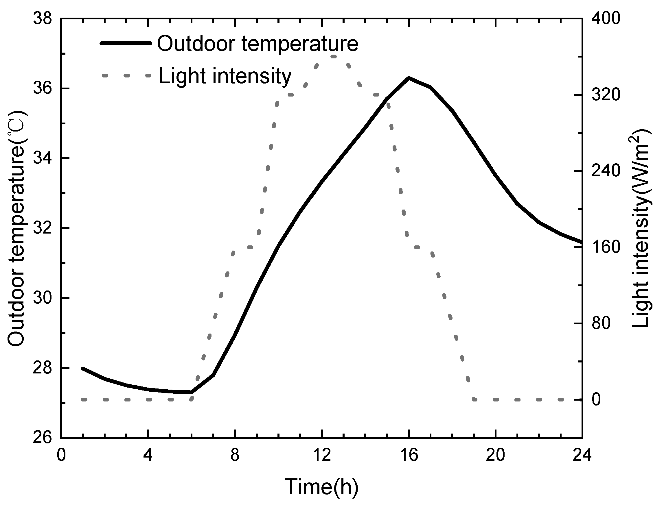
2.1. Analysis of Influencing Factors

In this paper, the influence factors of building room temperature change are analyzed by RC network model, and the input and output of the CNN room temperature calculation model are determined. Under a single refrigeration zone, the RC network model [8,9] is shown in Figure 3, and the mathematical model is shown in Equation (1). The R_wall in Figure 3 reflects the thermal insulation capacity of the walls in this room, while C_room and C_wall reflect the thermal storage capacity of the rooms and walls, respectively. T₁~T₄ are the temperatures of adjacent nodes in cooling zone i. If adjacent nodes are rooms, they are the temperatures of adjacent rooms. If the adjacent node is outdoors, it is the outdoor temperature. By connecting the units to each other, a model of a certain floor of the building can be formed. Figure 4 takes the topology of a certain layer of a building as 2 × 2 as an example to show the connection mode of each basic unit and the RC network model of a certain layer after connection. In Figure 4, T_o is the outdoor temperature.

$$\left\{\begin{array}{l}{C}_{\mathrm{room},\mathrm{i}}\frac{\mathrm{d}{T}_{\mathrm{room},\mathrm{i}}}{\mathrm{d}t}={\displaystyle \sum _{\mathrm{j}\in N_{\mathrm{wall},\mathrm{room},\mathrm{i}}^{}}\frac{T_{\mathrm{wall},\mathrm{i},\mathrm{j}}-T_{\mathrm{room},\mathrm{i}}}{R_{\mathrm{wall},\mathrm{i},\mathrm{j}}}+}{\pi }_{\mathrm{win},\mathrm{i},\mathrm{j}}^{}\times \\ {\displaystyle \sum _{\mathrm{j}\in N_{\mathrm{node},\mathrm{room},\mathrm{i}}^{}}\frac{T_{\mathrm{room},\mathrm{j}}-T_{\mathrm{room},\mathrm{i}}}{R_{\mathrm{win},\mathrm{i},\mathrm{j}}}+}{Q}_{\mathrm{int},i}-Q_{\mathrm{HVAC},i}+\tau A_{\mathrm{win},\mathrm{room},\mathrm{i}}{Q}_{\mathrm{rad},\mathrm{i}}\\ C_{\mathrm{wall},\mathrm{i},\mathrm{j}}\frac{\mathrm{d}{T}_{\mathrm{wall},\mathrm{i},\mathrm{j}}}{\mathrm{d}t}={\displaystyle \sum _{\mathrm{j}\in N_{\mathrm{wall},\mathrm{room},\mathrm{i}}^{}}\frac{T_{\mathrm{room},\mathrm{j}}-T_{\mathrm{wall},\mathrm{i},\mathrm{j}}}{R_{\mathrm{wall},\mathrm{i},\mathrm{j}}}+r_{\mathrm{i},\mathrm{j}}}{v}_{\mathrm{i},\mathrm{j}}{A}_{\mathrm{wall},\mathrm{i},\mathrm{j}}{Q}_{\mathrm{rad},\mathrm{i}}\end{array}\right.$$

(1)

where, C_room,i, T_room,i, Q_int,i, Q_HVAC,i, and A_win,room,i, respectively, represent the heat capacity, room temperature, internal heat production, central air conditioning cooling capacity, and window area of refrigeration area i. R_wall,i,j, C_wall,i,j, T_wall,i,j, and R_win,i,j are the thermal resistance, heat capacity, and temperature of the wall and the thermal resistance of the window between the i and j cooling zones, respectively; π_win,i,j, r_i,j, and τ are 0–1 variables; v_i,j is the heat absorption rate of the wall; N_wall,room,i and N_node,room,i are the sets of all walls and nodes connected to cooling zone i, respectively.

According to Equation (1), the temperature of each cooling area of the building depends on the heat production, cooling capacity, and outdoor temperature of the cooling area. Equation (1) is “encapsulated” and transformed, as shown in Equation (2).

$$\left\{\begin{array}{l}{Q}_{\mathrm{HVAC},t}^{}=f(T_{\mathrm{room},t}^{},\Delta T_{\mathrm{room},t+1}^{},T_{o,t}^{},Q_{\mathrm{heat},t}^{})\\ Q_{\mathrm{heat},t}^{}=Q_{\mathrm{rad},t}^{}+Q_{\mathrm{int},t}^{}\end{array}\right.$$

(2)

where, T_room,t and ΔT_room,t+1 are the temperature of all cooling zones at time t and the changing temperature of all cooling zones at time t + 1, respectively. T_o,t is the outdoor temperature at time t; Q_HVAC,t is the cooling capacity required by the building at time t; Q_heat,t is the heat gained by the building at time t; Q_rad,t and Q_int,t are the light intensity and the internal heat production of the building at time t.

From Equation (2), it can be seen that the cooling capacity required by the building at time t is related to the temperature T_room of each cooling area of the building at time t and the outdoor temperature to the Q_heat,t of the building and the temperature change ΔT_room,t+1 of each cooling area of the building at time t. Therefore, the building model based on CNN takes the independent variable in Equation (2) as input to model the cooling capacity Q_HVAC,t required to reach the target temperature.

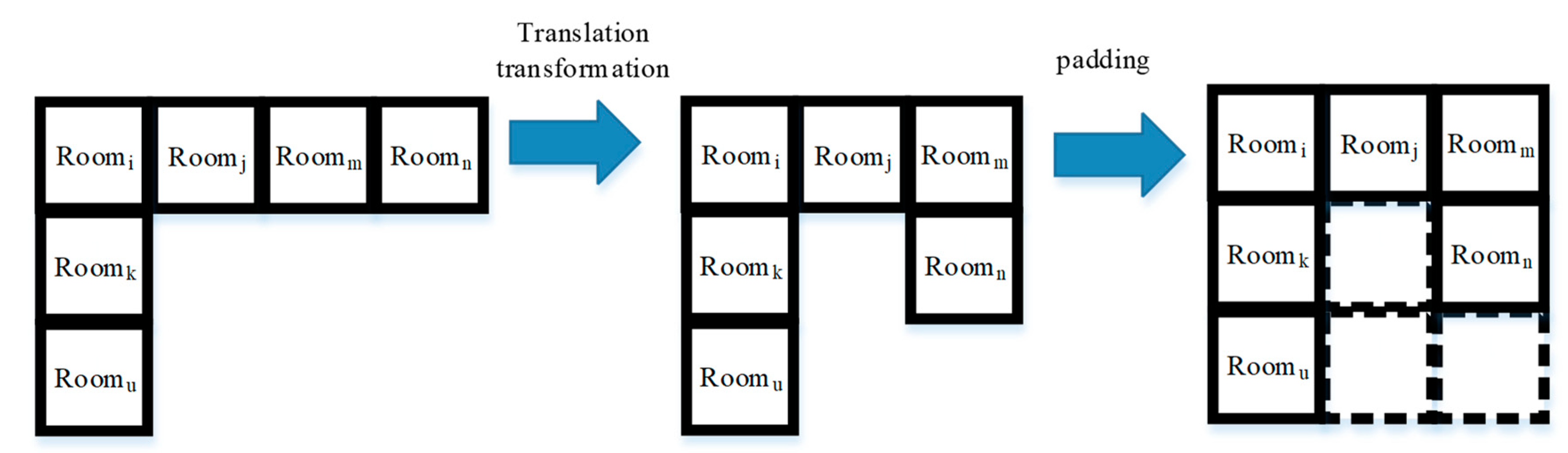
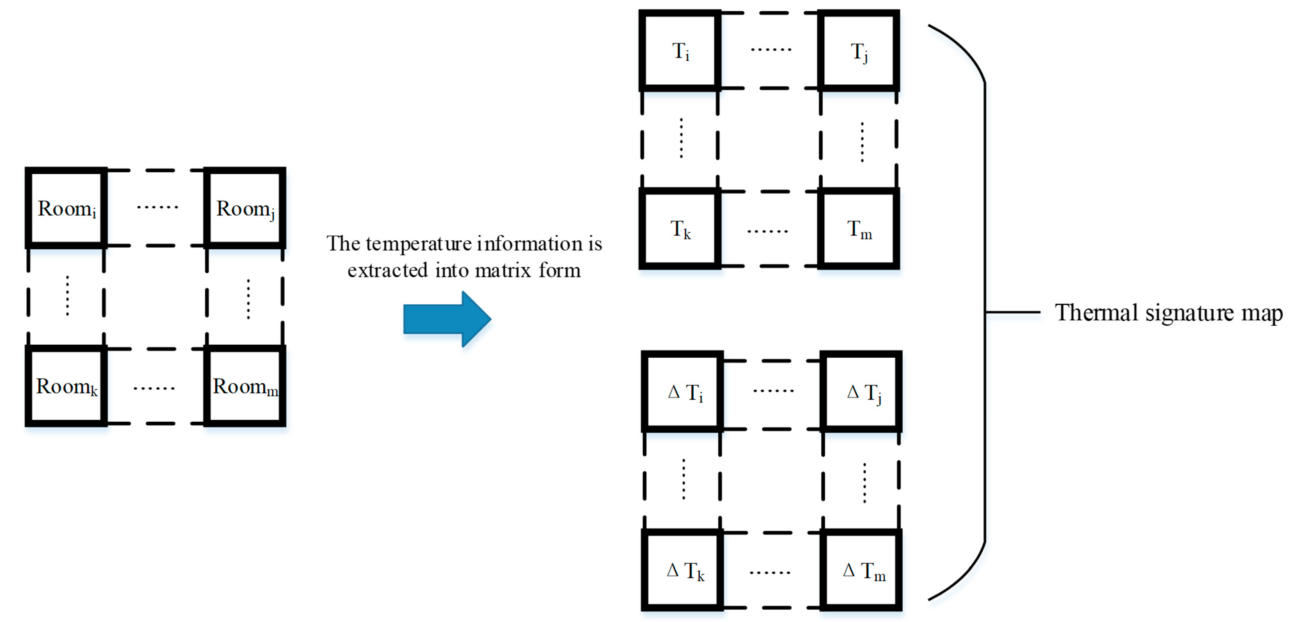
2.2. Network Structure Design

Convolutional operations are linear operations, and convolutional neural networks without activation functions are linear models. Therefore, the CNN building model proposed in this paper can be applied to linear programming. For a single-story building, the network structure is shown in Figure 5.

In the CNN building model, the temperature of each cooling area in the building and the target temperature change are made into a “thermal feature map”, and then, the CNN is used to carry out convolution operation on the “thermal feature map” and extract the feature. Considering that the cooling regions that are too far apart have little influence on each other, the convolution kernel size is set to 3 × 3 in this paper. A total of four convolution cores are set for each layer of convolution, and the convolution operation is repeated until the final feature is extracted. For the same building, there is no obvious difference between the outdoor temperature T_o,t and the light intensity Q_rad,t in each cooling area, so the outdoor temperature T_o,t and the light intensity Q_rad,t do not participate in the convolution operation but directly as the input of the fully connected layer.

For an n-story building, a total of 2n “thermal signature maps” are generated with 2n input channels. The network structure of CNN multi-story building model is shown in Figure 6.

3. Central Air Conditioning Energy Consumption Model and Its Optimal Working Condition

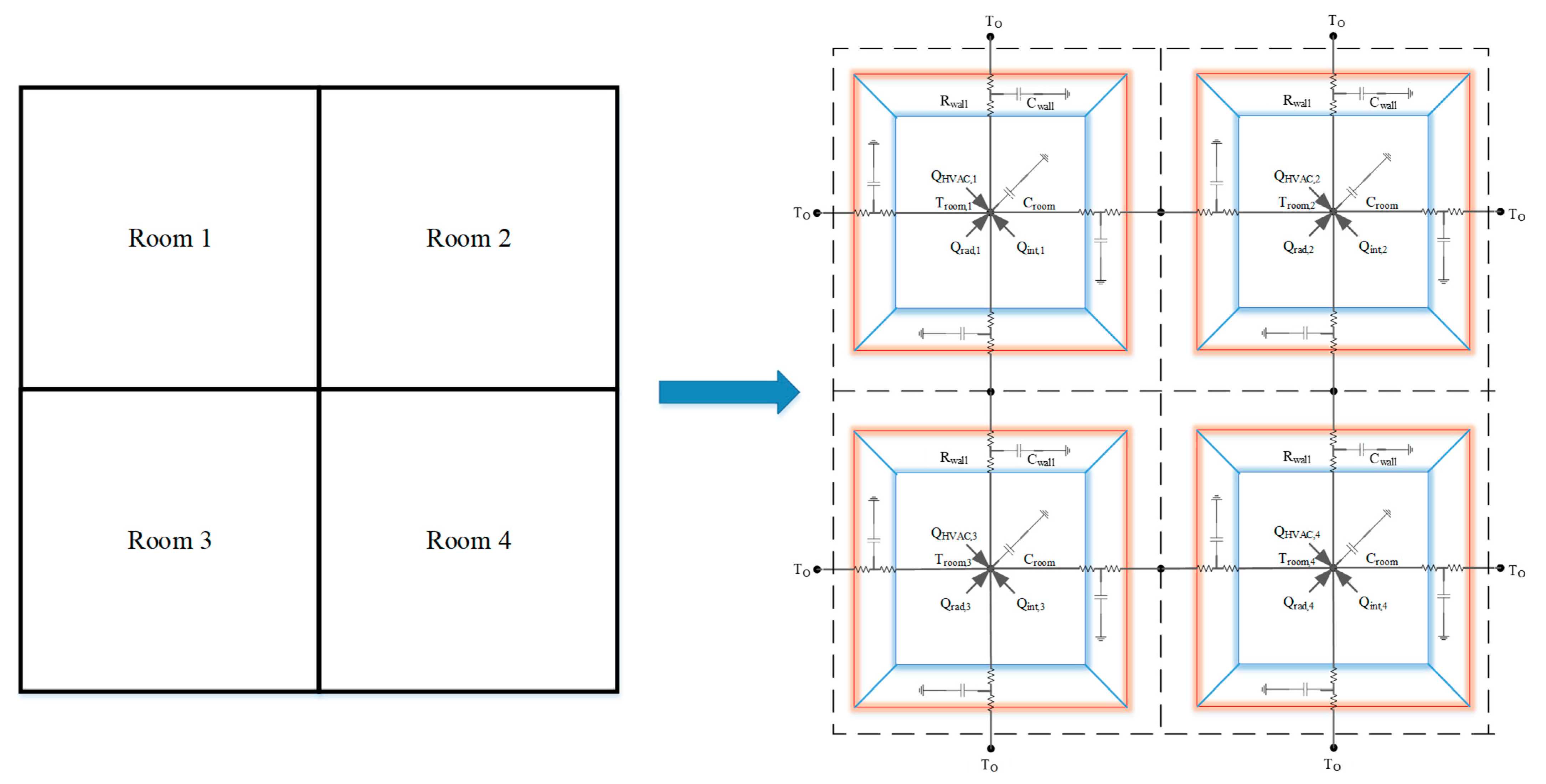
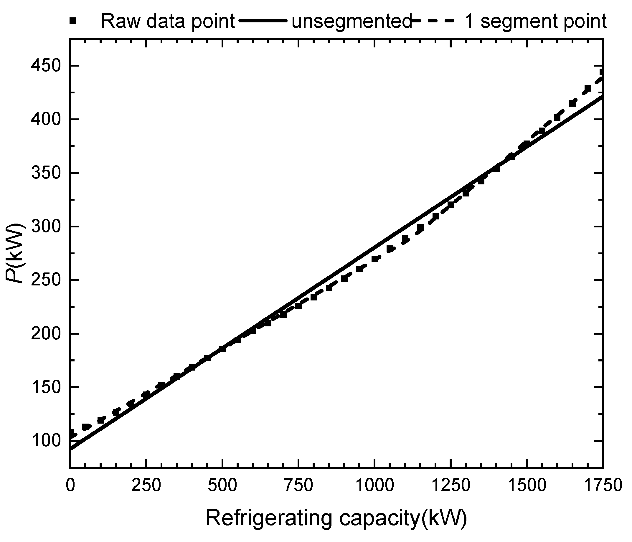
3.1. Energy Consumption Model

Central air conditioning is usually composed of a chilled water pump, cooling water pump, fan coil, cooling tower, and chiller, as shown in Figure 7.

The energy consumption of the chiller is shown in Equation (3).

$$PW{R}_{\mathrm{ch}}={\mathrm{a}}_0{+\mathrm{a}}_1(T_{\mathrm{cw},\mathrm{in}}-T_{\mathrm{chw},\mathrm{in}})+{\mathrm{a}}_2{(T_{\mathrm{cw},\mathrm{in}}-T_{\mathrm{chw},\mathrm{in}})}^2+{\mathrm{a}}_3(T_{\mathrm{cw},\mathrm{in}}-T_{\mathrm{chw},\mathrm{in}})Q_{\mathrm{e}}+{\mathrm{a}}_4{Q}_{\mathrm{e}}+{\mathrm{a}}_5{Q}_{\mathrm{e}}^2$$

(3)

where T_cw,in and T_chw,in are the temperature of cooling water and chilled water, respectively; a₀~a₅ are fitting coefficients; Q_e is the cooling capacity of the chiller.

The energy consumption models of the chilled water pump and cooling water pump are shown in Equations (4) and (5).

$$P_{\mathrm{eb}}={\mathrm{b}}_0+{\mathrm{b}}_1{G}_{\mathrm{e}}+{\mathrm{b}}_2{G}_{\mathrm{e}}^2$$

(4)

$$P_{\mathrm{cb}}={\mathrm{c}}_0+{\mathrm{c}}_1{G}_{\mathrm{c}}+{\mathrm{c}}_2{G}_{\mathrm{c}}^2$$

(5)

where G_e and G_c are the flow rate of the chilled water pump and the cooling water pump, respectively. b₀~b₂ and c₀~c₂ are fitting coefficients.

The fan coil energy consumption model is shown in Equation (6).

$$P_{\mathrm{k}}={\mathrm{d}}_0+{\mathrm{d}}_1{V}_{\mathrm{a}}+{\mathrm{d}}_2{V}_{\mathrm{a}}^2+{\mathrm{d}}_3{V}_{\mathrm{a}}^3$$

(6)

where V_a is the air volume of the fan coil; d₀~d₃ are fitting coefficients.

The cooling capacity generated by the fan coil is shown in Equation (7). The low-temperature chilled water in the coil is exchanged with the indoor heat through the fan blast.

$$Q_{\mathrm{t}}=Q_{\mathrm{t},0}\frac{T_{\mathrm{s}}-T_{\mathrm{chw},\mathrm{out}}}{T_{\mathrm{s}0}-T_{\mathrm{chw},\mathrm{out}0}}{\left(\frac{G_{\mathrm{e}}}{G_{\mathrm{e}0}}\right)}^{0.818}{\left(\frac{V_{\mathrm{a}}}{V_{\mathrm{a}0}}\right)}^{0.1912}$$

(7)

where T_s0, T_chw,out0, G_e0, V_a0, and Q_t,0, respectively, are the rated values of air inlet temperature, chilled water outlet temperature, chilled water flow rate, fan air volume, and cooling capacity under rated working conditions.

The energy consumption model of cooling tower fan is shown in Equation (8).

$$PW{R}_{\mathrm{f}}=PW{R}_{\mathrm{f},\mathrm{nom}}({\mathrm{e}}_0+{\mathrm{e}}_1(\frac{F_{\mathrm{a}}}{F_{\mathrm{a},\mathrm{nom}}})+{\mathrm{e}}_2{(\frac{F_{\mathrm{a}}}{F_{\mathrm{a},\mathrm{nom}}})}^2)$$

(8)

where PWR_f,nom, F_a, and F_a,nom are the rated energy consumption of the fan, the actual value of the fan air volume, and the rated value, respectively. e₀~e₂ are fitting coefficients.

The cooling tower transfers the heat in the cooling water to the outside through the built-in fan, and the corresponding cooling capacity is shown in Equation (9).

$$Q_{\mathrm{rej}}=\frac{{\mathrm{f}}_0{m}_{\mathrm{w}}^{{\mathrm{f}}_2}}{1+{\mathrm{f}}_1{(\frac{m_{\mathrm{w}}}{m_{\mathrm{a}}})}^{{\mathrm{f}}_2}}(T_{\mathrm{cw},\mathrm{out}}-T_{\mathrm{wb}})$$

(9)

where m_w and m_a are cooling water flow and fan flow, respectively; T_cw,out and T_wb are the cooling water outlet temperature and cooling tower air inlet temperature, respectively. f₀~f₂ are fitting coefficients.

Therefore, the total energy consumption of central air conditioning is shown in Equation (10).

$$P=PW{R}_{\mathrm{ch}}+P_{\mathrm{eb}}+P_{\mathrm{cb}}+P_{\mathrm{k}}+PW{R}_{\mathrm{f}}$$

(10)

3.2. Optimal Working Condition Solving Model

The cooling capacity of the central air conditioner is divided into N points on average from 0 to the rated value, and the sum of the energy consumption of all points is the minimum as the objective function, as shown in Equation (11).

$$\left\{\begin{array}{l}\min {\displaystyle \sum _{i=1}^N{P}_{\mathrm{i}}}(Q_i)\\ Q_{\mathrm{i}}=\frac{i}{N}{Q}_{\mathrm{n}}\end{array}\right.$$

(11)

Constraints include working condition constraints and thermodynamic constraints, as shown in Equations (12) and (13).

With Equation (11) as the goal and Equations (12) and (13) as the constraint, the minimum energy consumption under each cooling capacity is obtained, and then, the “cooling capacity minimum energy consumption” curve is segmented and linearized to obtain the linearized energy consumption model of central air conditioning.

$$\left\{\begin{array}{l}{Q}_{\mathrm{emin}}\le Q_{\mathrm{e},\mathrm{i}}\le Q_{\mathrm{emax}}\\ G_{\mathrm{emin}}\le G_{\mathrm{e},\mathrm{i}}\le G_{\mathrm{emax}}\\ G_{\mathrm{cmin}}\le G_{\mathrm{c},\mathrm{i}}\le G_{\mathrm{cmax}}\\ F_{\mathrm{amin}}\le F_{\mathrm{a},\mathrm{i}}\le F_{\mathrm{amax}}\\ V_{\mathrm{amin}}\le V_{\mathrm{a},\mathrm{i}}\le V_{\mathrm{amax}}\\ T_{\mathrm{chw},\mathrm{in},\min }\le T_{\mathrm{chw},\mathrm{i},\mathrm{in}}\le T_{\mathrm{chw},\mathrm{in},\max }\\ T_{\mathrm{cw},\mathrm{in},\min }\le T_{\mathrm{cw},\mathrm{i},\mathrm{in}}\le T_{\mathrm{cw},\mathrm{in},\max }\end{array}\right.$$

(12)

$$\left\{\begin{array}{l}{Q}_{t,\mathrm{i}}=Q_{\mathrm{e},\mathrm{i}}=Q_{\mathrm{i}}\\ Q_{\mathrm{rej},\mathrm{i}}=Q_{\mathrm{e},\mathrm{i}}+PW{R}_{\mathrm{ch},\mathrm{i}}\\ T_{\mathrm{chw},\mathrm{i},\mathrm{in}}-T_{\mathrm{chw},\mathrm{i},\mathrm{out}}=\frac{3600Q_{\mathrm{e},\mathrm{i}}}{1000C{G}_{\mathrm{e},\mathrm{i}}}\\ T_{\mathrm{cw},\mathrm{i},\mathrm{out}}-T_{\mathrm{cw},\mathrm{i},\mathrm{in}}=\frac{3600Q_{\mathrm{e},\mathrm{i}}}{1000C{G}_{\mathrm{c},\mathrm{i}}}\end{array}\right.$$

(13)

4. Load-Shedding Potential and Economic Load-Shedding Strategy of Central Air Conditioning Cluster

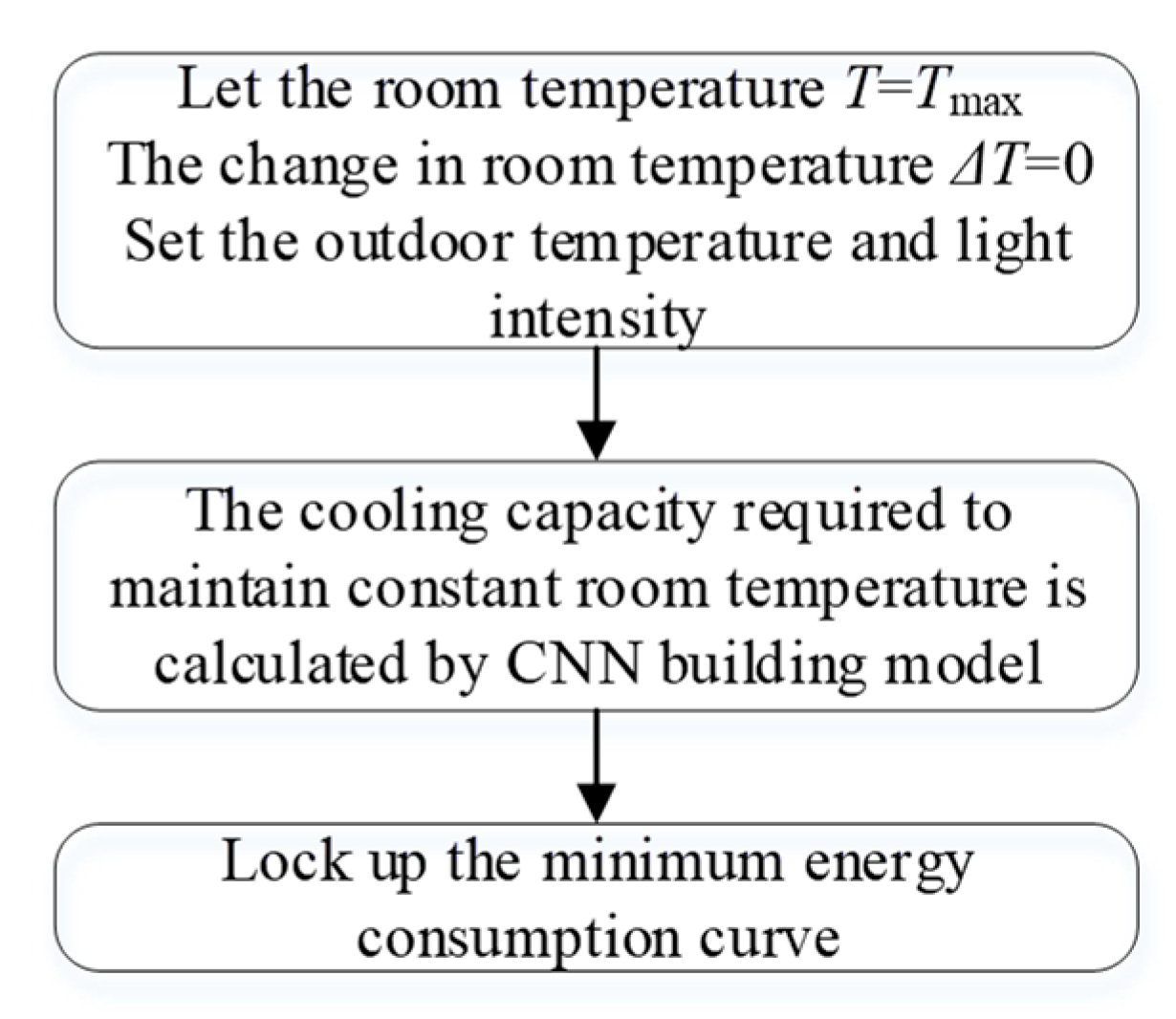
4.1. Load Baseline Calculation Method

In order to evaluate the load-reduction potential of the central air conditioning cluster, the central air conditioning load baseline should be calculated first. The load baseline is calculated based on the CNN building model and minimum energy consumption curve proposed in the paper, and the calculation process is shown in Figure 8.

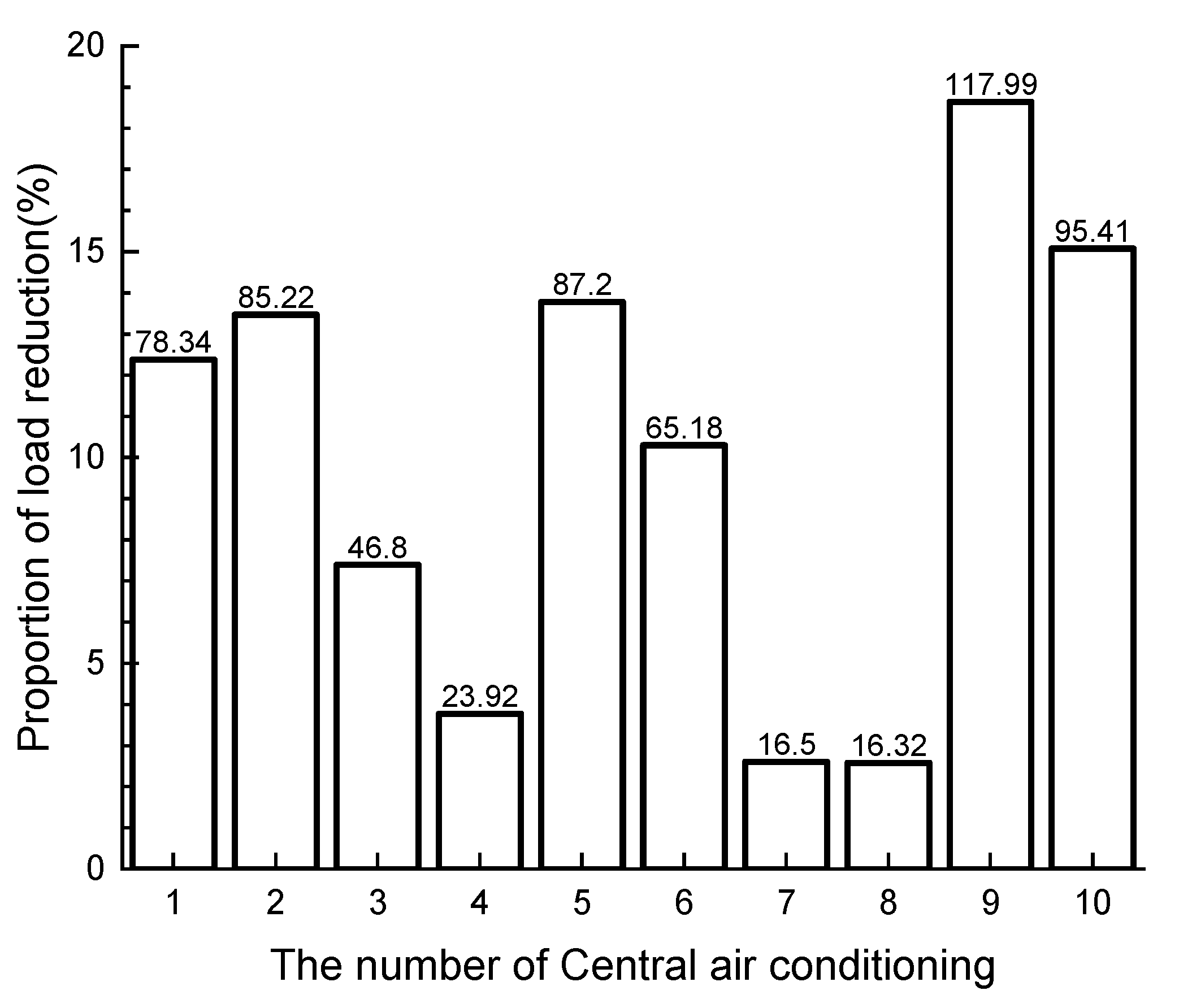
4.2. Load Reduction Potential Evaluation Model

The building has the characteristics of heat storage, and the central air conditioning has the minimum startup energy consumption, so the central air conditioning cluster can reduce the load during the demand-response period based on advance cooling and alternate start and stop.

The minimum energy consumption of the central air conditioning cluster during the demand-response period is taken as the objective function, as shown in Equation (14).

$$\min {\displaystyle \sum _{i=1}^N{\displaystyle \sum _{t\in \tau }{P}_t^{\prime i}(Q_{\mathrm{e},t}^i)}}$$

(14)

where N is the number of units; τ is the demand-response period.

The constraints include comfort constraints, stability constraints of load-reduction value, cooling capacity constraints, and additional constraints of model linearization, as shown in Equation (15).

$$\left\{\begin{array}{l}{T}_{\min }\le T_{\mathrm{room},\mathrm{i},t}\le T_{\max }\\ P_{\mathrm{n},\mathrm{i}}^{}-P_{\mathrm{i}}^{\prime }(Q_{\mathrm{e},\mathrm{i}})=P_{\mathrm{n},\mathrm{k}}^{}-P_{\mathrm{k}}^{\prime }(Q_{\mathrm{e},\mathrm{k}}),\mathrm{i},\mathrm{k}\in \tau \\ s_{t,\mathrm{i}}{Q}_{\mathrm{emin}}\le Q_{\mathrm{e},t,\mathrm{i}}\le s_{t,\mathrm{i}}{Q}_{\mathrm{emax}}\\ P_{t,\mathrm{i}}^{\prime }(Q_{\mathrm{e},t,\mathrm{i}})\ge k{Q}_{\mathrm{e},t,\mathrm{i}}+b{s}_{t,\mathrm{i}}\\ P_{t,\mathrm{i}}^{\prime }(Q_{\mathrm{e},t})\le k{Q}_{\mathrm{e},t,\mathrm{i}}+b+M(1-s_{t,\mathrm{i}})\\ 0\le P_{t,\mathrm{i}}^{\prime }(Q_{\mathrm{e},t,\mathrm{i}})\le s_{t,\mathrm{i}}{P}_{\mathrm{e},\max }\end{array}\right.$$

(15)

where s_t,i is the on–off state of unit i at time t; k and b are the linearization coefficients of the minimum energy consumption curve. M is some great positive number; P_n,i indicates the baseline load value of the central air conditioner cluster during period i.

Without the last three equations in Equation (15), the system energy consumption is calculated directly by the product of the on–off state and the power of the central air conditioning unit, which will introduce nonlinearity into the objective function and cause the problem to be difficult to solve.

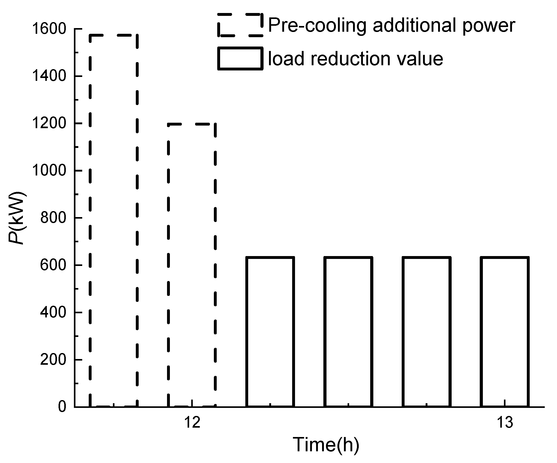
4.3. Economic Load Reduction Strategy

Under the given load-reduction capacity, the energy consumption of the central air conditioning cluster in the demand-response period is determined by the load-reduction capacity and cannot be regulated. Therefore, the economic load-reduction strategy takes the minimum energy consumption during the advance cooling period as its objective function, as shown in Equation (16).

$$\min {\displaystyle \sum _{i=1}^N{\displaystyle \sum _{t\in \lambda }{P}_t^{\prime i}(Q_{\mathrm{e},t}^i)}}$$

(16)

where λ is the advance cooling period.

The constraint conditions still include comfort constraint, cooling capacity constraint, load-reduction value constraint, and additional model linearization constraint, as shown in Equation (17). Since the maximum load-reduction potential is evaluated before the economic load-reduction strategy is formulated, the equation constraint on the load-reduction value can still ensure the solvability of the optimization problem.

$$\left\{\begin{array}{l}{T}_{\min }\le T_{\mathrm{room},\mathrm{i},t}\le T_{\max }\\ P_{n,t}^{}-P_t^{\prime }(Q_{e,t})=K_{cp}{P}_{cp,\max }, \mathrm{i},\mathrm{k}\in \tau \\ s_{t,\mathrm{i}}{Q}_{\mathrm{emin}}\le Q_{\mathrm{e},t,\mathrm{i}}\le s_{t,\mathrm{i}}{Q}_{\mathrm{emax}}\\ P_{t,\mathrm{i}}^{\prime }(Q_{\mathrm{e},t,\mathrm{i}})\ge k{Q}_{\mathrm{e},t,\mathrm{i}}+b{s}_{t,\mathrm{i}}\\ P_{t,\mathrm{i}}^{\prime }(Q_{\mathrm{e},t})\le k{Q}_{\mathrm{e},t,\mathrm{i}}+b+M(1-s_{t,\mathrm{i}})\\ 0\le P_{t,\mathrm{i}}^{\prime }(Q_{\mathrm{e},t,\mathrm{i}})\le s_{t,\mathrm{i}}{P}_{\mathrm{e},\max }\end{array}\right.$$

(17)

where K_cp is the load-reduction ratio, which is 0~1; P_cp,max is the maximum load-reduction value, which can be calculated by the evaluation model in Section 4.2.

5. Example Analysis

5.1. CNN Building Model

5.1.1. Data Set Design

In this paper, a discrete RC network model is used to generate the training data required by the CNN building model. The simulation step size is 1s, and the period is 15 min. The building topology is set to single-layer 5 × 5. A total of 10 buildings are set in the example, and the 10 building parameters are shown in

Table 2. Building parameters and comfort range of each building.

Building Number	Wall Thermal Resistance Rwall (K/W)	Thermal Resistance of Windows Rwin (K/W)	Wall Heat Capacity Cwall (J/K)	Room Heat Capacity Croom (J/K)	Comfort Range (°C)
1	0.08	0.02	2.6 × 107	2.5 × 105	20~25
2	0.12	0.03	2.6 × 107	2.5 × 105	20~25
3	0.06	0.015	2.6 × 107	2.5 × 105	20~25
4	0.04	0.1	2.6 × 107	2.5 × 105	20~25
5	0.08	0.02	3.9 × 107	3.75 × 105	20~25
6	0.08	0.02	1.95 × 107	1.875 × 105	20~25
7	0.08	0.02	1.3 × 107	1.25 × 105	20~25
8	0.08	0.02	2.6 × 107	2.5 × 105	21~24
9	0.08	0.02	2.6 × 107	2.5 × 105	19~26
10	0.08	0.02	2.6 × 107	2.5 × 105	18~27

.

In order to ensure the training effect of CNN, training samples should be spread across all possible data points as far as possible. This paper generates samples by randomly sampling within the range of parameter variation. The variation range of each parameter is shown in

Table 3. The range of variation of the relevant parameters of the data set.

Argument	Range
Room temperature initial value Troom,i (°C)	Tmin~Tmax
Light intensity Qrad (W)	0~360
Outdoor temperature To (°C)	26~38
Cooling capacity per cooling area QHVAC,t (W)	0~1500

.

As can be seen from Table 3, the input values of the neural network differ greatly. In order to speed up the training of the neural network and avoid falling into the local optimal solution, the data set can be normalized, as shown in Equation (18).

$$x^{\prime }=\frac{x-\min (x)}{\max (x)-\min (x)}$$

(18)

where x represents the data before normalization.

5.1.2. Training Effect

This paper uses root mean squared error (RMSE) and accuracy to reflect the training effect of CNN building model, as shown in Equations (19) and (20).

$$RMSE=\sqrt{\frac{1}{n}{\displaystyle \sum _{i=1}^n{(y_i-y_{hat,i})}^2}}$$

(19)

$$Acc=1-\frac{1}{n}{\displaystyle \sum _{i=1}^n\frac{\left|y_i-y_{hat,i}\right|}{y_i}}$$

(20)

where y_i is the true value of the data set, corresponding to the Q_HVAC of the article; y_hat,i is the predicted value, corresponding to the CNN building model output.

Based on Pytorch, the CNN building model is trained using GPU, and the learning rate is set to 0.3. Taking building 1 as an example, the training effect is shown in

Table 4. The training effect of the building thermal model based on CNN.

Training Times	Loss	RMSE	Acc
1	355,408,544	18,852.28	0.1345%
2	352,316,576	18,770.09	0.5724%
3	345,913,856	18,598.75	1.484%
……	……	……	……
99,998	1432.64	37.85	99.83%
99,999	1432.13	37.84	99.84%
100,000	1432.07	37.84	99.84%

.

As can be seen from Table 4, the CNN building model proposed in the paper can accurately model the cooling capacity Q_HVAC required by the building, and the accuracy rate can reach 99.84% after 100,000 training sessions.

Compared with the ETP model and RC network model, the improvement effect of the CNN building model is shown in

Table 5. Comparison table of improved effect between the CNN-based building thermal model and traditional model.

Model	Calculation Time	Parameter Number	The Number of Measurement Points Required to Identify the Model	Whether Interaction Can Be Considered
ETP model	Negligible	4	1	×
RC model	1.053 s	145	85	√
CNN model	0.189 s	81	25	√

.

The identification of RC model requires the measurement of the temperature of each wall and cooling area, and the number of measurement points is quite large. The CNN building model can only measure the temperature of the cooling area, and the influence of the wall temperature on the room temperature is reflected in the historical data. Compared with the ETP model, the CNN building model proposed in this paper solves the technical drawback of not being able to consider the temperature difference and interaction in the cooling zone. Compared with the RC network model, the calculation speed is increased, and the number of measurement points required for model identification is reduced.

5.2. Optimal Condition of Central Air Conditioning

This paper uses the model parameters of central air conditioning provided in the literature [14]. Each building is equipped with eight end fan coils, one cooling water pump, one freezing water pump, one chiller, and one cooling tower. With Equation (11) as the objective function and Equations (12) and (13) as the constraint conditions, the minimum energy consumption curve of the central air conditioning under each cooling capacity is solved and segmented and linearized, as shown in Figure 9. It can be seen that the minimum power consumption of the central air conditioning system in the paper is about 107.93 kW, accounting for about 24.30% of the maximum energy consumption.

In addition to the chiller, the energy consumption of other components under optimal working conditions and their accounts are shown in Figure 10. It can be seen that even under the optimal working conditions, the energy consumption of the remaining components is about 22% to 34%. Therefore, the central air conditioner is different from the split air conditioner, and only considering the energy consumption of the chiller will bring a large error.

5.3. Load-Reduction Potential Evaluation and Economic Load-Reduction Strategy

5.3.1. Load Base Line

Before assessing the load-reduction potential, the load baseline needs to be calculated.

In the calculation example, the 24 h outdoor temperature and light intensity curve is shown in Figure 11.

The load baseline of 10 building examples is calculated according to the process shown in Figure 8, and the results are shown in Figure 12.

5.3.2. Load-Reduction Potential Assessment

In this paper, the pre-cooling period is from 11:30 to 12:00, and the demand-response load-reduction period is from 12:00 to 13:00. With Equation (14) as the objective function and (15) as the constraint condition, Cplex is used to evaluate the maximum load-reduction potential of 10 building examples. By calculation, the maximum load-reduction potential of the building example in article 10 is 632.87 kW, accounting for about 31.06% of the load baseline in the corresponding period.

Pre-cooling will make the central air conditioning energy consumption greater than the load base, the power consumed by pre-cooling is the additional power of pre-cooling, and the value of pre-cooling additional power and load reduction is shown in Figure 13.

The ratio of power reduction of each unit to total power reduction during the demand-response period reflects the contribution of each unit in load reduction. Figure 14 shows the contribution of each unit in load reduction under the maximum load-reduction potential. The thermal resistance of a building reflects the heat-insulation capacity of a building, and the heat capacity of a building reflects the heat-storage capacity of a building. Buildings 4 and 7 have low load-reduction output due to low thermal resistance and heat capacity. The comfort range affects the flexibility and adjustable depth of the operation of the central air conditioning in the building. The comfort range of building 8 is narrow, and its load-reduction potential is low.

Under the maximum load-reduction potential, the average room temperature change of each building is shown in Figure 15. It can be seen that all buildings have different degrees of advance cooling, and at the end of the demand-response period, the room temperature rises back to the comfort limit, meaning that the cold stored in pre-cooling is released.

The energy consumption of each central air conditioning unit is shown in Figure 16. It can be seen that except for units 4, 7, and 8, the rest of the units are alternately started and stopped during the load-reduction period. Due to the low thermal resistance and heat capacity of buildings 4 and 7 (small thermal inertia), the comfort range of building 8 is narrow, and a shutdown of 15 min will cause the room temperature of these buildings to exceed the comfort limit, so it will not participate in the alternate start and stop.

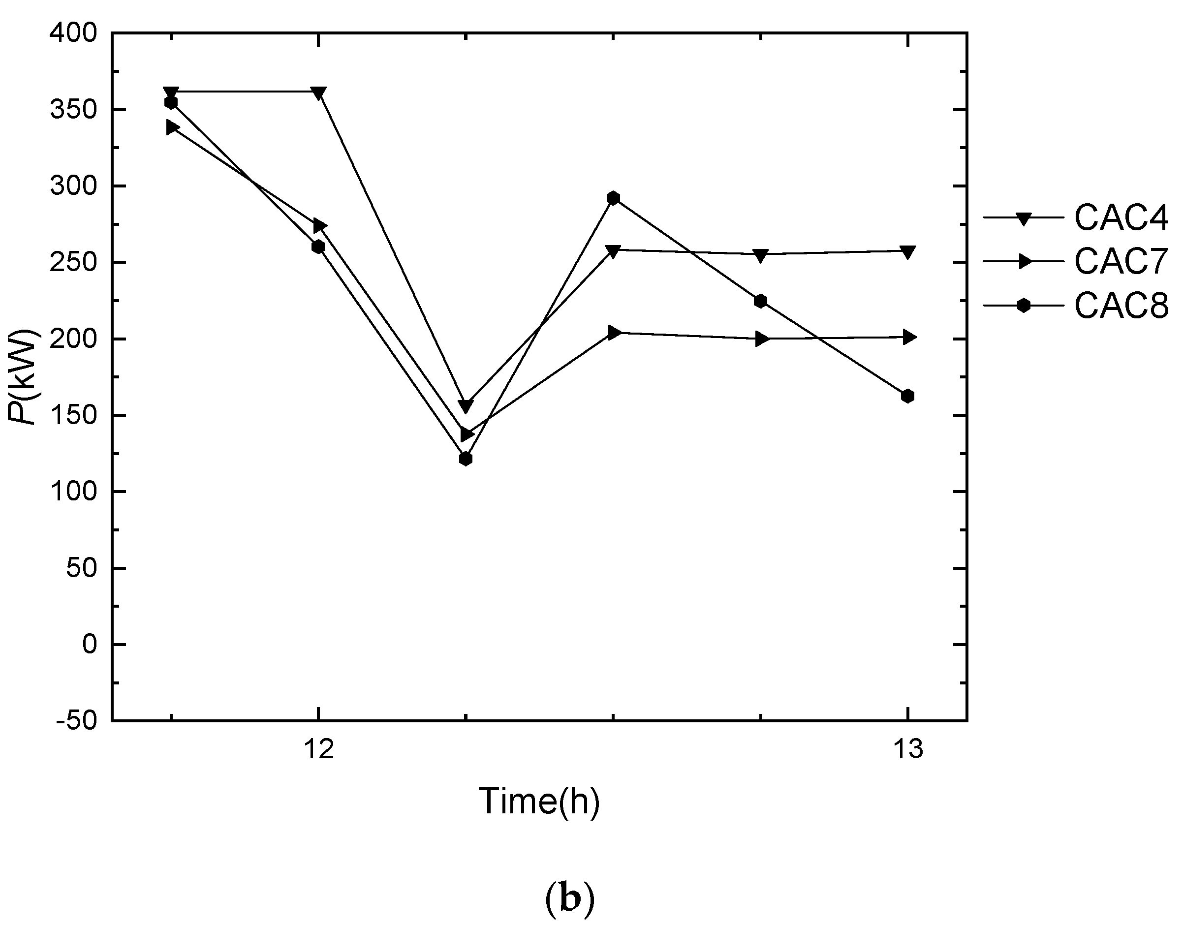
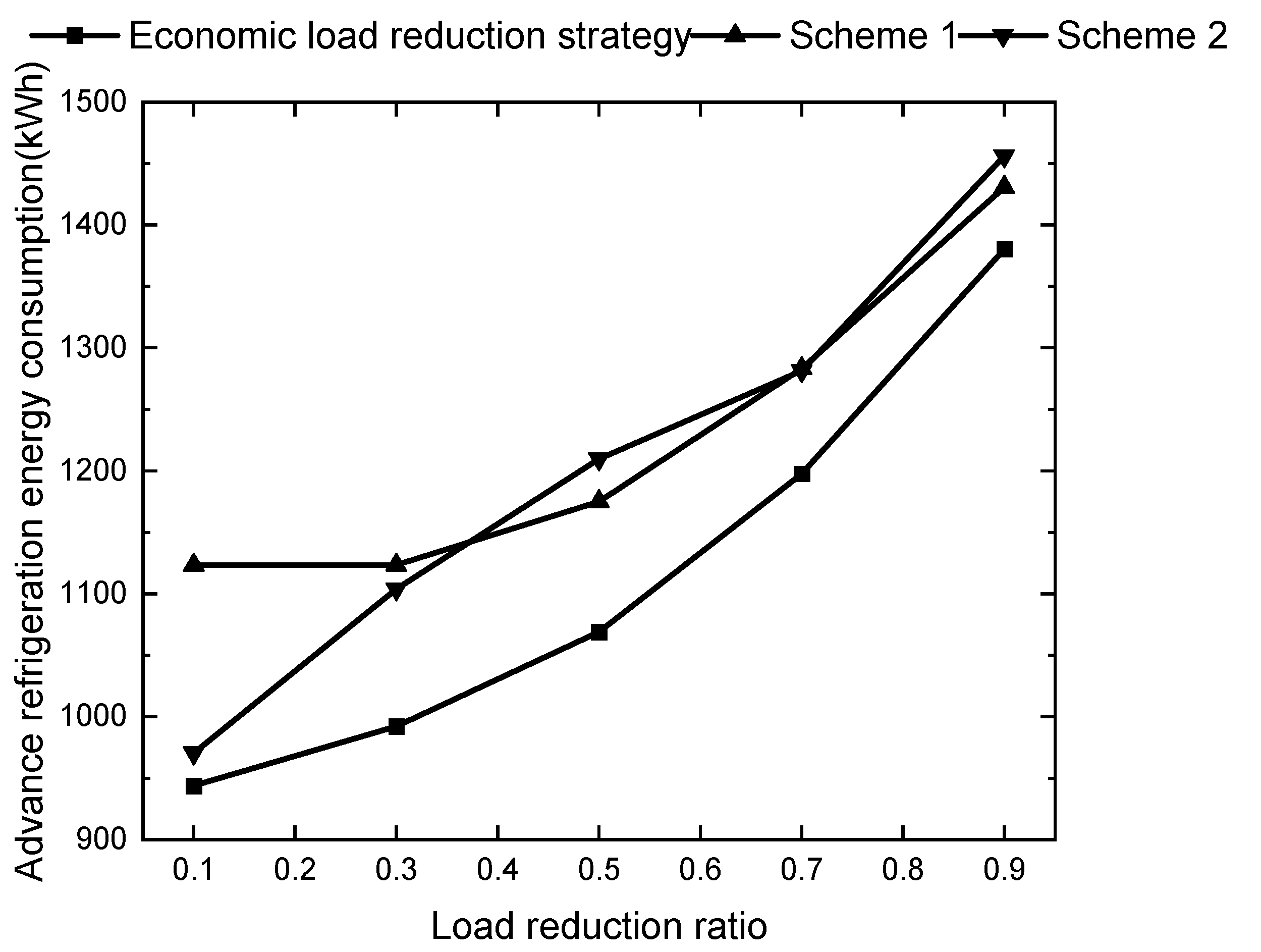
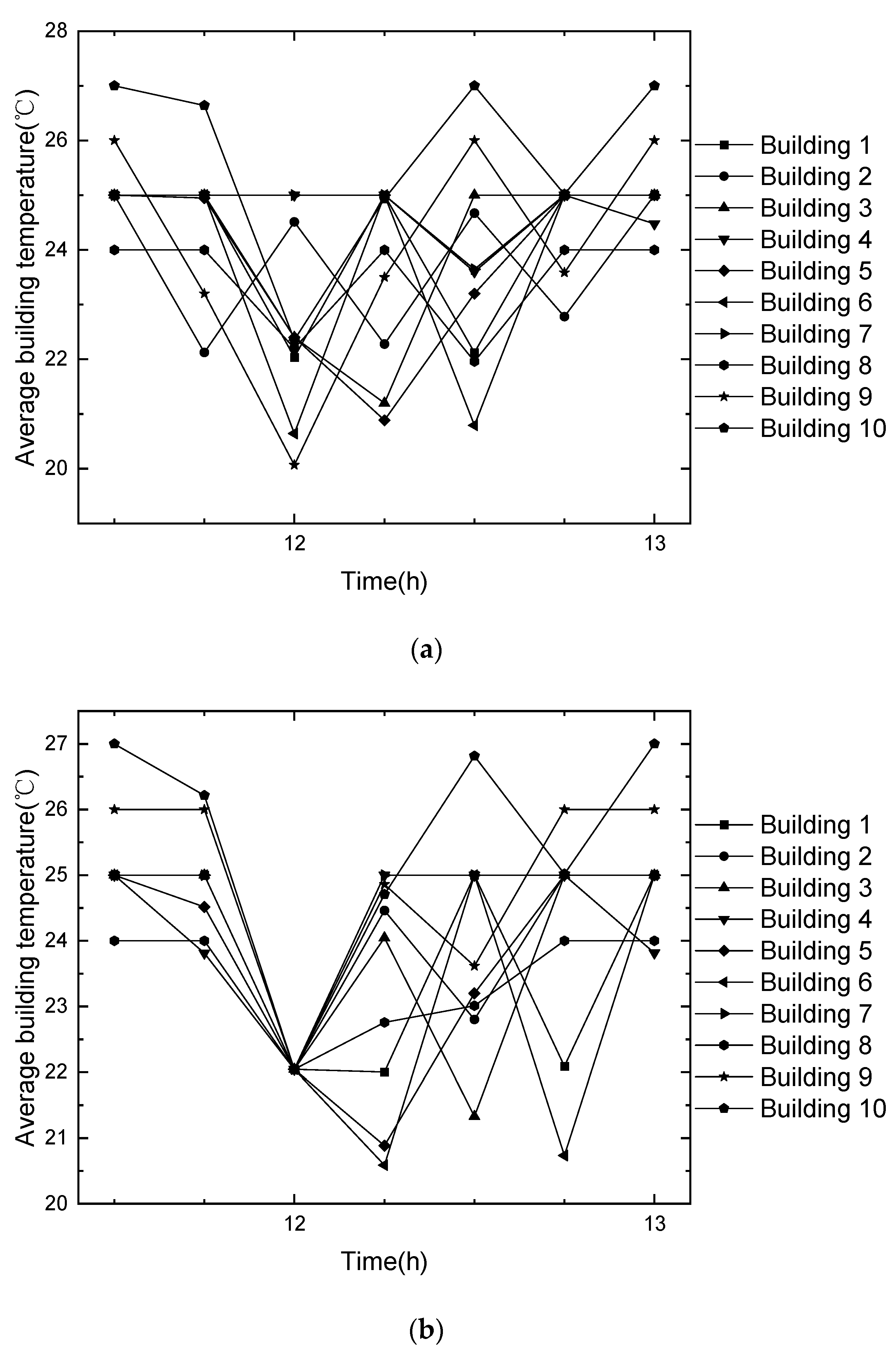
5.3.3. Economic Load-Reduction Strategy

After evaluating the maximum load-reduction potential of the central air conditioning cluster, using Equation (16) as the objective function and Equation (17) as the constraint condition, Cplex can be used to solve the economic load-reduction operation mode under each load-reduction ratio.

In order to show the economy of the strategy proposed in this paper, the following two conventional advance cooling schemes are formulated:

Scheme 1: All buildings are cooled to the same temperature in advance. If the target load-reduction value is large, cooling to the same temperature cannot complete the load-reduction target, and it is not required that buildings 8 to 10 (comfort range is different from other buildings) maintain the same temperature.

Scheme 2: The relative value of pre-cooling of each building is equal. For example, buildings 1~7 are pre-cooled to 21 °C, decreasing 4 °C and accounting for 80% of the comfort range; building 8 is pre-cooled to 21.6 °C, decreasing 2.4 °C and accounting for 80% of the comfort range.

Under a different load-reduction ratio, i.e., K_cp, the pre-cooling energy consumption of two conventional load-reduction strategies and economic load-reduction strategies is shown in Figure 17. It can be seen that scheme 2 is better than scheme 1 under the low load-reduction coefficient. Under high load-reduction coefficient, scheme 1 is slightly better than scheme 2. The economic load-reduction strategy is generally superior to scheme 1 and scheme 2. Compared with scheme 1, the economic load-reduction strategy can save up to 179.65 kWh of electric energy, which is about 17.89% of the load baseline energy consumption. Up to 140.70 kWh of electricity is saved compared with option 2, which is about 14.01% of the load baseline energy consumption. In China, the electricity price of commercial buildings at noon is 1.2 RMB/kWh. Compared with scheme 1 and scheme 2, the economic load-reduction strategy saves at most RMB 215.58 and RMB 168.84, respectively.

Taking the load-reduction ratio of 0.2 and 0.8 as an example, the total load curve of the economic load-reduction strategy and the two conventional load-reduction schemes is shown in Figure 18. In the figure, 12:00 to 13:00 is the load-reduction period, and the energy consumption of the central air conditioning cluster during this period is determined by the target load-reduction value (or target load-reduction ratio) independent of the pre-cooling scheme adopted. Therefore, the load curves of the economic load-reduction strategy and the two conventional load-reduction schemes overlap during the 12:00 to 13:00 period. The pre-cooling period is 11:30 to 12:00, and the energy consumption in this period is determined by the pre-cooling scheme.

When the load-reduction ratio is 0.2, the pre-cooling energy consumption and cost of the economic load-reduction strategy and the two conventional load-reduction strategies are shown in

Table 6. When the load-reduction ratio is 0.2, the pre-cooling energy consumption and cost are compared between the economic load-reduction strategy and two conventional load-reduction strategies.

Scheme	Pre-Cooling Energy Consumption (kWh)	Cost (RMB)
Economic load-reduction strategy	959.29	1151.15
Conventional scheme 1	1123.54	1348.25
Conventional scheme 2	1043.89	1252.67

. The results for when the load-reduction ratio is 0.8 are shown in

Table 7. When the load reduction ratio is 0.8, the pre-cooling energy consumption and cost are compared between the economic load-reduction strategy and two conventional load reduction strategies.

Scheme	Pre-Cooling Energy Consumption (kWh)	Cost (RMB)
Economic load-reduction strategy	1287.08	1544.49
Conventional scheme 1	1365.27	1638.32
Conventional scheme 2	1365.62	1638.74

.

Through simulation verification, both the economic load-reduction strategy proposed in this paper and the two conventional strategies can meet the requirements for comfort. Taking the load-reduction ratio of 0.8 as an example, the average room temperature change of the three schemes is shown in Figure 19.

6. Conclusions

In order to alleviate the technical drawbacks of existing building models, this paper first proposes a building model based on CNN. Compared with the ETP model, this model can take into account the temperature difference and interaction between different cooling areas of the building. Compared with RC network model, the calculation speed is increased, and the number of measurement points required for model identification is reduced. Taking the single-layer 5 × 5 building topology as an example, the training of CNN building model is completed. Then, the energy consumption model and optimal working condition solution model of central air conditioning are established, which lays a foundation for the load-reduction strategy of central air conditioning. Finally, on the basis of the modeling work in this paper, the load-reduction potential evaluation method and economic load-reduction strategy of the central air conditioning cluster based on advance cooling and alternate start and stop are proposed.

The simulation results show the following: (1) The minimum startup energy consumption of the central air conditioning unit still accounts for about 24.30% of the rated energy consumption under the optimal working condition. In addition to the chiller, the remaining components of the central air conditioning system account for about 22% to 34% of energy consumption. (2) In the case of the 10 buildings in the paper, the maximum load-reduction potential of the central air conditioning cluster based on advance cooling and alternate start–stop is 632.87 kW, accounting for 31.06% of the load baseline in the corresponding period. (3) Compared with the two conventional load-reduction strategies, the economic load-reduction strategy proposed in this paper significantly improves the economy, saving up to 179.65 kWh and 140.70 kWh of electric energy, respectively, accounting for 17.89% and 14.01% of the baseline load energy consumption.

References

1. Song, M.; Gao, C.; Su, W. Modeling and controlling of air-conditioning load for demand response applications. Dianli Xitong Zidonghua/Autom. Electr. Power Syst. 2016, 40, 158–167. [Google Scholar] [CrossRef]
2. Bao, Y.; Cheng, L. Parameter identification method of second-order equivalent thermal parameter model for air conditioning loads. Autom. Electr. Power Syst. 2021, 45, 37–43. [Google Scholar]
3. Wu, C.; Shen, H.; Wang, Z. Data-driven online identification method for parameters of inverter air-conditioning load model. Autom. Electr. Power Syst. 2022, 46, 120–129. [Google Scholar]
4. Liao, S.; Xu, J.; Jin, C. Modeling and optimization for home appliances based on air-conditioning parameters identification. Electr. Meas. Instrum. 2019, 56, 43–47+68. [Google Scholar]
5. Lu, T. Research on Energy Storage Modeling and Control Strategy of the Air Conditioning Load; Southeast University: New Albany, Indiana, 2015. [Google Scholar]
6. Wang, C.; Fu, S.; Zhang, L.; Jiang, Y.; Shu, Y. Optimal control of source–load–storage energy in DC microgrid based on the virtual energy storage system. Energy Rep. 2023, 9, 621–630. [Google Scholar] [CrossRef]
7. Tu, C.; Cao, J.; Yu, D. Control strategy of virtual energy storage system participating in frequency modulation based on air conditioning loads. Power Demand Side Manag. 2019, 21, 16–21. [Google Scholar]
8. Chen, H.; Li, Z.; Jin, X.; Jiang, T.; Li, X.; Mu, Y. Modeling and Optimization of Active Distribution Network With Integrated Smart Buildings. Zhongguo Dianji Gongcheng Xuebao/Proc. Chin. Soc. Electr. Eng. 2018, 38, 6550–6562. [Google Scholar] [CrossRef]
9. Chen, H.; Li, Z.; Jang, T. Flexible energy scheduling strategy in smart buildings based on model predictive control. Autom. Electr. Power Syst. 2019, 43, 116–124. [Google Scholar]
10. Fan, D.; Zhang, Z.; Wang, Y. Day ahead scheduling strategy for air conditioning load aggregators considering user regulation behavior diversity. Power Syst. Prot. Control 2022, 50, 133–142. [Google Scholar]
11. Yang, X.; Fu, G.; Liu, F. Potential evaluation and control strategy of air conditioning load aggregation response considering multiple factors. Power Syst. Technol. 2022, 46, 699–714. [Google Scholar]
12. Yang, X.; Ding, X.; Lu, X. Inverter air conditioner load modeling and operational control for demand response. Power Syst. Prot. Control 2021, 49, 132–140. [Google Scholar]
13. Yang, J.; Shi, K.; Cui, X. Peak load reduction method of inverter air-conditioning group under demand response. Autom. Electr. Power Syst. 2018, 42, 44–52. [Google Scholar]
14. Pan, L.; Wang, S.; Wang, J.; Xiao, M.; Tan, Z. Research on Central Air Conditioning Systems and an Intelligent Prediction Model of Building Energy Load. Energies 2022, 15, 9295. [Google Scholar] [CrossRef]
15. Zhang, Q. Study on Energy Saving Control Strategies of Central Air Conditioning System; Southeast University: New Albany, Indiana, 2016. [Google Scholar]
16. Li, H. Optimization Control and Energy Saving Technology for Cooling System of HVAC System; Xi’an University of Architecture and Technology: Xi’an, China, 2011. [Google Scholar]
17. Jiang, i.; Ju, P.; Wang, C.; Li, H.; Liu, J. Coordinated Control of Air-Conditioning Loads for System Frequency Regulation. IEEE Trans. Smart Grid 2021, 12, 548–560. [Google Scholar] [CrossRef]
18. Zhao, B.; Wang, Z.; Sun, Y. An optimal control strategy of cluster air-conditioning loads considering differentiated energy consumption demand. Electr. Meas. Instrum. 2021, 58, 22–27. [Google Scholar]
19. Yang, C.; Xu, Q.; Wang, X. Strategy of constructing virtual peaking unit by public buildings’ central air conditioning loads for day-ahead power dispatching. J. Mod. Power Syst. Clean Energy 2017, 5, 187–201. [Google Scholar] [CrossRef] [Green Version]
20. Bashash, S.; Lee, K.L. Automatic Coordination of Internet-Connected Thermostats for Power Balancing and Frequency Control in Smart Microgrids. Energies 2019, 12, 1936. [Google Scholar] [CrossRef] [Green Version]
21. Lu, S.; Li, T.; Yan, X.; Yang, S. Evaluation of Photovoltaic Consumption Potential of Residential Temperature-Control Load Based on ANP-Fuzzy and Research on Optimal Incentive Strategy. Energies 2022, 15, 8640. [Google Scholar] [CrossRef]
22. He, H.; Guo, J.; Wang, Y. Research on multi-objective optimization strategy for ice storage air conditioning system for distribution network wind power consumption. Power Syst. Prot. Control 2019, 47, 180–187. [Google Scholar]
23. Gao, C.; Zhang, L.; Yang, X. Research on Load Aggregation of Central Air Conditioning and Its Participation in the Operation of Power System. Zhongguo Dianji Gongcheng Xuebao/Proc. Chin. Soc. Electr. Eng. 2017, 37, 3184–3191. [Google Scholar] [CrossRef]
24. Chen, Z.; Shi, J.; Song, Z.; Yang, W.; Zhang, Z. Genetic Algorithm Based Temperature-Queuing Method for Aggregated IAC Load Control. Energies 2022, 15, 535. [Google Scholar] [CrossRef]
25. Wang, B.; Zhu, F.; Ji, W.; Cao, Y. Load cutting potential modeling of central air-conditioning and analysis on influencing factors. Autom. Electr. Power Syst. 2016, 40, 44–52. [Google Scholar] [CrossRef]
Figure 1. Schematic diagram of the transformation of the building topology from the general to the standard.
Energies 16 05035 g001
Figure 2. Schematic of extracting the building temperature information as matrix information under a standard building topology.
Energies 16 05035 g002
Figure 3. RC network model for a single cooling area (basic unit).
Energies 16 05035 g003
Figure 4. RC model diagram of a building floor when the topology of a building floor is 2 × 2.
Energies 16 05035 g004
Figure 5. CNN-based thermal model for single-story buildings.
Energies 16 05035 g005
Figure 6. CNN-based thermal model for multi-story buildings.
Energies 16 05035 g006
Figure 7. Central air conditioning system structure and working principle schematic diagram.
Energies 16 05035 g007
Figure 8. Load baseline calculation process based on CNN building thermal model.
Energies 16 05035 g008
Figure 9. The minimum energy consumption curve under each cooling capacity when the central air conditioner is working in the optimal condition.
Energies 16 05035 g009
Figure 10. Under optimal working conditions, the proportion of energy consumption of components other than the chiller.
Energies 16 05035 g010
Figure 11. Twenty-four-hour outdoor temperature and light intensity curve.
Energies 16 05035 g011
Figure 12. Total load baseline of 10 central air conditioners.
Energies 16 05035 g012
Figure 13. Pre-cooling additional power and load-reduction value.
Energies 16 05035 g013
Figure 14. Load-reduction ratio and load-shedding value of each central air conditioner under the maximum load-shedding potential.
Energies 16 05035 g014
Figure 15. The average indoor temperature-change curve of each building under the maximum load reduction potential.
Energies 16 05035 g015
Figure 16. Power-change curve of central air conditioning in each building under maximum load reduction potential; (a) Power-change curve of CAC 1, 2, 3, 5, 6, 9, 10; (b) Power-change curve of CAC 4, 7, 8.
Energies 16 05035 g016aEnergies 16 05035 g016b
Figure 17. Comparison curve of energy consumption between the economic pre-cooling scheme and two conventional pre-cooling schemes under different target load-reduction ratios.
Energies 16 05035 g017
Figure 18. Comparison of energy consumption between economic load-reduction strategy and two conventional strategies when the load-reduction ratio is 0.2 and 0.8, respectively; (a) when the load-reduction ratio is 0.2; (b) when the load-reduction ratio is 0.8.
Energies 16 05035 g018aEnergies 16 05035 g018b
Figure 19. When the load-reduction ratio is 0.8, the change curves of the average room temperature of each building and the economic load-reduction strategy and the two conventional load reduction schemes are shown: (a) the average room temperature-change curve of each building under the economic load-reduction strategy; (b) the average room temperature-change curve of each building under the conventional scheme 1; (c) the average room temperature-change curve of each building under the conventional scheme 2.
Energies 16 05035 g019aEnergies 16 05035 g019b