Abstract
DC microgrids are highly compatible with photovoltaic (PV) generation because of their direct-current properties. However, with the increasing integration of PV sources into DC microgrids, traditional maximum power point tracking (MPPT) algorithms may cause problems such as overvoltage and power fluctuation, which makes it challenging to keep the stability of the DC-bus voltage due to the intermittent and stochastic nature of PVs. Consequently, in order to reduce the investment and maintenance costs of storage systems, innovative control methods are required for PVs to provide DC-bus voltage regulation services. In this paper, a novel active power control (APC) strategy, based on characteristic curve fitting, is proposed to flexibly regulate the PV output power. The transient process performance and robustness of the system are improved with the proposed APC strategy. Based on it, a V-P droop mechanism is designed to provide voltage regulating (DVR) service for the DC microgrid. The overall control strategy unifies the DVR function with the traditional MPPT function in the same control structure; thus, the PV source either works in the MPPT mode if the DC-bus is at its nominal value, or it works in the DVR mode if the DC-bus exceeds it. Switching between MPPT and DVR is autonomous, and it is fully decentralized, which improves the PV generation efficiency as well as ensures generation fairness among different parallel PV sources. Case studies including a real-world project analysis are carried out to validate the feasibility and effectiveness of the proposed strategy.
1. Introduction
The contemporary electrical industry is undergoing a rapid shift from fossil energy resources to renewable ones [1,2,3], with the distribution network transforming from the single AC grid to various forms, including AC, DC, and hybrid AC/DC [4,5]. DC microgrids, with the increasing use of DC sources and loads, like storage batteries, electrical vehicles, variable frequency motors, and cost-effective photovoltaic (PV) sources [6,7,8], are emerging as a particularly promising technology. Compared with their AC counterparts, DC microgrids show advantages for simpler operating, no necessity for reactive power control, and minor power conversion losses. Consequently, they are becoming essential for the future renewable power grid.
PV sources, due to their inherent DC nature and cost benefits, are the most commonly used primary sources in DC microgrids. As more and more PV sources, especially distributed ones, are being installed in microgrids, intermittent and stochastic characteristics of sunlight irradiation pose challenges to the stability, control, and operation of DC microgrids, especially isolated ones. The rising penetration of PV leads to serious issues like overvoltage and battery overcharging [9,10]. Expanding the system storage capacity could address these problems, but it would also increase the costs of installation and maintenance. Even with sufficient storage capacity, limitations still persist in the charging power of the converter and the state of charge (SOC) of the battery.
In addition to expanding the energy storage capacity, operating PV sources in the active power control (APC) mode to provide primary DVR service is a promising alternative. Traditionally, most DVR strategies achieve voltage regulation using fast and accurate power compensation, often making adjustable resources like storage batteries the main contributors to DVR rather than stochastic resources like PV sources. However, the authors of [11] showed that the APC offers better economic benefits than installing large energy storage when the power fluctuations remain within a normal range. These findings prompted further exploration into PV sources, providing active support to the system, such as primary voltage regulation, especially for isolated or small-scaled DC microgrids with a high proportion of installed PV capacity [12,13,14,15]. The implementation of APC is the key to exploiting PV sources for DC-bus voltage regulation.
The foremost challenge with the APC of a PV source lies in accurately determining the maximum power point (MPP) of the PV array. Given that each PV output power corresponds to two distinct operating points, with the exception of the MPP, designing a stable power regulator for the PV source becomes complex. These operating points exhibit contradicting control characteristics, which further complicate the regulator design. Solutions generally fall into two categories: MPP searching schemes and MPP estimation methods. For the former, Ref. [16] proposes a reference power tracking strategy, utilizing a mode detection and switching module to decide the PV operating point and, accordingly, switch between the appropriate voltage regulators. This solution is straightforward, but the transition impact during the regulator switching might impair the performance. The authors of [17] propose a power curtailment strategy for PV sources using centralized communication for load data collection, thereby limiting the PV generation to balance power fluctuations. Refs. [18,19] introduce novel dp/dv-based strategies for primary DVR by directly adjusting the PV output power. The V-I/V-dp/dv slopes are used for primary voltage control and multi-source cooperation. However, the required derivative is challenging to achieve, necessitating high-performance micro-controllers. Ref. [20] suggests a back-to-back PV conversion topology, wherein an additional cascaded DC/DC converter, aiming at DVR, is connected to regulate the feeding current, thereby controlling the DC-bus voltage. Refs. [21,22] develop this concept further with model predictive control (MPC) and modified MPC, respectively. Unfortunately, the back-to-back structure reduces the system efficiency but meanwhile increases the installation costs and control complexity. Ref. [23] puts forward a universal controller consisting of a fast MPPT (FMPPT) controller and a slow MPPT (SMPPT) controller. Though this concept may apply to DC microgrids, the transition between controllers may not be seamless, potentially affecting system stability and inducing unwanted oscillations.
An alternate APC methodology involves MPP estimation. References [24,25,26,27] present various estimation techniques, from fitting functions and simplified PV models to neural networks and deep reinforcement learning. However, these methods typically require additional sensors, thereby increasing operation and maintenance costs and limiting their use, especially for small-scale distributed PV sources. Sensorless strategies, as proposed by Liu et al. [28,29], utilize PV voltage and current measurements as the sole estimation information for the MPP. Nevertheless, these methods may suffer from poor robustness or require complex calculations.
In summary, the existing DVR strategies present certain limitations such as the need for additional sensors or conversion topologies, complex estimation models, and susceptibility to large disturbances. To make a breakthrough for the aforementioned limitations, a novel voltage regulation strategy for PV sources is proposed in this paper. The main contributions of this paper can be summarized as:
- (1)
- Compared with existing sensor-based APC algorithms, the proposed APC method has the advantage of not requiring irradiance or temperature sensors.
- (2)
- The characteristic curve introduced in this paper enhances the algorithm’s robustness. The transient performance of the APC under large disturbances is improved, which ensures proper and reliable DVR with PV sources.
- (3)
- A V-P droop-based control strategy for PV sources is proposed, providing primary DVR without the need for any bundled storage, and it is fully decentralized and applicable to both distributed PV sources and large-scale PV plants.
- (4)
- The strategy unifies MPPT and DVR with a single controller, enabling autonomous and seamless mode switching, allowing the PV sources to provide primary voltage control according to the DC-bus voltage deviation and naturally adjust their voltage regulation capability with the variance in the irradiance.
The remaining sections of this paper are organized as follows: Section 2 elaborates on the proposed control strategy and the overall control structure. Section 3 explains the proposed APC algorithm, while Section 4 explores the V-P voltage droop control. Section 5 presents case studies and their results, and Section 6 concludes this paper.
2. The Proposed PV Control Strategy
The V-I droop strategy is widely used for DVR and coordination of multiple voltage sources in a DC microgrid, whether grid-connected or islanded. Figure 1 shows a typical skeleton diagram for a DC microgrid, with primary DVR executed using storage coordinated with an AC/DC power flow controller (PFC), all in the V-I droop mode for power sharing. The DC microgrid features a high penetration of distributed PV sources, which do not participate in DVR due to a lack of power adjustment ability. Consequently, system disturbances such as load changes or irradiation variations may result in voltage deviations, as PV sources lack voltage regulation capability.
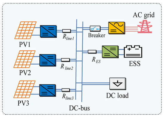
Figure 1.
System configuration of a typical PV-dominated DC microgrid.
To cope with these limitations, a V-P droop governor is designed to enable PV sources to regulate the DC-bus voltage. Figure 2 illustrates a PV generation system, composed of a PV array and a DC/DC buck converter, to demonstrate the overall structure of the proposed control strategy, which is divided into three levels.
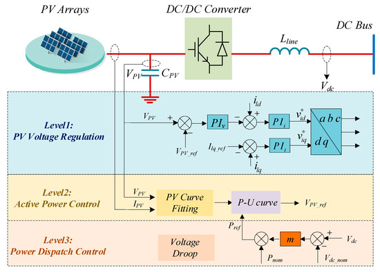
Figure 2.
Structure of the PV source with the proposed control system.
Level 3, the outermost control loop of the proposed control strategy, primarily targets DVR. Different from the traditional V-I droop control scheme, a V-P droop concept is used here to align with the subsequent inner control loops. The input to level 3 is the DC-bus voltage deviation (the difference between its actual value and nominal value), while its output is the PV output power reference . When the DC-bus voltage is at its nominal value, PV sources use the MPPT algorithm and adjust their generation adaptively to provide DVR if the DC-bus deviates from the nominal value. In essence, level 3 determines the PV output power reference according to the DC-bus voltage deviation to provide DVR service, while the inner control loops track the power references.
Level 2 seeks the accurate PV operating voltage corresponding to the power reference provided by level 3, as the PV operating voltage is a common control method for PV sources’ output power. When is lower than the maximum available power point (MAPP), a corresponding to an operating point that is lower than the MAPP needs to be found. When is higher than the MAPP, (the PV operating voltage corresponding to the MAPP) itself should be given out. The inherent nonlinearity in the PV’s P-U curve makes it difficult to solve directly. Generally, there are three categories of solutions: (1) indirect measurement methods relying on irradiation and temperature sensors; (2) searching methods like P and O schemes; and (3) estimation methods. Given the drawbacks of additional measurement sensors and the relatively low convergence rate of P and O methods, this paper enhances conventional estimation methods by introducing a novel characteristic curve. The proposed active power control algorithm’s details are discussed in the following section.
Level 1, the innermost control loop, utilizes a traditional dual-loop control structure to regulate the PV array’s terminal voltage. The outer loop at level 1 controls the PV array voltage and the reactive power, while the inner loop manages the current. Under the control of level 1, when the PV array voltage is equal to supplied by level 2, the PV output power is equal to the required value provided by level 3.
3. Active Power Control Algorithm for Level 2
There exist two complicated issues for flexible power control of PV sources: (1) the P-U characteristic changes if the ambient condition (irradiation and temperature) changes, which means that the PV operating point () varies under different environmental conditions and (2) the same photovoltaic output power has two different operating voltages corresponding to it, except for the MPP. The key point for the PV power control loop can be expressed as follows. For arbitrary power dispatching reference : If is lower than the maximum available power , then find the proper operating voltage (whether lower than the MPP voltage or higher than it but maintaining consistency) to make equal to . If is higher than , then find the MPP voltage. In summary: the main task for PV power control is to find a PV operating voltage that satisfies:
where is the maximum available PV power, G and T are the irradiance and the temperature, respectively, and is the PV’s output power function with PV voltage, irradiation, and temperature being the arguments, respectively.
As stated before, it is hard to obtain as required to solve the for directly. A feasible solution is to use the iterative method based on curve fitting, such as quadratic interpolation. For previous power curtailment algorithms in the literature, the control performance is unsatisfactory because of sensor dependence, computation complexity, or algorithm robustness. Therefore, a characteristic curve fitting-based algorithm is introduced. The basic thought is to use a curve that is similar to the PV’s characteristics to fit the P-U curve and then use an iterative process to obtain the required corresponding to the given . Because of the similarity between the real PV characteristic and the fitting curve, the robustness and the convergence speed of the algorithm can be improved.
3.1. Characteristic PV Curve-Fitting Method
Considering two intersections with the V-axis and the maximum point in the P-U curve of a PV array, a characteristic fitting curve is given as:
where , , and are the fitting coefficients.
Only one point is sampled per iteration. Consider step k in the iterative process, and assume that at least four points on the P-U curve have been sampled. The four sampling points are noted as , , and . The overall strategy in this method is to use the fitted curve, which passes through the four sampling points to imitate the real P-U curve and by continuously iterating to make it locally converged to the target operating point, either the MPP or the power dispatch point. Once at least four sampling points are ready, the following equations are derived from Equation (2):
Next, rewrite Equation (3) in matrix form:
where:
The fitting coefficients can then be solved using or using the least square method if more than four sampling points are kept.
Once the valuables in s are obtained, substitute into Equation (2) and rearrange it to obtain:
which can be regarded as a quadratic equation with being the argument if the active power reference value is given.
Next, we define:
where means that has no intersections with the fitting curve, which indicates that is larger than . Under this circumstance, the PV source should operate in MPPT mode as previously discussed, and the maximum point on the fitted curve is used for the next iteration step. The maximum point can be obtained by solving the zero of the derivative of Equation (2). Thus, the MAPP voltage can be approximated as:
means that is less than the and the PV source now should operate in the APC mode by regulating its output power to . There are two solutions for Equation (5). The uphill segment solution (denoted using UHSS) is derived as:
and the downhill segment solution (denoted by DHSS) is derived as:
Many studies discuss the characteristics of the two solutions for PV voltage regulating. The DHSS shows better control performances in many scenarios. For example, if the power reference is low and far away from , the corresponding UHSS may be too low for the normal operating for a DC/DC Buck converter, while for the DHSS, this will never happen. In addition, the DHSS has better control performances because the UHSS is within the current source region on the PV’s I-V curve, where the output current changes little with the adjustment to the PV voltage. The comparison between the two solutions is beyond the scope of this paper, and we only chose the DHSS as an example. It is worth noting noted that the proposed algorithm applies to both solutions that can be selected.
3.2. Iteration Process
For initialization, at least four different points need to be sampled. The four operating points can be carefully arranged to be evenly distributed on both sides of the MPP, which may speed up the convergence of the algorithm. It is worth mentioning that the proposed algorithm has no strict requirements for the four sampling points for the initialization. Four arbitrary sampling points, for example, four random points within the acceptable operating range, can be used for the algorithm initialization.
For the kth step, using the solutions for Equation (7), Equation (8), or Equation (9), a new can now be calculated, which is fed as the reference to inner loops to track with. For the (k + 1)th step, the corresponding PV voltage and current can be sampled, and then is calculated. If the information on the five points is kept so far, namely (), (), (), (), and () have been obtained, in order to start the next interpolation, one point needs to be removed from the five. In this paper, the most previous point is removed because it represents the information that was sampled at the longest time before as the irradiation and the temperature may change. Then, a new can be calculated according to the same procedure.
As k increases, the iteration continues, and the approximation gradually approaches the desired value. The iteration is considered to be converged if there is only a small difference between and , , , and . The following condition needs to be satisfied:
where is the predefined threshold. Equation (10) indicates that if sampling points are too close, the fitting calculation may result in undesired numerical error. The solution to prevent this is to keep unchanged when Equation (10) is satisfied.
Once the ambient environment conditions change, the algorithm exits the converged state and begins the iteration process towards the new steady state. A flowchart for the proposed APC strategy is shown in Figure 3. The sampling and calculation interval require careful tuning according to the parameters (mainly the control bandwidth) of the inner regulators. Specially, if the bandwidth among different control loops is mismatched, the controller may subject to oscillation or even failure. A not too-large nor too-small guarantees that there is sufficient time for to track with , as well as achieving an acceptable converged rate.
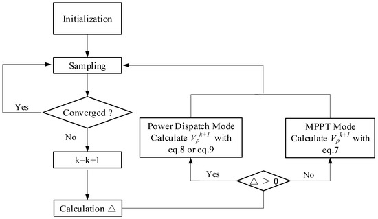
Figure 3.
Flowchart for the proposed APC strategy.
3.3. Comparative Study with the Classical PV Active Power Control Method
This section presents a comparison between the conventional APC method and the proposed one, conducted under identical external and experimental conditions. The quadratic interpolation method proposed in [28] is used as the classical method. Initially, the irradiation was set to 1000 , and it decreased to 100 by a step of 3 s. Then, the irradiation rose to 1200 at 5 s, and subsequently, it recovers to 1000 at 7 s. The PV active power reference value changed from 100 kW to 70 kW at 9 s. The comparative results are shown in Figure 4 and summarized in Table 1.
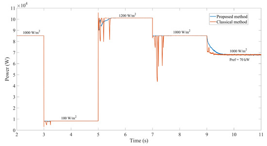
Figure 4.
Dynamics of PV output power under different classical methods and the proposed control method.

Table 1.
Comparison of the test results between the proposed characteristic curve-fitting method and the classical Newton quadratic interpolation method.
The proposed characteristic curve-fitting method significantly reduces overshoots by approximately 80% and 95% when the irradiance transitions from 100 to 1200 and 1200 to 1000 , respectively. The duration is curtailed by about 36%, 78%, and 80% under different test conditions. The results indicate that the proposed method shows better transition performances since significantly fewer disturbances are observed and smoother PV power curves are obtained, especially in the MPPT scenarios. Furthermore, it is worth noting that in our test, for fairness, both methods took the same sample time of 0.02 s, which is the limit for the classical method. If the sample time for the classical method is reduced to 0.01 s, the control performance becomes unacceptable, while the proposed characteristic curve-fitting method can tolerate shorter sampling intervals to further expedite the convergence rate.
4. Droop Control
V-I droop is a widely used technique for voltage regulation and voltage source coordination in DC microgrids. For a traditional V-I type source in DC microgrid, its output current fed into the bus is determined using the deviation in the DC-bus voltage from its nominal value. Specifically, it produces nominal output current (power) when the DC-bus voltage is at its nominal value. If , its output current (power) is below its nominal value , and vice versa.
In this section, the traditional V-I droop strategy is modified to V-P droop control for PV sources to provide primary voltage control. Unlike traditional voltage sources composed of energy storage or DC/AC converter back to the utility grid, (1) there is an upper power limit for the primary source restrictions and (2) the MAPP varies with irradiation and temperature, which requires the droop strategy to be adaptive to various operation conditions.
In response to the aforementioned concerns, a droop function that generates the power references according to the voltage deviation (V-P droop) is used:
where is the PV power reference, (, ) is the nominal operating point, and is the locally sampled DC-bus voltage. The droop coefficient m indicates the change in PV output power per unit voltage deviation, and can be designed as:
According to Equation (11), is calculated without considering the limit of . When reaches the , it takes the value of and thus, the voltage regulation ability is lost. The voltage droop curve is illustrated in Figure 4. The limiting voltage is defined as the voltage at which is equal to :
Obviously, the of the droop characteristic is corresponding to the MAPP and thus is related to irradiation and temperature. Concretely, the PV source generates a maximum available power if is lower than while the source reduces active power generation to reduce the voltage deviation if is higher than . The proposed strategy thus forms the adaption to varying irradiation and temperature. If the irradiation is relatively high, the voltage regulation capability of the PV source is strong, while it is weakened if the solar irradiation is insufficient. For example, it can be seen from Figure 5 that when the irradiation is 800 , the voltage regulation capability is activated only if the DC-bus voltage is higher than 608.5 V (which is the at 800 ), while it is 600 V when the irradiation is 1000 and 592 V when the irradiation is 1200 (with being 85 kW, being 600 V, and m being 2000 ).
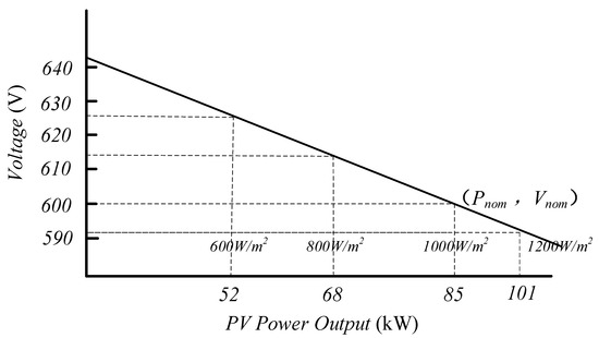
Figure 5.
The proposed V-P droop control curve.
Theoretically, can be selected based on the system requirements. When its value is high, the PV sources cannot provide voltage regulation support at “low” (relatively low) DC-bus voltage. However, when its value is low, the PV sources have stronger voltage regulation capability, but this may sacrifice some benefits at high solar irradiation. Thus, there is a trade-off between economic benefits and voltage regulation capability. In fact, should be selected based on possible disturbances and its original total voltage regulating capability in the system. For example, for a small-scale islanded DC microgrid with high PV penetration, its voltage regulating ability is weak, and more support from PV sources is needed, so should take a low-level value.
5. Case Studies
A comprehensive dynamic model for a DC microgrid, consisting of two PV sources, a V-I droop type voltage source, and two resistance DC loads, was established in Matlab/Simulink for simulation tests. The schematic diagram for the DC microgrid is shown in Figure 6. The specifications of the test system are as follows:
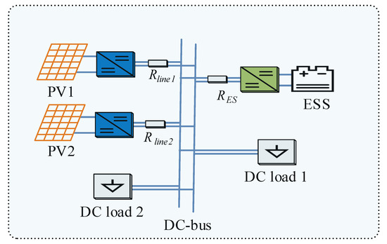
Figure 6.
The DC microgrid system used for simulations.
The ESS maintains the DC-bus voltage of the DC microgrid. The converter of the ESS has a power limit of ±400 kW. A conventional V-I droop concept is implemented, setting the droop coefficient at 0.21 V/A. The nominal voltage and current are set at 600 V and 315 A, respectively. A traditional dual loop control structure is used, with voltage and current regulator gains set to , , respectively.
Two individual PV sources exist within the studied DC microgrid to demonstrate the power sharing coordination under the proposed control strategy. Each PV source has a nominal output power of 85 kW at at 25 °C. If the PV sources use the proposed V-P droop control, the nominal voltage is 600 V with a droop coefficient of 2000 W/V. However, if the PV sources use the MPPT mode, the reference power value is set at 100 kW. The sample interval for the proposed APC algorithm is 0.01 s, with the PV source’s dual loop gains set to , , respectively.
The loads in this simulation study follow a constant resistance model. In scenario 5.1, Load 1# and Load 2# are 3/2 Ω and 3 Ω, respectively, while in scenarios 5.2 and 5.3, Load 1# remains at 3/2 Ω, but Load 2# is altered to 5 Ω.
5.1. Effect of PV Voltage Droop Control
At 15 s, Load 2# (3 Ω), accounting for one-third of the system load, is taken offline. Figure 7 presents a comparative simulation of PV sources operating under traditional MPPT control and those utilizing the proposed voltage droop control. Figure 7a,b illustrates the power outputs of the system storage and the PV sources, respectively, while Figure 7c depicts the dynamics of the DC-bus voltage under both control strategies. Table 2 enumerates the specific values for the test results.
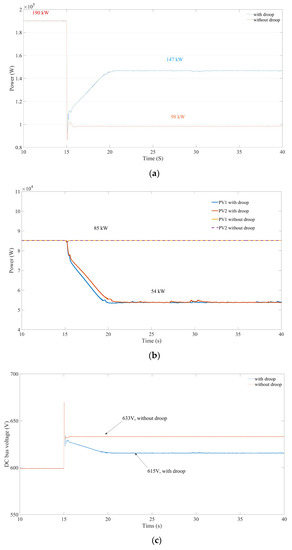
Figure 7.
Response of V-P droop control: (a) storage output power; (b) PV output power; and (c) DC-bus voltage.
Table 2.
Test results under V-P droop control.
Prior to the disconnection of Load 2#, both PV sources, irrespective of the control scheme, operate in the MPPT mode in both scenarios. With an irradiation of , each PV source produces equivalent power output. After 15 s, it can be seen from Figure 7 that with traditional MPPT control scheme, all the power variation in the system (Load 2#) is balanced by the system storage, whose output power decreases from 190 kW to approximately 98 kW. The DC-bus voltage surges significantly, exceeding 633 from an initial value of 600 V.
In contrast, under the proposed V-P droop strategy, the results in Figure 7 indicate that all the PV sources, in conjunction with the system storage, collectively mitigate the power imbalance due to a sudden load change. After 15 s, each PV source gradually reduces its output power by 31 kW, while the system storage only decreases its output power by about 43 kW. Consequently, the DC-bus voltage only ascends to 615 V. Using the proposed DVR strategy results in a power fluctuation of 53.3% in the battery and a voltage deviation decrease of 54.5%, thereby verifying the effectiveness of the proposed strategy in primary voltage regulation.
5.2. Effect of Different Irradiation Levels
In this case, Load 2# (5 Ω), representing 23% of the system load in scenario 5.2, is initially offline and reconnected at 15 s. The simulation results under the four different irradiations (, , , and ) are demonstrated in Figure 8. Figure 8a,b shows the output power of the system storage and the PV sources, respectively. Figure 8c shows the dynamics of the DC-bus voltage. Table 3 details the specific values for the test results.
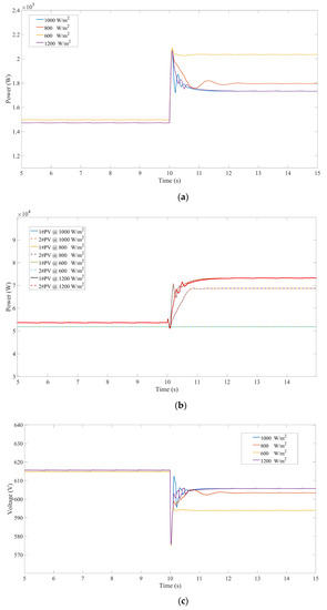
Figure 8.
Simulation results for the system under different irradiations: (a) storage output power; (b) PV output power; and (c) DC-bus voltage.
Table 3.
Test results under different irradiance.
In the initial 10 s, the DC-bus voltages exceed s for irradiations of , and , placing the PV sources into voltage droop mode. However, at 600 , the PV sources operate in the MPPT mode as the DC-bus voltage is beneath the . Upon reconnection of Load 2#, a decrease in DC-bus voltages incites an increase in the PV sources’ output power, based on the V-P droop curve. Figure 8b shows that under low irradiation conditions (here, G = and G = ), the PV sources’ voltage regulation capability is limited, prompting an autonomous and adaptive switch to the MPPT mode. This switch results in a greater proportion of active power being compensated using the storage, leading to a more substantial drop in the DC-bus voltage. Conversely, under relatively high irradiation conditions (here, G = and G = ), the PV sources maintain operation in the voltage regulation mode.
The test results, as detailed in Table 3, confirm that PV sources under higher solar irradiation have a stronger capacity for voltage regulation, with observed voltage drops of 10 V, 10 V, 12 V, and 21 V under the respective irradiance of , , , and . If the original voltage regulation capability of the system is not sufficient, it is necessary to set a lower value, thereby enabling the PV sources to exert a stronger voltage regulation capacity.
5.3. Responses to Step-Changed Conditions
This case is designed to assess system responses under drastic step-changed conditions, encompassing both the step-changed irradiance shift from 1000 and 100 and the step-changed online/offline load transition of 240 kW, accounting for nearly 80% of the total system load. Figure 9 illustrates the DC-bus voltage under these significant step-changed conditions.
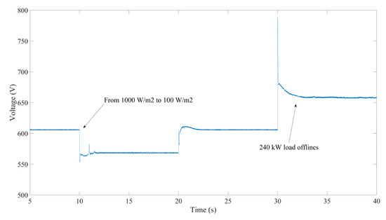
Figure 9.
DC-bus voltage under the step-changed conditions.
As depicted in Figure 9, the initial irradiance is set at 1000 , maintaining the DC-bus voltage at 606 V. At 10 s, the irradiance abruptly decreases to 100 to simulate the potential extreme real-world scenarios. Following minor oscillations (attributed to fluctuations in PV generation), the DC-bus voltage stabilizes to a steady state within about 2 s. The irradiance restores to 1000 at 20 s, while about 80% of the system’s total load is cutoff at 30 s. A considerable overshoot in the DC-bus voltage is observed, amounting to roughly 19.3% of the nominal voltage, but it rapidly stabilizes at 658 V. The precise values of the test results are detailed in Table 4. The maximum voltage overshoot is around 19.3%, and the longest response time is 3 s, signifying the proposed voltage regulation strategy’s robustness and adaptability to varied working conditions.
Table 4.
Test results under step-changed conditions.
5.4. Real World Project Analysis
The proposed DC-bus voltage regulation strategy was practically implemented in a commercial DC microgrid project in Shaoxing, Zhejiang Province, China, specifically within the “shijihuatong” industrial park in Shangyu District. Figure 10 presents photographs of the microgrid’s critical components, while a schematic diagram is depicted in Figure 11. Within this DC microgrid, photovoltaic (PV) arrays on factory roofs serve as the primary renewable sources, and the inductors of injection molding machines constitute the major DC loads. These machines are driven with DC/AC converters, having eliminated the former AC/DC conversion stage for enhanced efficiency. Other DC loads include light-emitting diode (LED) lights and charging stations for electric vehicles. By integrating the DC loads and sources within a single DC bus, then the overall system efficiency improves. Unlike many low-voltage DC microgrids, this system’s DC-bus voltage is set at 560 V for optimal connectivity with the DC/AC drivers of the injection molding machines. Key component parameters of the DC microgrid are detailed in Table 5.
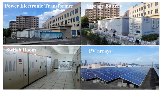
Figure 10.
Photos of the “Shijihuatong” DC microgrid.
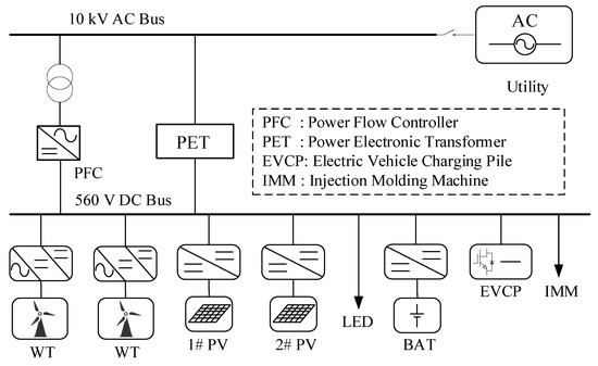
Figure 11.
Schematic diagram showing the DC microgrid.
Table 5.
Components of the DC microgrid.
The droop coefficient of the BAT is 0.21 A/V, and the nominal current is 315 A. The V-P droop coefficient of the PV source is 2 kW/V. Comparative tests between the conventional MPPT control and the proposed DVR strategy were performed to validate the improvement and effectiveness of the proposed strategy. In both experiments, the system’s initial total load stands at approximately 316 kW, with the DC-bus voltage maintained at its nominal value, and each PV source output at around 220 kW. The tests simulate a sudden step-change in load by disconnecting LED lights and EVCPs, amounting to roughly 100 kW DC load. Figure 12 and Figure 13 depict system responses under both control strategies, and the specific values in Table 6 show that involving PV sources in DVR services reduces DC-bus voltage deviation by approximately 25%.
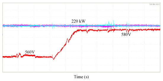
Figure 12.
System responses under MPPT control. The blue line shows the output power from the 1# PV source, the pink line shows the output power from the 2# PV source, and the red line shows the DC-bus voltage.
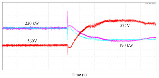
Figure 13.
System responses under the proposed DVR strategy. The blue line shows the output power from 1# PV source, the pink line shows the output power from 2# PV source, and the red line shows the DC-bus voltage.
Table 6.
Test results for the real DC microgrid.
It should be noted that the algorithm’s control effect is contingent on the parameter settings. Although a large V-P droop coefficient for the PV sources may enhance voltage regulation, it could simultaneously increase PV generation loss. This necessitates a balance between DVR capabilities, PV generation benefits, and parameter settings, taking into account potential disturbances, total regulation capacity, and economic benefits, among other factors.
6. Conclusions
This paper presents a novel voltage regulation strategy for PV sources in DC microgrids. Firstly, a characteristic curve-fitting method is proposed to regulate the PV output power flexibly and accurately. Using a PV characteristic curve that closely resembles a real PV’s P-U curve, the control performance and robustness are enhanced. The comparative study results demonstrate that voltage overshoot can be mitigated by up to 95%, and the response speed can be improved by up to 80%. Based on the proposed active power control method, a novel V-P type droop control is designed, enabling PV sources to provide primary voltage regulation services. Using this control strategy, PV sources could adaptively participate in the system voltage regulation or maintain in the MPPT mode, according to the voltage levels and the irradiance. When irradiance is sufficient and the DC-bus voltage surpasses its nominal value, the PV source will backoff some of its maximum available power in relation to the voltage deviations. The voltage regulation capability weakens with decreasing irradiance. A real-world project analysis validates that this strategy can reduce the voltage deviation by about 25% during a 30% load shedding, which can be further improved using parameter setting.
The proposed control strategy is straightforward to implement as it does not require additional sensors, communication networks, or complex calculations. This significantly minimizes installation and maintenance costs, thereby enhancing the strategy’s practical applicability. However, it is crucial to consider the setting of the nominal point for PV sources for the equilibrium between solar generation benefits and voltage regulation capability. Hence, a trade-off exists between economic benefits and voltage regulation capability. Taking these considerations into account, the proposed strategy could be further refined in terms of optimal nominal point selection to amplify the penetration and exploitation of PV sources, applicable to both distributed sources and large PV plants.
Author Contributions
Conceptualization, J.L. and W.W.; Methodology, H.C. and Y.W.; Software, Y.W.; Validation, H.C. and Y.W.; Formal analysis, Y.W.; Investigation, H.C. and Y.W.; Writing–original draft, H.C.; Writing–review & editing, H.C.; Supervision, J.L. and W.W.; Project administration, J.L. and W.W.; Funding acquisition, W.W. All authors have read and agreed to the published version of the manuscript.
Funding
This research was funded by “Pioneer” and “Leading Goose” R & D Program of Zhejiang, grant number 2023C01126.
Data Availability Statement
The data presented in this study are available on request from the corresponding author.
Conflicts of Interest
The authors declare no conflict of interest.
References
- Xia, Y.; Lv, Z.; Wei, W.; He, H. Large-Signal Stability Analysis and Control for Small-Scale AC Microgrids with Single Storage. IEEE J. Emerg. Sel. Top. Power Electron. 2021, 10, 4809–4820. [Google Scholar] [CrossRef]
- Xia, Y.; Peng, Y.; Yang, P.; Li, Y.; Wei, W. Different Influence of Grid Impedance on Low- and High-Frequency Stability of PV Generators. IEEE Trans. Ind. Electron. 2019, 66, 8498–8508. [Google Scholar] [CrossRef]
- Xin, H.; Liu, Y.; Wang, Z.; Gan, D.; Yang, T. A New Frequency Regulation Strategy for Photovoltaic Systems Without Energy Storage. IEEE Trans. Sustain. Energy 2013, 4, 985–993. [Google Scholar] [CrossRef]
- Yang, P.; Yu, M.; Wu, Q.; Hatziargyriou, N.; Xia, Y.; Wei, W. Decentralized Bidirectional Voltage Supporting Control for Multi-Mode Hybrid AC/DC Microgrid. IEEE Trans. Smart Grid 2019, 11, 2615–2626. [Google Scholar] [CrossRef]
- Yang, P.; Yu, M.; Wu, Q.; Wang, P.; Xia, Y.; Wei, W. Decentralized Economic Operation Control for Hybrid AC/DC Microgrid. IEEE Trans. Sustain. Energy 2020, 11, 1898–1910. [Google Scholar] [CrossRef]
- Xia, Y.; Long, T. Chopperless Fault Ride-Through Control for DC Microgrids. IEEE Trans. Smart Grid 2021, 12, 965–976. [Google Scholar] [CrossRef]
- Wang, X.; Peng, Y.; Weng, C.; Xia, Y.; Wei, W.; Yu, M. Decentralized and Per-Unit Primary Control Framework for DC Distribution Networks With Multiple Voltage Levels. IEEE Trans. Smart Grid 2020, 11, 3993–4004. [Google Scholar] [CrossRef]
- Xia, Y.; Wei, W.; Long, T.; Blaabjerg, F.; Wang, P. New Analysis Framework for Transient Stability Evaluation of DC Microgrids. IEEE Trans. Smart Grid 2020, 11, 2794–2804. [Google Scholar] [CrossRef]
- Rajan, R.; Fernandez, F.M.; Yang, Y. Primary frequency control techniques for large-scale PV-integrated power systems: A review. Renew. Sustain. Energy Rev. 2021, 144, 110998. [Google Scholar] [CrossRef]
- Varma, R.K.; Siavashi, E.; Mohan, S.; McMichael-Dennis, J. Grid Support Benefits of Solar PV Systems as STATCOM (PV-STATCOM) through Converter Control: Grid Integration Challenges of Solar PV Power Systems. IEEE Electrif. Mag. 2021, 9, 50–61. [Google Scholar] [CrossRef]
- Omran, W.A.; Kazerani, M.; Salama, M.M.A. Investigation of Methods for Reduction of Power Fluctuations Generated from Large Grid-Connected Photovoltaic Systems. IEEE Trans. Energy Convers. 2011, 26, 318–327. [Google Scholar] [CrossRef]
- Sangwongwanich, A.; Yang, Y.; Blaabjerg, F. High-Performance Constant Power Generation in Grid-Connected PV Systems. IEEE Trans. Power Electron. 2016, 31, 1822–1825. [Google Scholar] [CrossRef]
- Zhong, C.; Zhou, Y.; Yan, G. A Novel Frequency Regulation Strategy for a PV System Based on the Curtailment Power-Current Curve Tracking Algorithm. IEEE Access 2020, 8, 77701–77715. [Google Scholar] [CrossRef]
- Zhong, C.; Zhou, Y.; Zhang, X.; Yan, G. Flexible power-point-tracking-based frequency regulation strategy for PV system. IET Renew. Power Gener. 2020, 14, 1797–1807. [Google Scholar] [CrossRef]
- Zhu, Y.; Wen, H.; Bu, Q.; Wang, X.; Hu, Y.; Chen, G. An Improved Photovoltaic Power Reserve Control With Rapid Real-Time Available Power Estimation and Drift Avoidance. IEEE Trans. Ind. Electron. 2022, 70, 11287–11298. [Google Scholar] [CrossRef]
- Wang, Z.; Yi, H.; Zhuo, F.; Lv, N.; Ma, Z.; Wang, F.; Zhou, W.; Liang, J.; Fan, H. Active Power Control of Voltage-Controlled Photovoltaic Inverter in Supporting Islanded Microgrid Without Other Energy Sources. IEEE J. Emerg. Sel. Top. Power Electron. 2021, 10, 424–435. [Google Scholar] [CrossRef]
- Wandhare, R.G.; Agarwal, V. Advance Control Scheme and Operating Modes for Large Capacity Centralised PV-Grid Systems to Overcome Penetration Issues. In Proceedings of the 2011 37th IEEE Photovoltaic Specialists Conference, Seattle, WA, USA, 19–24 June 2011; pp. 002466–002471. [Google Scholar]
- Cai, H.; Xiang, J.; Wei, W.; Chen, M.Z.Q. Droop Control for PV Sources in DC Microgrids. IEEE Trans. Power Electron. 2017, 33, 7708–7720. [Google Scholar] [CrossRef]
- Cai, H.; Xiang, J.; Wei, W. Decentralized Coordination Control of Multiple Photovoltaic Sources for DC Bus Voltage Regulating and Power Sharing. IEEE Trans. Ind. Electron. 2018, 65, 5601–5610. [Google Scholar] [CrossRef]
- Chang, Y.-C.; Kuo, C.-L.; Sun, K.-H.; Li, T.-C. Development and Operational Control of Two-String Maximum Power Point Trackers in DC Distribution Systems. IEEE Trans. Power Electron. 2013, 28, 1852–1861. [Google Scholar] [CrossRef]
- Shadmand, M.B.; Balog, R.S.; Abu-Rub, H. Model Predictive Control of PV Sources in a Smart DC Distribution System: Maximum Power Point Tracking and Droop Control. IEEE Trans. Energy Convers. 2014, 29, 913–921. [Google Scholar] [CrossRef]
- Yang, P.; Peng, Y.; Xia, Y.; Wei, W.; Yu, M.; Feng, Q. A unified bus voltage regulation and MPPT control for multiple PV sources based on modified MPC in the DC microgrid. Front. Energy Res. 2022, 10, 1010425. [Google Scholar] [CrossRef]
- Elrayyah, A.; Sozer, Y.; Elbuluk, M.E. Modeling and Control Design of Microgrid-Connected PV-Based Sources. IEEE J. Emerg. Sel. Top. Power Electron. 2014, 2, 907–919. [Google Scholar] [CrossRef]
- Hoke, A.F.; Shirazi, M.; Chakraborty, S.; Muljadi, E.; Maksimovic, D. Rapid Active Power Control of Photovoltaic Systems for Grid Frequency Support. IEEE J. Emerg. Sel. Top. Power Electron. 2017, 5, 1154–1163. [Google Scholar] [CrossRef]
- Liao, S.; Xu, J.; Sun, Y.; Bao, Y.; Tang, B. Wide-area measurement system-based online calculation method of PV systems de-loaded margin for frequency regulation in isolated power systems. IET Renew. Power Gener. 2017, 12, 335–341. [Google Scholar] [CrossRef]
- Subha, R.; Himavathi, S. Active power control of a photovoltaic system without energy storage using neural network-based estimator and modified P&O algorithm. IET Gener. Transm. Distrib. 2018, 12, 927–934. [Google Scholar] [CrossRef]
- Chen, X.; Xu, X.; Wang, J.; Fang, L.; Du, Y.; Lim, E.G.; Ma, J. Robust Proactive Power Smoothing Control of PV Systems Based on Deep Reinforcement Learning. IEEE Trans. Sustain. Energy 2023, 14, 1585–1598. [Google Scholar] [CrossRef]
- Liu, Y.; Xin, H.; Wang, Z.; Yang, T. Power control strategy for photovoltaic system based on the Newton quadratic interpolation. IET Renew. Power Gener. 2014, 8, 611–620. [Google Scholar] [CrossRef]
- Batzelis, E.I.; Kampitsis, G.E.; Papathanassiou, S.A. Power Reserves Control for PV Systems with Real-Time MPP Estimation via Curve Fitting. IEEE Trans. Sustain. Energy 2017, 8, 1269–1280. [Google Scholar] [CrossRef]


Disclaimer/Publisher’s Note: The statements, opinions and data contained in all publications are solely those of the individual author(s) and contributor(s) and not of MDPI and/or the editor(s). MDPI and/or the editor(s) disclaim responsibility for any injury to people or property resulting from any ideas, methods, instructions or products referred to in the content. |
© 2023 by the authors. Licensee MDPI, Basel, Switzerland. This article is an open access article distributed under the terms and conditions of the Creative Commons Attribution (CC BY) license (https://creativecommons.org/licenses/by/4.0/).