Article

Exploring the Impact of Vehicle Lightweighting in Terms of Energy Consumption: Analysis and Simulation

Department of Mechanical and Industrial Engineering, University of Brescia, I-25123 Brescia, Italy
*
Author to whom correspondence should be addressed.
Energies 2023, 16(13), 5157; https://doi.org/10.3390/en16135157
Submission received: 25 May 2023 / Revised: 19 June 2023 / Accepted: 29 June 2023 / Published: 4 July 2023
(This article belongs to the Section E: Electric Vehicles)

Abstract

:
Nowadays, the topic of reducing vehicles’ energy consumption is very important. In particular, for electric vehicles, the reduction of energy consumption is necessary to remedy the most critical problems associated with this type of vehicle: the problem of the limited range of the electric traction, also associated with the long recharging times of the battery packs. To reduce use-phase impacts and energy consumptions of vehicles, it is useful to reduce the vehicle mass (lightweighting). The aim of this work is to analyze the parameters of a vehicle which influence the results of lightweighting, in order to provide guidelines for the creation of a vehicle model suitable for studying the effects of lightweighting. This study was carried out through two borderline case models, a compact car and an N1 vehicle, and simulating these through a consolidated vehicle simulation tool useful for consumption estimations. This study shows that the parameters that most influence the outcome of lightweighting are the rolling resistance, the battery pack characteristics, the aerodynamic coefficients, and the transmission efficiency, while the inertia contributions can be considered negligible. An analysis was also carried out with the variation of the driving cycle considered.

1. Introduction

Nowadays, the topic of reducing consumption is very important, both for internal combustion vehicles and for electric vehicles. In fact, fuel saving for internal combustion vehicles is very important, in particular due to the issue of emissions and the related stringent laws [1,2]. Meanwhile, for electric vehicles, the reduction of energy consumption is necessary to remedy the most critical problems associated with this type of vehicle: the problem of the limited range of the electric traction, also associated with the long recharging times of the battery packs [3].
The fuel or energy consumption of vehicles is due to two components [4]: the displacement of the mass of the vehicle and the contribution given by various losses (for example, aerodynamic drag, accessories, engine, and powertrain friction) [5,6,7,8,9].
To reduce the use-phase impacts and fuel or energy consumptions of vehicles [4,10] the following are useful:
  • To have improved powertrains and engine efficiency (high-efficiency internal combustion, electric, and hybrid) [11,12,13,14,15];
  • To use more environmentally sustainable sources of energy such as electric or hybrid traction, alternative fossil fuels, and biofuels [16];
  • To improve the aerodynamics of vehicles [17];
  • To reduce the vehicle mass (lightweighting) [5,17,18,19,20];
  • To implement speed control to reduce the fuel or energy consumption and therefore the impacts during vehicle use [10];
  • To plan more sustainable routes and introduce more connected vehicles [10,21];
  • To educate users to have more sustainable driving behaviors [22].
However, it is good to keep in mind that any intervention must be compatible with other needs, in particular with safety [10,23].
In this paper, we will focus on the lightweighting of electric vehicles as a method for reducing consumption. The latter issue is very important, considering the low traction range and long battery recharge times associated with fully electric vehicles. Deepening the topic of electric vehicles is very important. In fact, the European Parliament voted, on Wednesday, 8 June 2022, to stop sales of new ICE cars and vans in EU starting from 2035 (ordinary legislative procedure 2021/0197(COD) [24]).
In particular, lightweighting can be achieved in several ways:
  • The most common method is material substitution as well as design and construction changes [4,12,18,25,26,27] (considering also the role of plastics in lightweighting [28]);
  • Adopting solutions with alternative powertrains, for example, a fuel cell/battery pack hybrid electric system, adding the complexity and weight given by the additional components of the system, can allow the total weight of the powertrain to be reduced thanks to the downsizing of the battery pack;
  • Implementing suitable regenerative braking logics and range management [29];
  • Improving energy dense battery chemistries [29] and, in general, battery weight optimization;
  • Improving the battery efficiency, for example, through different and more efficient systems of battery cooling, in such a way as to be able to reduce battery size for the same vehicle range;
  • Adopting other, more weight-efficient battery forms and shapes, such as blade batteries and structural battery packs;
  • Secondary mass saving and resizes.
Paper [4] describes 10 lightweighting principles, focused on environmental sustainability, but also considering economic and social aspects. Principle 9 of [4] is about the evaluation of additional benefits resulting from component and vehicle lightweighting, such as secondary mass saving and resizes and alternative powertrains [27,30,31]. In fact, the mass of some vehicle components depends on the mass of others [30,31]. The total mass reduction in these components is known as secondary mass savings. Mass reduction alters the vehicle’s performance, so the powertrains can be resized to re-establish the original vehicle performance. This results in improved fuel efficiency [6,32,33,34]. Increased fuel efficiency enables an increase in vehicle range, with the same capacity of the tank or the same capacity of the battery pack.
Paper [10] investigates the lightweighting strategy of material substitution and mass reduction, but without ignoring shape optimization, the controls, and the production processes. In particular, the study discriminates the environmental benefits according to the size of the vehicle and its power supply (i.e., gasoline, hybrid, and electric). Paper [10] distinguishes vehicles according to their size but does not specify whether it is the mass of the vehicle that causes the different results of lightweighting or whether some other parameter of the vehicle which varies according to the vehicle class. In this paper, therefore, we ask ourselves why, by reducing the mass of two vehicles of different classes by the same amount, the variation in consumption is different. In particular, we want to understand if this aspect is due to the non-linearity of the vehicle consumption–weight curve or if there are other vehicle parameters that come into play. The answer lies also in this second aspect. In this paper, the parameters of the vehicle which lead to a different behavior following lightweighting will therefore be investigated.
Furthermore, the study [10] covers the lightweighting aspects associated with different components of a vehicle and adds up all its beneficial contributions:
  • Engine compartment, where the improvement concerns the aesthetic cover of the engine, replacing the traditional one in fiberglass with one made with bio-based fiber materials [35];
  • Frame, in particular the substitution of its main constituting parts;
  • Bodywork, considering the material substitution, the production processes, and modifying the geometries;
  • Wheels, considering different type of tires, brakes, and suspension arms;
  • Passenger compartment;
  • Electronics and electrical system, considering the introduction of a speed control system [36] (reduction of the maximum speed of the vehicle on motorways from 130 to 120 km/h and reduction of consumption by 6% in a medium-sized gasoline car), and the replacement of traditional copper electrical cables with those in copper-tin (Cu-Sn) of reduced diameter and mass [37]; although, it should be noted that Cu-Sn can only be used in low current or signal applications (e.g., measurement signals of the voltages of the single cells of the battery pack) and not in the power connection cables due to a resistance increase [38].
However, this last aspect does not concern lightweighting and also makes changes to the vehicle’s maximum performance.
Ref. [10] says that the greatest advantage obtained thanks to lightweighting is found in internal combustion vehicles, while there is a lesser advantage on electric vehicles. Meanwhile, in terms of size, it is small cars that benefit most from weight reduction [10]. Considering that due to the recent stringent laws, thermal combustion vehicles are destined to disappear, it is important to analyze, in more detail, the benefits that various lightweighting techniques can bring to electric vehicles. In this paper, we will focus precisely on the latter.
Paper [39] considers different alloy and technologies of components manufacturing with the aim of lightweighting, considering the transition from an internal combustion engine to electric vehicles. Ref. [39] says that the goal of a lightweight design is to build structures with minimal use of materials and an optimized use of material strength.
In the literature, many papers express the results of lightweighting using the Fuel Reduction Value (FRV), expressed in L/(100 km ∙ 100 kg), where L represents the liter of gasoline or diesel, saved to travel 100 km, following a vehicle mass reduction of 100 kg. Typically, in the literature, FRV indices calculated through experimental tests in previous works are used [34].
Paper [34] estimates fuel consumption during use-phase, associated with a vehicle lightweighting process, calculating the FRV using a method created ad hoc, based on the U.S. Environmental Protection Agency (EPA) databases. Paper [6] presents a work similar to what is reported in [34] but is specific to electric vehicles, thus considering the FRV expressed in equivalent liters per 100 km and per 100 kg of lightweighting, since the traction of electric vehicles is guaranteed by the electric energy of the battery pack and not from the liters of fuel used to feed the internal combustion engine. Both articles ([6,34]) evaluate the aspect of lightweighting from an LCA (Life Cycle Assessment) perspective [40,41,42].
Papers [43,44] also evaluate the effects of lightweighting in the automotive sector from an LCA perspective. Ref. [43] calculates the FRV coefficient for a wide range of gasoline turbocharged vehicle case studies and [44] for diesel turbocharged vehicles. In particular, both papers show how the FRV varies according to the vehicle class considered, distinguishing vehicles in A/B, C, and D classes, but without showing which vehicle parameters actually lead to this variation. Instead, the research and analysis of the vehicle parameters that influence the results of lightweighting represent the work proposed in this paper.
Other scientific articles that deal with the lightweighting topic from an LCA perspective are [5,45]. Ref. [5] calculates the FRV coefficient by also considering the secondary lightweight effects. Ref. [45] evaluates the vehicle use stage for both internal combustion engine vehicles (ICEVs) and electric vehicles (EVs): in particular, the classical FRV coefficient is used for ICEVs, while the ERV index is used for EVs. In fact, the ERV coefficient is more suitable when electric vehicles are considered, being expressed in kWh/(100 km ∙ 100 kg). Indeed, it is possible to have a more immediate representation, considering the energy consumption savings (expressed in kWh/100 km) associated with 100 kg of mass reduction, without having to go through the equivalent liters of fuel.
Finally, paper [46] focuses on electric vehicles to evaluate the results of lightweighting, proposing a methodology for calculating the ERV index. In addition, in the work proposed in our paper, we focus on electric vehicles and, therefore, it was decided to evaluate the effects of lightweighting based on the ERV coefficient instead of the FRV, considering the ERV index, expressed in kWh/(100 km ∙ 100 kg), to be more suitable and more comfortable, not having to refer to the equivalent liters of petrol or diesel which are not directly involved in electric traction.
As seen above, the topic of vehicle lightweighting is treated in the literature in various forms, often referring to or calculating the FRV index (or ERV in the case of electric vehicles). These indices differ according to the class of the vehicle being studied, but there is no study in the literature concerning which vehicle parameters lead to this variability. This last aspect is precisely the subject matter of the study presented in this paper, which, being focused on full electric vehicles, deals with the lightweighting topic by referring to the ERV coefficient. The ultimate objective of this work is therefore to evaluate which are the parameters of the vehicle to be estimated more accurately for the realization of a model useful for evaluating the effects of lightweighting.
This paper is organized as follows:
  • Section 2 shows the methodology adopted, in particular the reference vehicles of this study, the driving cycle used for the energy consumption estimation, the simulation tool adopted, the vehicle parameters that are the object of investigation, and a brief explanation of the simulations carried out;
  • Section 3 presents the results of the study and the considerations that derive from it;
  • In Section 4, the results obtained in Section 3 are discussed and reorganized, and some future works are presented;
  • In Section 5, some concluding remarks are reported, and the most relevant information in Section 4 is summarized.
In particular, it has been found that for a correct calculation of the ERV index, it is important, first, to establish the correct definition of the rolling resistance coefficient, followed by the aerodynamics, and then the battery pack parameters and the transmission efficiency. On the other hand, the inertia contribution can be considered negligible.

2. Materials and Methods

The objective of this research is to evaluate which are the parameters of the vehicle (and its model) that influence the results of lightweighting, all with reference to vehicle categories M and N1 [47]. For the analysis, various simulations were carried out with the model described in [48] (with the integrations described in [49,50]), for the estimation of energy consumption, on standard driving cycles, as the mass of the vehicle varies.

2.1. Reference Vehicles

Two opposite cases were considered, a utility car (compact car, segment B, category M) and a light commercial vehicle (category N1).
In particular, the N1 category vehicle is the vehicle adopted in [48] for the validation of the model with a low performance vehicle, but with a total vehicle transmission ratio equal to 6.22. Despite the modification of the transmission ratio, the vehicle in question fails to follow the standard driving cycles presented later for high vehicle weights (around 3500 kg). To exclude the variability of the results given by the limitations imposed by the maximum performance of the electric motor and the battery pack, appropriate measures have been adopted in order to avoid the occurrence of these limitations: an increase of the maximum motor torque and of the maximum current that can be supplied by the battery pack.
The compact vehicle of VI-CarRealTime (VI-Grade), the “CompactCar”, was considered as a B-segment vehicle. VI-Grade vehicle models are validated. In fact, as the VI-CarRealTime documentation explains, all VI system data could either come from experimental tests performed in a lab or from a virtual test performed within Adams Car. However, this VI-Grade vehicle is equipped with an internal combustion engine; therefore, only the characteristics of the vehicle layout have been maintained (wheels, aerodynamics, etc.), while the driveline has been replaced with that of a compact electric car widely marketed in Italy and Europe, the “Fiat 500e Hatchback 42 kWh” [51,52], which has an electric motors power of 87 kW, a single transmission total reduction ratio of 9.6, and a battery pack of 42 kWh.
For more details on vehicle (compact car and N1 vehicle) parameters, see Table 1.
Initially, both vehicles (compact car and N1 vehicle) were considered equipped with a classic benchmark regenerative braking logic, with a trend as a function of time typically found in the literature [48,49]. In particular, the maximum possible regenerative torque is equal to 50 Nm for both vehicles, and the regenerative recovery begins when the accelerator pedal is released or, in any case, when the driver presses the brake pedal (and the accelerator pedal is not pressed), with a linear increment equal to 22.5 Nm/s. The simulations with vehicles equipped with a regenerative braking logic led to considerations (which we will see later) which meant that the analysis of the results of lightweighting was then carried out on the same vehicles, but without regenerative recovery under braking.

2.2. Driving Cycle

The effects of lightweighting on the two vehicles were evaluated on the following standard driving cycles:
  • WLTC (Worldwide Harmonized Light-Duty Vehicles Test Cycle), class 3b, driving cycle described in the WLTP (Worldwide Harmonized Light-Duty Vehicles Test Procedure) procedure [53];
  • SFTP-US06, described in the “EPA Supplemental Federal Test Procedure” (SFTP) [54];
  • FTP75 (EPA Federal Test Procedure) [55];
  • HWFET (EPA Highway Fuel Economy Cycle);
  • Japanese JC08 Emission Test Cycle [56];
  • Artemis, Urban, Rural Road, and Motorway (130) Cycle [57].

2.3. Simulation Tool

For the simulation, the TEST (Target-speed EV Simulation Tool) model [48] was used, a vehicle longitudinal dynamics simulation tool that allows the simulation of both the mechanical and the electrical parts of full electric or hybrid electric vehicles.
The model is described in [48] (for more details, see also [58,59]), with the integration shown in [49,50,60].
However, further improvements have been made to the tool, aimed at facilitating the setting up of the simulations (and the vehicle model parameters) and their iterations, as the mass of the vehicle varies:
  • The possibility to save and use vehicle databases;
  • The automation of iterations according to three logics.
First, thanks to an additional panel of the graphical user interface, using an on/off switch, it is possible to choose whether to use a pre-set database or to manually enter the parameters of the vehicle being simulated. Through a list-by-list procedure, it is possible to choose one of the possible databases. Meanwhile, through a button, it is possible to create a new database or modify existing databases, regarding the constant parameters. Furthermore, the panel also has several other buttons for modifying the vectorial parameters of the vehicle model related to the chosen database. Instead, through another button, it is possible to charge the constant vehicle model parameters related to the database chosen and use them for the TEST model simulations.
The TEST model has also been integrated with the addition of the possibility of simulation iterations, through the following three logics:
  • Defining the number of simulations to be performed, where the initial SOC of the next simulation is equal to the final SOC of the previous simulation;
  • By defining a minimum SOC, the initial SOC of the next simulation is equal to the final SOC of the previous simulation; the iterations continue until the final SOC falls below the minimum SOC set;
  • Iterations by varying the weight of the vehicle, in particular, an iteration is performed with the empty weight of the vehicle, defined in the model variables. A settable number of iterations are also performed, with a constant weight increase to be defined for each simulation with respect to the previous one. The same procedure is conducted for weight reduction, starting from the unladen weight of the vehicle set as the default value.
The main features of this tool are the short computation times and the execution of closed-loop simulations that are more efficient than other tools reported in the literature [58]. This instrument is reliable, robust, and numerically stable. It is also intuitive and easy to use for people without specific training. Finally, the graphical user interface is simple and straightforward.
However, due to various approximations adopted (for example, the absence of the Pacejka for the tires, the approximation of the condition of perfect rolling of the tires without slip, and the fact of not considering the variation of the wheel radius during the simulations), the TEST model results are less accurate than other simulation tools, such as the one presented in [58], widely used by our research group. This is not a problem for the project proposed here. Since the TEST model simulates low performance road vehicles very well, it has limitations only for vehicles with very high performance (e.g., the hypercar considered in the validation phase of the model [48]), for which a calibration of the model is required.

2.4. Parameters of the Vehicle (and of Its Model) Which Can Affect the Lightweighting Results

Analyzing the parameters and the structure of the TEST model [48], the following parameters were identified, which can influence the variability of the results of lightweighting according to the type of vehicle and its characteristics.
  • Driving cycle considered: different phases of acceleration and deceleration, different intensities of the latter, different powers involved, and variation of the possibility of regenerative recovery.
  • Rolling resistance coefficient: in fact, the latter appears in the mathematical formula of the rolling resistance together with the mass of the vehicle.
  • Coefficients of aerodynamic resistance: these realize the aerodynamic resistance force acting on the vehicle. In the mathematical formula of the latter, the mass does not appear, but, for the same driving cycle, this force modifies the proportion between phases in which the electric motor is delivering torque (both in acceleration and deceleration) and those (in deceleration) in which the electric motor does not deliver torque or, alternatively, which acts as a generator recharging the battery pack. In fact, during deceleration, it is possible to have a lower deceleration than that which would occur in the event of an electric motor not delivering torque. Deceleration therefore is due solely to resisting forces, inertia, etc. Therefore, in the event of lower deceleration, the electric motor will still have to deliver torque. The result will therefore not be actual braking but a partial release of the accelerator pedal. Furthermore, aerodynamic resistance is a function of speed, and at different speeds of the driving cycle, it is possible to have different acceleration values, with which the contribution of the vehicle mass is correlated, due to the resulting inertia. The acceleration contribution can therefore have a different influence at different points in the driving cycle, as can the mass contribution but not in a corresponding way.
  • Other parameters that may be useful to investigate are listed below:
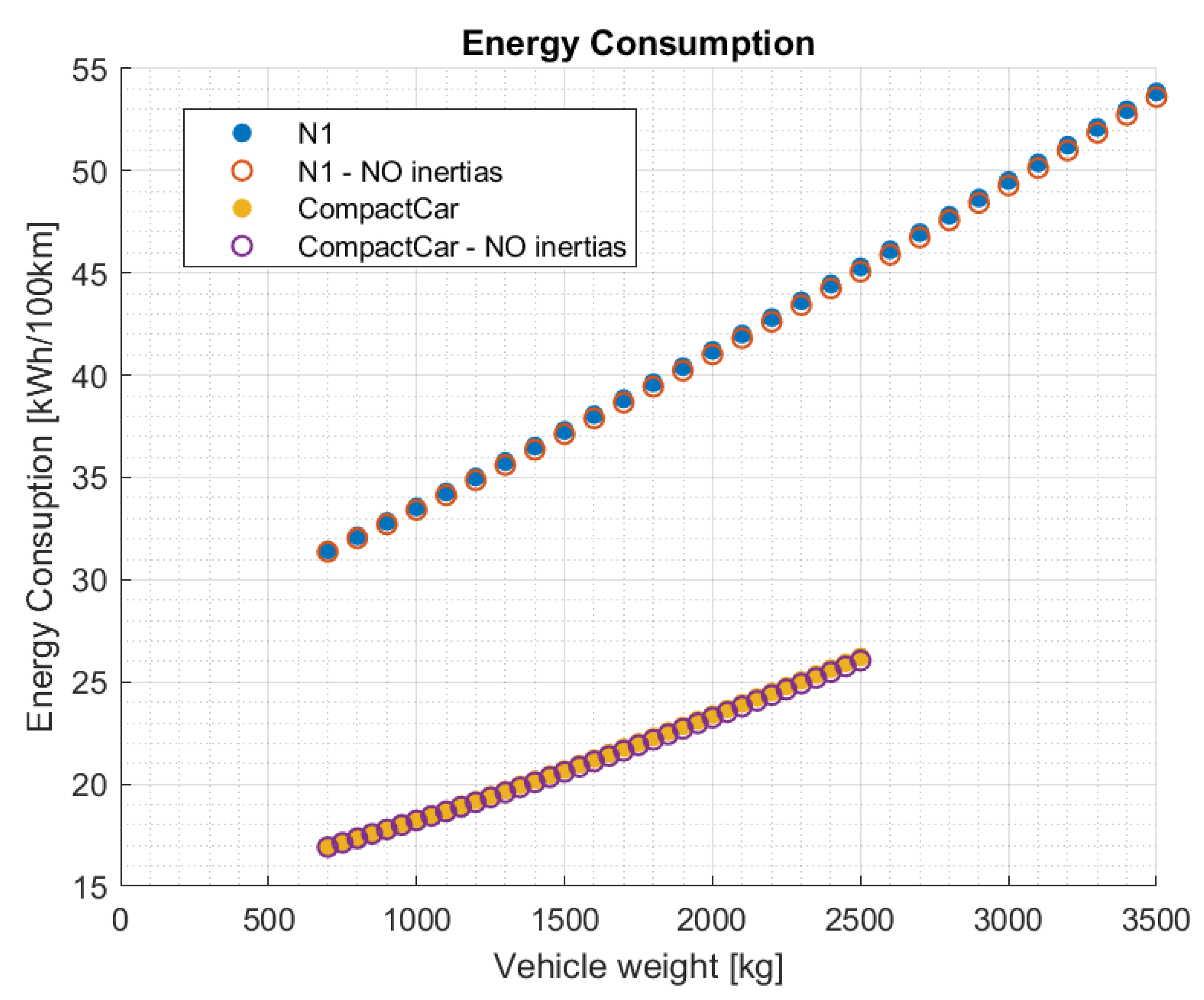
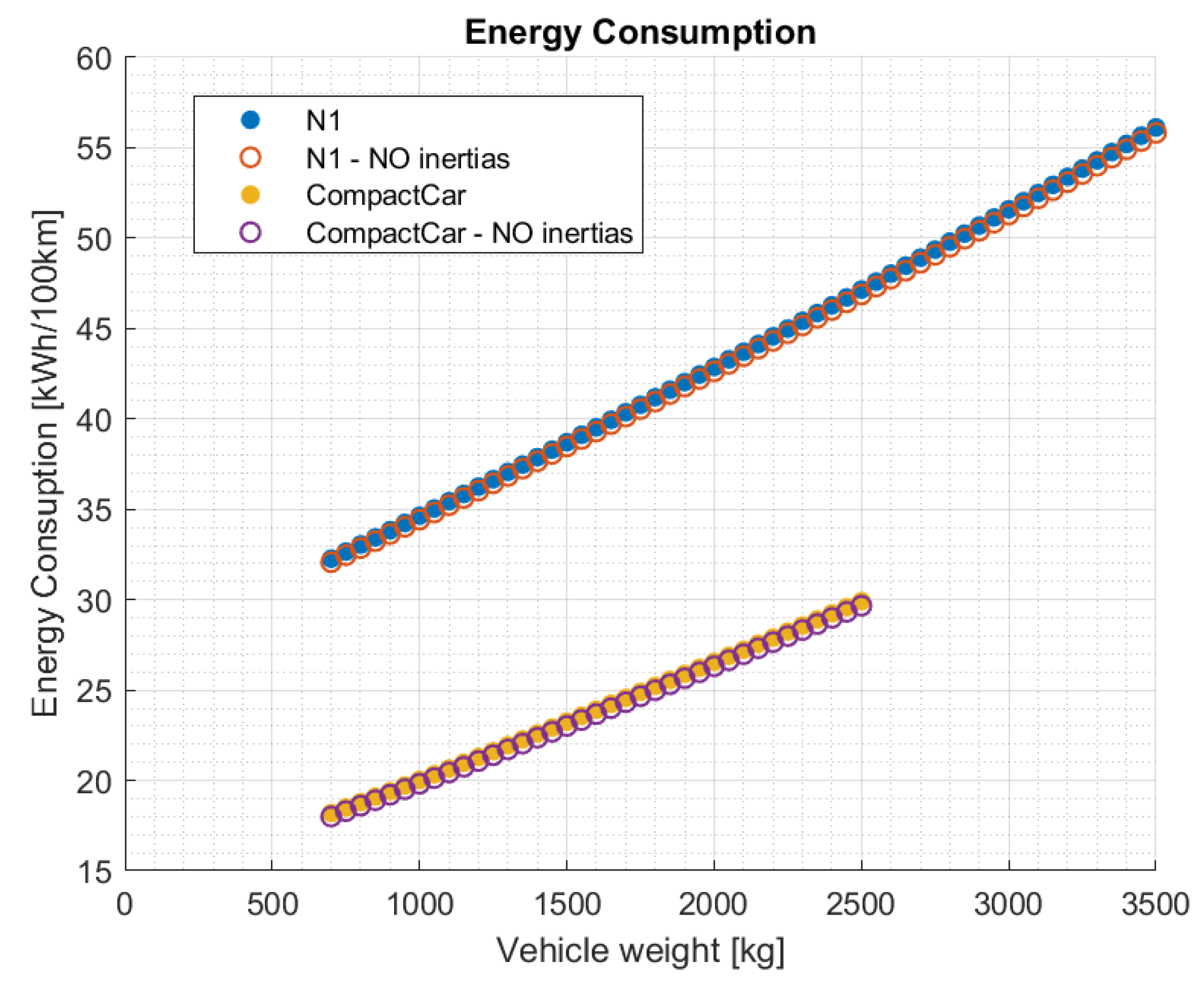
  • Inertias of the electric motor and of the rotating parts of the driveline. The contribution of the inertias appears in the equation of the resisting force, which is a function of the angular acceleration of the considered rotating component.
  • Gear ratios and wheel radius: these parameters modify the rotation speed of the various components of the driveline, at the same vehicle speed.
  • Type of battery pack, in particular the internal resistance of the cells of the pack itself.
  • Efficiencies of the transmission and the rest of the driveline (e.g., efficiency of the motor and inverter in charging and discharging).
The effect of the variation of all the parameters mentioned above is investigated below with regard to the modification to the results of a vehicle lightweighting action.

2.5. Set of Simulations

Simulations were initially carried out, using the TEST model, on the WLTC (class 3b) and US06 driving cycles, for the N1 category vehicle model and for the compact car model. These simulations were repeated, for both vehicles, setting all the inertia contributions to zero.
Further sets of simulations were also carried out, on the WLTC (class 3b) and US06 driving cycles, for the compact vehicle, in which one or more parameters of the vehicle under examination (the “CompactCar”) were replaced by the corresponding values relating to the N1 category vehicle. In fact, the contribution provided by lightweighting is often differentiated in the literature according to the vehicle class. In this study, we therefore wanted to analyze how the different parameters of the vehicle model affect the results of lightweighting in such a way as to disengage from the vehicle class and monitor which parameters lead to this differentiation.
The parameters initially chosen for comparison are the following:
  • Battery pack parameters (nominal voltage, capacity, and internal resistance);
  • Aerodynamics (Af ∙ Cx, where Af is the frontal area of the vehicle, and Cx is the longitudinal aerodynamic coefficient);
  • Efficiency of the transmission;
  • Rolling resistance (in particular, in the reference models, this resistance is a function of a rolling friction coefficient. The analysis therefore focuses on the value of this coefficient).
The investigation on the WLTC and US06 cycles was further deepened thanks to simulation sets with the following vehicle models:
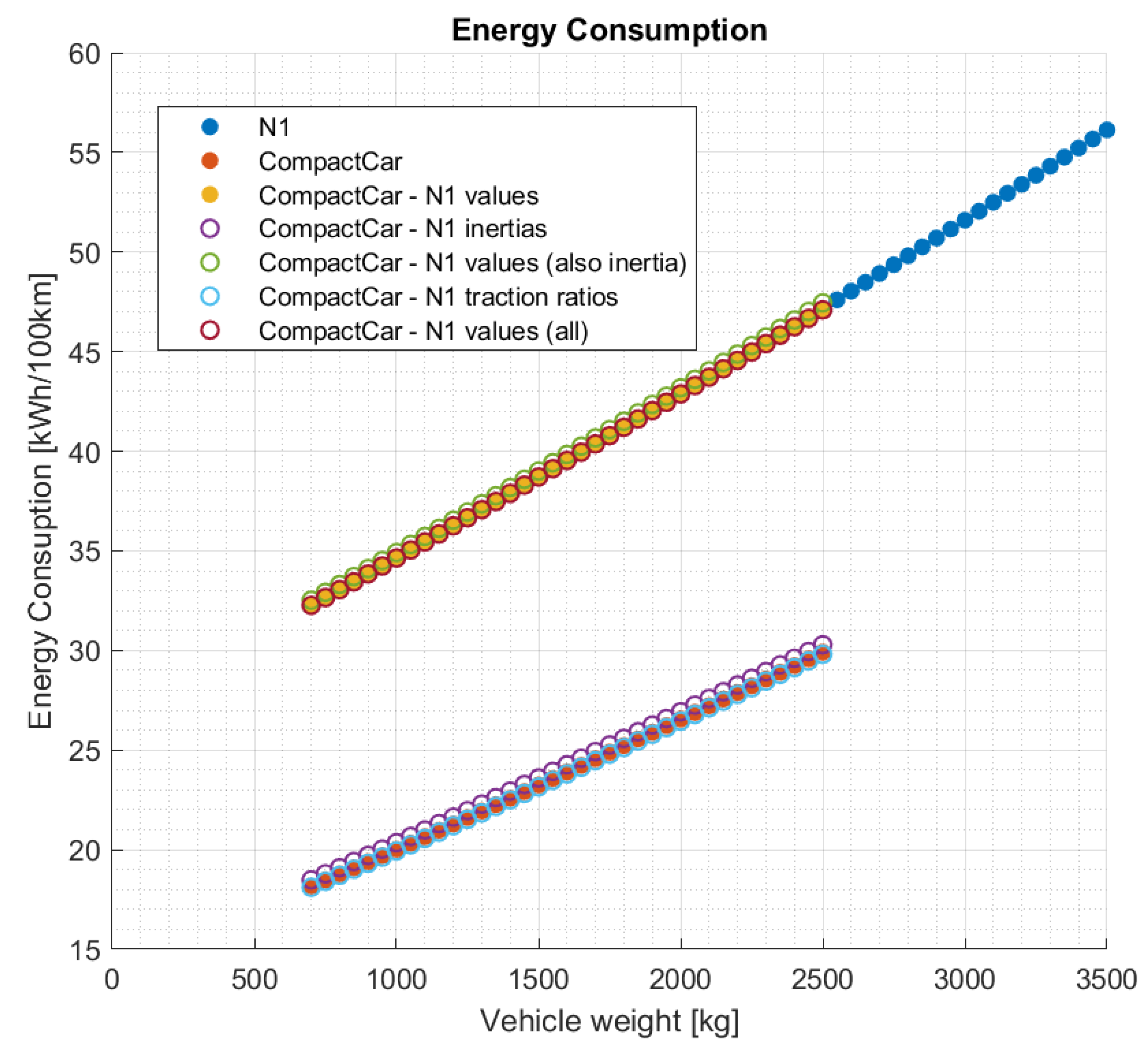
  • Compact car with the moments of inertia of the N1 vehicle;
  • Compact car with all previously listed parameters and moments of inertia of the N1 vehicle;
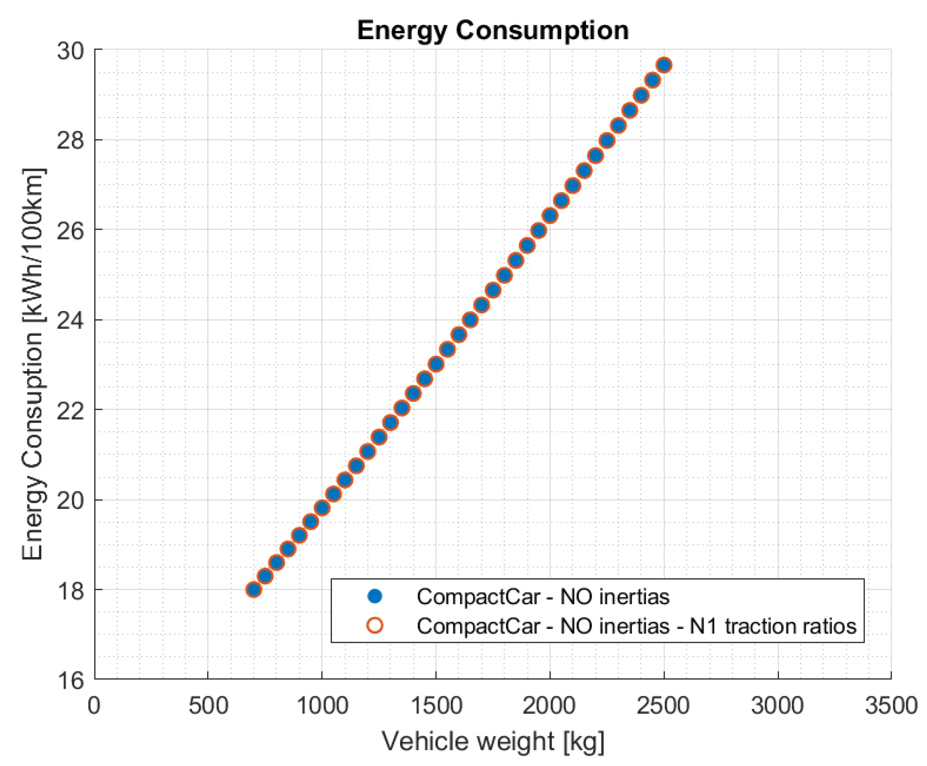
  • Compact car with the total traction ratio and wheel radii of the N1 vehicle;
  • Compact car with all previously listed parameters, moments of inertia, traction ratio, and wheel radii of the N1 vehicle.
Thanks to all the previous simulations mentioned, it was possible to define how, for a better analysis, it is more sensible to analyze the results of lightweighting for vehicle models without regenerative braking. In fact, the regenerative braking defined in Section 2.1 leads to a different entity for the regenerative recoveries according to the different transmission ratios. This aspect will be better explained in Section 3.1. All the previously presented simulations were therefore also repeated for the same vehicle models but without regenerative braking.
All previous simulations were performed for a vehicle weight of 700 to 3500 kg for the N1 vehicle and 700 to 2500 kg for the compact car. This is in order to be able to analyze the behavior over the widest possible weight range, thus also analyzing 700 kg as an extreme case with regard to the compact car. In this way, any lightening considered is certainly included in the range analyzed in this paper. A study was also carried out for the N1 vehicle assuming lightening up to a vehicle weight of 700 kg, so as to be able to make a comparison with the results obtained for the compact car.
Finally, additional sets of simulations were carried out for the N1 vehicle and the compact car model under the conditions of an absence of regenerative recovery, on further regulated driving cycles: FTP75; HWFET; JC08; and the Artemis Urban, Rural Road, and Motorway (130) Cycle [57].
For the compact car, and for the simulations on the further driving cycles, a weight range from 700 to 2500 kg was considered. For the N1 category vehicle, however, it was considered sufficient to restrict the weight range to 1100 kg to 3500 kg.

3. Results

This section shows the results of the simulations carried out, obtaining the appropriate considerations.

3.1. Benchmark Regenerative Braking Logic

For the WLTC cycle, a set of simulations was carried out for the N1 category vehicle and with the same vehicle, but setting all the inertia contributions equal to zero, to see if the inertia is negligible for the consumption analysis and, in particular, for a study on lightweighting. The same process was conducted with regards to the compact car model.
Figure 1 shows the results of the simulation sets described above, in particular, in terms of average energy consumption over the WLTC cycle, class 3b, as a function of vehicle weight.
From Figure 1, it can be seen how the inertia can be considered negligible for the study in question.
In particular, in the TEST model [48], the inertia contributions given by the wheels, by the electric motor and by the rotating parts in input and in output to the motor reducer, have been implemented. The resistive force, due to the inertia of each wheel, is calculated by multiplying the moment of inertia of the wheel by the angular velocity variation of the wheel and finally dividing this by the wheel radius. Similarly, the resistant torques, due to the inertia of the motor and of the other rotating parts, are calculated by multiplying the relative moment of inertia by the relative variation of angular speed.
During several projects undertaken by our research team, including the validation phase of the TEST model [48], it was observed that these inertia contributions are generally negligible. Therefore, even by varying the transmission ratio of the vehicle, which modifies the angular speeds, these contributions tend to remain negligible.
Other sets of simulations were also carried out for the compact car, in which the parameters of only one aspect among those mentioned in Section 2.5 “Sets of simulations” were varied, setting the relative parameters equal to those of the N1 category vehicle. These values, relating to the N1 category vehicle, have also all been set simultaneously in the “CompactCar” model to obtain a further set of simulations. The results of all these simulations, in terms of the average energy consumption of the WLTC (class 3b) cycle, as a function of the weight of the vehicle, are shown in Figure 2, together with the results of the simulations carried out for the N1 category vehicle, so as to be able to make a comparison.
From Figure 2, the aspect that least affects consumption is the battery pack, followed by the efficiency of the transmission. The parameter that has the greatest influence is aerodynamics, followed by the rolling resistance coefficient.
In particular, the contribution given by aerodynamics significantly affects the increase in vehicle consumption, but, as we will see better below, it does not involve a particular variation of the slope of the original curve given by the results of the simulations on the “CompactCar” model. The other three components (rolling resistance, transmission efficiency, and battery pack) instead involve, in addition to an increase in consumption, also a variation in the slope of the curve relating to the original compact car model.
If the four aspects considered were actually the only ones to substantially act on the effects of lightweighting, one should expect a curve relating to the set of simulations with the compact car model, but with all the parameters mentioned above equal to those of the N1 category vehicle superimposed on the curve obtained by means of the set of simulations with the N1 vehicle model itself. What has been obtained (see Figure 2) does not perfectly reflect what has just been described. In particular, the two curves overlap well for a vehicle weight range between approximately 700 and 1000 kg. Above 1000 kg, the values of the two curves begin to diverge more and more as the mass increases. The two curves therefore have two different slopes. Therefore, a further aspect or parameter that justifies this behavior must be sought.
With the sets of simulations presented in Figure 1, it can be seen that the inertias are negligible with regard to the variation in consumption; however, it is worthwhile to investigate whether the latter can instead have an influence by modifying the slope of the consumption curve according to the vehicle weight (Figure 3). Furthermore, it may also be useful to investigate the influence of the transmission ratios and wheel radii on the results since the wheel radii also act as a transmission ratio to discharge the forces to the ground (Figure 3).
From Figure 3, it can be seen that the contribution given by the moments of inertia alone is negligible as regards the average energy consumption of the WLTC cycle. The modification of the transmission ratios and of the wheel radii, equal to the values of the N1 class vehicle, instead causes a variation of the slope of the consumption curve, with a consequently more marked difference in consumption for higher vehicle weight values between the original compact car and with values of the N1 vehicle. Therefore, the transmission ratios (and the wheel radii, which also act as a transmission ratio) are also important parameters for monitoring the effects of a hypothetical lightweighting of the starting base vehicle. This can also be seen from the very good overlap of the curve of values relating to the light commercial vehicle (N1) compared to the curve relating to the compact car with the battery pack, aerodynamics, motor efficiency, rolling resistance, moments of inertia, gear ratios, and wheel radii of the N1 vehicle. All the latter aspects must therefore be taken into consideration in evaluating the benefits of lightweighting. Among all these aspects, the inertias are, in any case, the least influential and, therefore, the aspect that could possibly be neglected, as can also be seen from the graph in Figure 1.
The transmission ratios, by modifying the angular speeds of the wheels and of the various rotating parts of the transmission, cause the contribution made by the various moments of inertia to be modified. In fact, the resistant torques, due to inertia, are proportional to the moment of inertia and to the rate of change of the angular velocity of the affected component. It may be useful to investigate whether the only effect brought about by gear ratios is associated with inertias. A new set of simulations is therefore carried out, for the compact car, with all moments of inertia null and with the transmission ratios and wheel radii of the N1 vehicle, to obtain the graph shown in Figure 4.
The two curves reported in Figure 4 do not overlap. In particular, they diverge more and more as the weight of the vehicle increases. Therefore, the transmission ratios necessarily involve a further effect on consumption, in addition to that associated with inertia. It is therefore necessary to identify the reason for this further effect. To do this, the individual simulations with a vehicle weight of 2500 kg were analyzed, for the compact car without inertia and for the compact car without inertia and with the total transmission ratio (and wheel radii) of the N1 vehicle (Figure 5).
From Figure 5, it can be seen how, for the two simulations, the traction powers (or rather the discharge powers of the battery pack) are superimposed on the graph. What varies is the charging power. This aspect is due to the different contributions that regenerative braking makes according to the transmission ratios. In fact, by varying the transmission ratio, covering the same driving cycle, the angular speeds involved vary, including the angular speed of the electric motor, as can be seen from Figure 6a. In each operating point of the driving cycle under examination, thus varying the transmission ratio and in particular the angular speed of the motor, with the same power required, the motor torque varies, as can be seen from the positive values (traction motor torque) of the graph in Figure 6b. Conversely, for the braking phases, as the regenerative braking logic is set, the motor reaches a maximum value (in module) of regenerative torque with a certain ramp as a function of time. However, depending on the angular speed of the wheels (and motor), this latter torque will translate into a different power sent to the battery pack (Figure 5). Therefore, in the case of the regenerative braking logic defined as a function of time and of the maximum motor torque, with the same constant parameters of the logic (maximum torque and slope of the time–torque straight line before the plateau value), the transmission ratio will have an affect by modifying the energy recovery contribution brought about by the regenerative braking logic.
In practice, when a regenerative braking logic of the type presented in Section 2.1 is implemented in the vehicle control unit, the logic must be calibrated according to the vehicle parameters, in particular, according to the performance of the battery pack (maximum recharge power), and therefore also according to the transmission ratios. For this reason, it does not make much sense to consider two different vehicles but equipped with a regenerative braking logic characterized by the same parameters.
What has been shown in this section was also repeated for the US06 driving cycle, for which similar results and considerations were obtained.

3.2. Compact Car and N1 Vehicle in Absence of Regenerative Braking Recovery

Therefore, by varying the transmission ratios, the hypothesis according to which the vehicles are equipped with the same regenerative braking is no longer valid. The logic is in fact the same, as are the constant parameters of the logic itself, but the energy recovery is different. For this reason, to avoid dependence on this aspect, the previously presented simulations are repeated, but with the relative vehicles without regenerative braking.

3.2.1. Consumption Analysis

Figure 7 shows the results of the simulation sets described above, in particular, in terms of average energy consumption over the WLTC cycle, class 3b, as a function of vehicle weight, for vehicle N1 and for the compact car without the regenerative braking logic, with and without inertia contributions. From Figure 7, it can be seen that the inertia can be considered negligible for the study in question.
Figure 8 shows the results in terms of energy consumption on the WLTC cycle (class 3b) as a function of the vehicle weight, for the different sets of simulations, in which, for the compact car, the parameters relating to each of the aspects are considered significant, and the parameters of all aspects simultaneously are imposed, equal to the respective value of the N1 vehicle. The graph in Figure 8 also shows the results relating to the simulations carried out with the original compact car and with the N1 category vehicle.
Thanks to the analysis of the graphs shown in Figure 8, it is possible to draw the same considerations made for vehicles equipped with the regenerative braking logic (Figure 2), as regards the dependence of the four aspects considered (battery pack, aerodynamics, transmission efficiency, and rolling resistance). In the absence of regenerative braking, it is also possible to see that the correct setting of the parameters relating to the four aspects mentioned above is sufficient to correctly define the vehicle model and the related consumption in the function of the vehicle mass on the WLTC cycle (class 3b). In fact, in the graph of Figure 8, the curve relating to the compact car with the battery pack, aerodynamics, transmission efficiency, and rolling resistance parameters equal to those of the N1 vehicle matches well with the curve relating to the N1 class vehicle (both vehicles without regenerative braking). In fact, the inertia, as already defined, is negligible, and the transmission ratios (and the wheel radii) do not modify the contribution made by the regenerative braking logic, which is absent. The transmission ratios, in this case, affect only the contribution made by the inertia (see Figure 9 and Figure 10).
What has been shown in this section was also repeated for the US06 driving cycle, for which similar results and considerations were obtained.

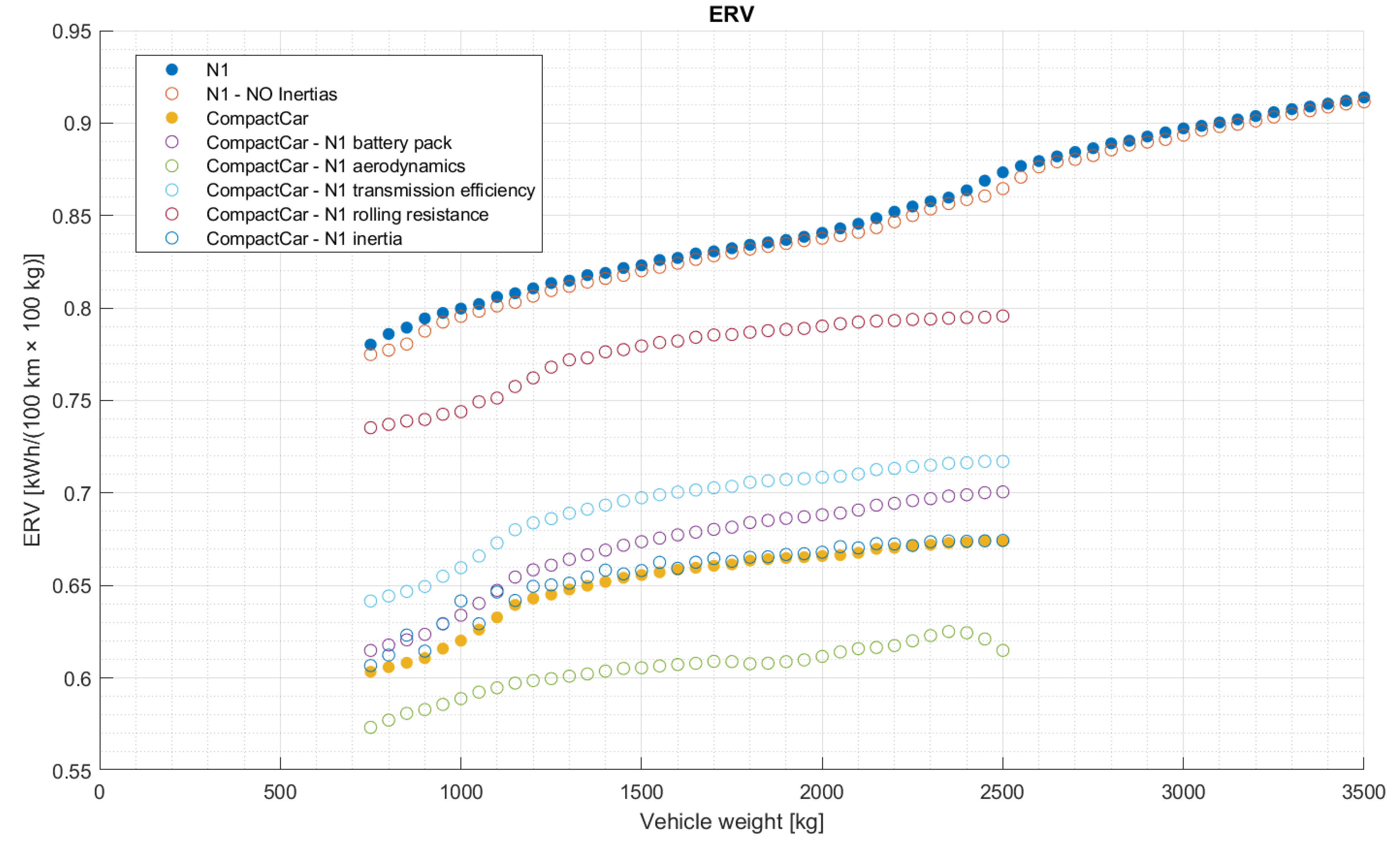
3.2.2. Polynomial Interpolation and ERV Index

In this section, we will look at the polynomial functions that best represent the curves shown previously, in Section 3.2.1. In particular, the polynomial functions of first, second, and third degree were analyzed which approximate the chosen curve, whose parameters were obtained by means of the “polyfit” function of MATLAB®.
Below, in Equation (1), the function used for polynomial interpolation is shown.
y = c 3 · x 3 + c 2 · x 2 + c 1 · x + c 0
where y is the energy consumption expressed in kWh/100 km, relating to the curve chosen for the analysis, x corresponds to the vehicle weight (in 100 kg), and c 3 , c 2 , c 1 , and c 0 are the coefficients of the polynomial, identified by the “polyfit” MATLAB function. In particular, for the first-degree polynomial, c 3 and c 2 are equal to the null value; for the second-degree polynomial, in general, only c 3 is equal to the null value; and for the third-degree polynomial, they are, in general, different, from zero to all four coefficients.
Figure 11 shows the curves, relating, respectively, to the N1 vehicle and the compact car, both without regenerative braking, obtained by means of the polynomial functions.
As can be seen from Figure 11, the third-degree and second-degree curves are those that more precisely approximate the curve of the results of the simulations carried out with the TEST model; however, even the first-degree polynomial can be useful for an analysis more approximate. The same result was also found for all the other simulations carried out in the absence of regenerative recovery (with changed parameters).
Table 2 shows the values of the coefficients of the polynomials which approximate the consumption–weight curves of the vehicle, with the coefficients obtained thanks to the “polyfit” MATLAB function. Only the coefficients relating to the first- and second-degree polynomials have been reported, since the third-degree polynomials have the negligible c 3 coefficient, which is several orders of magnitude lower than the other three coefficients, thus reducing almost to a second-degree polynomial. In fact, as can be seen from Figure 11, the second- and third-degree polynomial coincide quite well, and the curve under examination can therefore be approximated with sufficient precision simply by the second-degree polynomial. The same situation is found for the polynomials relating to the curves of all the simulations previously carried out, with vehicles without regenerative braking.
As already mentioned, in the literature, reference is often made, when calculating the energy savings associated with vehicle lightweighting, to the FRV index. Considering electric vehicles, it is better to calculate an equivalent index, the ERV index, which corresponds to the c 1 coefficient of the first-degree polynomial, shown in Table 2 for each vehicle model simulated.
Figure 12 shows the ERV index, for the WLTC cycle, calculated as in Equation (2), as a function of the vehicle weight, for vehicles without regenerative braking.
E R V i = E C i E C i 1 Δ M · 100
where E R V i , expressed in kWh 100   km · 100   kg , is the ERV index associated with the vehicle weight of the i-th simulation; E C i is the energy consumption on the WLTC cycle (class 3b), expressed in kWh 100   km , of the i-th simulation; E C i 1 is the average energy consumption of the WLTC cycle (class 3b), expressed in kWh 100   km , of the simulation with a vehicle weight immediately lower than that of the i-th simulation; and Δ M (in kg) is the mass variation of the vehicle between the i-th simulation mass and the immediately lower mass being simulated.
Also from Figure 12, it can be seen that the inertias have little influence as regards the variation of consumption and, consequently, are negligible as regards the study under examination, i.e., the evaluation of the results of the lightweighting of a vehicle. Furthermore, as could already be seen from the slight concavity of the curves presented in Figure 7, Figure 8 and Figure 10, the ERV index of the tangent line to the consumption curve increases as weight increases. This means that for greater vehicle weights, we can benefit more from lightweighting for the same weight reduction. In addition, it can be observed which parameters (if equal to those of a higher-class vehicle, class N1 for the case in question) have an effect by raising the ERV index and which by decreasing it.
Now, we carry out an energy saving analysis following a hypothetical lightweighting of a specific vehicle. The results of lightweighting are analyzed considering the ERV index, obtained as is typically performed in the literature [46], therefore as the coefficient c 1 of the first-degree polynomial (see Table 2). Furthermore, the energy consumption of the real vehicle under examination, on a reference driving cycle, for example the WLTC (class 3b), is assumed. The objective is to ascertain how an incorrect setting of the model (following the implementation of incorrect parameters) can influence the evaluation of the results of lightweighting. A considerable reduction of 300 kg is therefore considered. The compact car is considered as a “real” vehicle, assuming that its vehicle model perfectly represents a corresponding real vehicle. Finally, the ERV indices obtained by means of the c 1 coefficients of the first-degree polynomials, shown in Table 2, for the various vehicle models simulated, are considered.
Figure 13 shows the results of the 300 kg reduction, in terms of average energy consumption of the WLTC cycle (class 3b), calculated as defined above, starting from different vehicle weights.
From Figure 13, it is possible to see how the incorrect definition of the model does not cause excessive damage as regards the evaluation of the results of a lightweighting of 300 kg, provided, however, that the real consumption of the vehicle on the cycle in question is known. Furthermore, the aspects that lead to fewer errors are inertia, the battery pack, and the efficiency of the transmission. The characteristics of the vehicle and its model that most alter the results, if the study is carried out by adopting the approach described above, are instead the aerodynamics and, above all, the rolling resistance. Therefore, adopting this approach reveals a contrasting situation with respect to evaluating lightweighting considering the consumption curve obtained by means of simulations with the vehicle model. In the latter case, as observed in Figure 8, the incorrect evaluation of the rolling resistance coefficient leads to only a marginal error in the evaluation of consumption compared to an incorrect definition of aerodynamics. In fact, the increase in the aerodynamic resistance coefficient, as can be seen from Figure 8, raises the consumption curve; however, it varies the slope less than the contribution provided by the modified value of the rolling resistance coefficient.
Therefore, if we have the consumption available for the reference cycle on which we want to evaluate the results of a hypothetical lightweighting, it is convenient to use the constant ERV index approach to draw considerations close to reality. However, as an alternative, it is also possible to use the known consumptions to calibrate the vehicle model and thus obtain, through simulations, a realistic consumption curve as a function of the weight of the vehicle.
The work relating to polynomial interpolation and ERV index was also repeated for the US06 driving cycle; this led to results and considerations similar to those obtained for the WLTC cycle.

3.2.3. Comparison between Different Driving Cycles

In this section, the lightweighting results evaluated on different standardized driving cycles will be compared [61], for the N1 vehicles and for the compact car, without regenerative braking.
Figure 14 shows the average energy consumption obtained for different sets of simulations on different regulated cycles. In particular, the average energy consumption, represented by each point of the graph, corresponds to the average consumption on the cycle analyzed, obtained by carrying out a simulation with the TEST model on the cycle in question, with a pre-set weight (equal to that indicated by the abscissa axis of the graph).
From Figure 14, it is possible to observe how, as the driving cycle considered varies, the average consumption varies, as does the slope of the curves obtained and, therefore, the ERV index and the results of lightweighting. It can also be observed that one driving cycle is not more energy intensive than another in absolute terms but depends on the weight of the vehicle; in fact, for example, for the compact car, the US06 cycle is more intensive than the Artemis Motorway Cycle, for a vehicle mass greater than about 1750 kg, while it is less intensive below this weight.
From Figure 14a, it can be seen that the N1 vehicle without regenerative braking has a very similar energy consumption as the weight varies for the FTP75 and JC08 driving cycles; while for the compact car (see Figure 14b), the difference in consumption for the two cycles becomes more marked. Therefore, in addition to being dependent on the cycle considered, the difference between one cycle and another also depends on the vehicle in question.
Using the “polyfit” function of MATLAB, the polynomials of the first-, second-, and third-degree, which approximate the curves presented in Figure 14, were found. Moreover, this time, the functions which best approximate the curves are the polynomials of second and third degree, which are almost equivalent since the coefficient c 3 of the third-degree polynomial is approximately zero, while the straight line can still be significant for evaluating the results of lightweighting, in particular through its coefficient c 1 which represents the ERV index commonly used in the literature.
Table 3 and Table 4 show the coefficients of the first- and second-degree polynomials, obtained on the various standardized driving cycles, respectively, for the N1 category vehicle and for the compact car of M category (“CompactCar”).

4. Discussion

In this paper the effects of vehicle lightweighting were analyzed, in particular by monitoring which parameters of the vehicle model have the greatest influence on the results and, therefore, which must be estimated more precisely for a correct study.
In particular, the inertia contribution can be considered negligible. Furthermore, considering the consumption curve (average energy consumption vs. vehicle mass), obtained by means of simulations with a consolidated model in the literature (TEST model [48]), it was found that the aspect that least affects consumption is the battery pack, followed by the efficiency of the transmission, while the parameter that has the greatest influence is aerodynamics, followed by the rolling resistance coefficient. The contribution given by the increase in aerodynamics significantly affects the increase in vehicle consumption, but it does not involve a particular variation of the slope of the consumption curve. Moreover, by increasing all previously mentioned contributions, i.e., placing them at a value closer to that of a vehicle of a higher class, obviously, consumption increases.
Finally, for the realization of a fairly precise consumption curve, the correct setting of the battery pack parameters, aerodynamic coefficients, transmission efficiency, and rolling resistance coefficient is sufficient to correctly define the vehicle model useful for a lightweighting study and the related energy consumption in function of the vehicle mass. In fact, the inertia contribution is negligible and, in absence of the regenerative braking logic (or with an implementation of a regenerative recovery which does not depend on the transmission ratio), the transmission ratios affect only the negligible inertia contribution.
Then, the polynomials that best approximate the consumption curves identified through simulations were investigated. The third-degree and second-degree curves are those that more precisely approximate the curve of the results of the simulations carried out with the TEST model; however, even the first-degree polynomial can be useful for a more approximate analysis. In particular, for an accurate approximation, it is sufficient to consider the second-degree polynomial. In fact, the third-degree polynomials have the negligible c 3 coefficient (coefficient that multiplies the cube of the mass), several orders of magnitude lower than the other three coefficients.
In the literature, reference is often made to the FRV index, expressed in L/(100 km ∙ 100 kg), when calculating the energy savings associated with vehicle lightweighting. Considering electric vehicles, it is better to calculate an equivalent index, the ERV index, expressed in kWh/(100 km ∙ 100 kg), which approximately corresponds to the c 1 coefficient (coefficient that multiplies the mass) of the first-degree polynomial.
The real ERV increases as vehicle weight increases for the same vehicle model. This means that for greater vehicle weights, we can benefit more from lightweighting for the same weight reduction.
The inertia contribution can also be considered negligible for the calculation of the ERV index. Furthermore, considering the ERV index for evaluating the results of a hypothetical vehicle lightweighting, knowing the real consumption of the baseline vehicle, the aspects that lead to fewer errors are the incorrect definition of the battery pack parameters and the efficiency of the transmission. The characteristics of the vehicle and its model that most alter the results, if the study is carried out by adopting the ERV approach, are instead the aerodynamics and, above all, the rolling resistance. Therefore, adopting this approach reveals a contrasting situation with respect to evaluating the lightweighting considering the consumption curve. In the latter case, the incorrect evaluation of the rolling resistance coefficient leads to only a marginal error in the evaluation of consumption compared to an incorrect definition of aerodynamics. In fact, increasing the aerodynamic resistance coefficient raises the consumption curve, but changes its slope to less than the contribution provided by the modified value of the rolling resistance coefficient. However, assuming that the real consumption of the baseline vehicle is known, it is possible to calibrate the coefficients of the model, and in particular the aerodynamic coefficients, in such a way as to obtain a more realistic consumption curve.
Therefore, having the vehicle consumption available on the reference cycle on which we want to evaluate the results of a hypothetical weight reduction, if we want to avoid calibrating the aerodynamic coefficients of the vehicle model, we should use the constant ERV index approach to draw considerations close to reality.
Figure 15 summarizes the above, presenting the ERV indices obtained on the WLTC (class 3b) driving cycle, for the different vehicle models.
Finally, an initial study was also carried out on the variability of the results of the vehicle lightweighting according to the driving cycle adopted as a reference to evaluate this result. This study will eventually be further explored in a future paper.
Figure 16 summarizes the study on the different driving cycles, presenting the ERV indices obtained for the different cycles, for the N1 category vehicle and for the compact car.
As the driving cycle considered varies, average consumption varies, but also the slope of the curves obtained and, therefore, the ERV index and the results of lightweighting. It has also been observed that one driving cycle is not more energy intensive than another in absolute terms but depends on the weight of the vehicle; in fact, for example, for the compact car, the object of this study (without regenerative braking), the US06 cycle is more intensive than the Artemis Motorway Cycle for a vehicle mass greater than about 1750 kg, while it is less intensive below this weight. Furthermore, the N1 vehicle considered, without regenerative braking, has a very similar energy consumption as the weight varies for the FTP75 and JC08 driving cycles, while for the compact car, the difference in consumption for the two cycles becomes more marked. Therefore, in addition to being dependent on the cycle considered, the difference between one cycle and another also depends on the vehicle in question.
By means of the information obtained in the work presented in this paper, it is possible to obtain guidelines for the preparation of an effective vehicle model for the evaluation of lightweighting.
In future work, what is presented in this paper will be taken into account, and in particular, the influence on the results of lightweighting of the different parameters of the vehicle model, to build a database of models of electric vehicles of different classes, will be used it to calculate the relative ERV indices. The material obtained with this last work will then be used for the evaluation of the lightweighting obtained by means of various technologies, currently in the research phase at the University of Brescia.

5. Conclusions

In the literature, reference is often made to the FRV index, expressed in L/(100 km ∙ 100 kg), when calculating the energy savings associated with vehicle lightweighting. Considering electric vehicles, it is better to calculate an equivalent index, the ERV index, expressed in kWh/(100 km ∙ 100 kg). The real ERV, for the same vehicle model, increases as vehicle weight increases. This means that for greater vehicle weights, we can benefit more from lightweighting, for the same weight reduction. However, considering a constant ERV as the mass varies is, in any case, a good approximation for the same vehicle model.
In this work, it has been found that, for a correct calculation of the ERV index, it is important to establish the correct definition of the rolling resistance coefficient, followed by the aerodynamics, and then the battery pack parameters and the transmission efficiency. On the other hand, the inertia contribution can be considered negligible.
In general, for the realization of a fairly precise consumption curve, the correct setting of the battery pack parameters, aerodynamic coefficients, transmission efficiency, and rolling resistance coefficient are sufficient to correctly define the vehicle model useful for a lightweighting study and the related energy consumption in the function of the vehicle mass.
This work does not contribute to the creation of the databases of two vehicles but in the identification of the parameters that most influence the results of lightening, by means of an analytical method.
So, this work allows us to lay the foundations and guidelines for the identification of a vehicle model that reflects reality, as regards the evaluation of the results of lightweighting.
In fact, apparently, there is no similar study in the literature. Some works calculate the FRV [5,6,34,43,44,45] and ERV [45,46] indices for different vehicles, in particular within various vehicle categories (e.g., A/B, C, and D classes). The work we propose is instead the first that observes, in more detail, what are the parameters that influence the variability of the results of vehicle lightweighting. This aspect is precisely the novelty of the proposed work.
A future project will consist precisely in the creation of a database of vehicles of different classes and, if possible, the obtained databases will be validated experimentally, also experimentally validating the truthfulness of the considerations obtained in the work proposed in this paper.

Author Contributions

Conceptualization, G.S., M.G. and D.C.; methodology, G.S.; software, G.S.; formal analysis, G.S., M.G., D.C. and A.C.; data curation, G.S., A.C. and P.M.; writing—original draft preparation, G.S., M.G. and A.C.; writing—review and editing, G.S., M.G., D.C. and A.C.; visualization, M.G. and D.C.; supervision, M.G. and D.C. All authors have read and agreed to the published version of the manuscript.

Funding

This research is funded by the European Union, NextGenerationEU, see below.

Data Availability Statement

The data presented in this study are available on request from the corresponding author. The data are not publicly available due to the University of Brescia’s privacy policy.

Acknowledgments

This study was financed by the European Union—NextGenerationEU (National Sustainable Mobility Center CN00000023, Italian Ministry of University and Research Decree n. 1033—17/06/2022, Spoke 11—Innovative Materials & Lightweighting). The opinions expressed are those of the authors only and should not be considered as representative of the European Union or the European Commission’s official position. Neither the European Union nor the European Commission can be held responsible for them. CUP D83C22000690001.

Conflicts of Interest

The authors declare no conflict of interest.

Nomenclature

AbbreviationDescription
AfFrontal area of the vehicle
c 3 ,   c 2 ,   c 1 ,   c 0 y polynomial
CxLongitudinal aerodynamic coefficient (drag)
E C i Average energy consumption of the i-th simulation
E C i 1 Average energy consumption of the simulation with vehicle weight immediately lower than that of the i-th simulation
EPAU.S. Environmental Protection Agency
ERVEnergy Reduction Value
E R V i ERV index associated with the vehicle weight of the i-th simulation
EVElectric Vehicle
FRVFuel Reduction Value
FTP75Standard driving cycle (FTP75) described in the EPA Federal Test Procedure (FTP)
HWFETEPA Highway Fuel Economy Cycle
ICEVInternal Combustion Engine Vehicle
JC08Japanese Emission Test Cycle
RESInternal resistance of the battery pack
SFTPEPA Supplemental Federal Test Procedure
SFTP-US06Standard driving cycle (US06) described in the EPA Supplemental Federal Test Procedure (SFTP)
TESTTarget-speed EV Simulation Tool
WLTCWorldwide Harmonized Light-Duty Vehicles Test Cycle
WLTPWorldwide Harmonized Light-Duty Vehicles Test Procedure
x Vehicle weight (expressed in 100 kg)
y Polynomial interpolation function, energy consumption expressed in kWh/(100 km)
Δ M Vehicle mass variation between the i-th simulation and the immediately lower mass being simulated

References

  1. European Council; Council of the European Union. Stricter CO2 Emission Standards for Cars and Vans Signed Off by the Council. Available online: https://www.consilium.europa.eu/en/press/press-releases/2019/04/15/stricter-co2-emissionstandards-for-cars-and-vans-signed-off-by-the-council/ (accessed on 30 August 2022).
  2. European Law Brussels. PE-CONS 6/19. Regulation of the European Parliament and of the Council Setting CO2 Emission Performance Standards for New Passenger Cars and for New Light Commercial Vehicles, and Repealing Regulations (EC) No 443/2009 and (EU) No 510/2011 (Recast); 3 April 2019. Available online: https://www.reteambiente.it/repository/normativa/32865_final.pdf (accessed on 18 June 2023).
  3. Ehsani, M.; Gao, Y.; Longo, S.; Ebrahimi, K. Modern Electric, Hybrid Electric, and Fuel Cell Vehicles; CRC Press, Taylor & Francis Group: Boca Raton, FL, USA, 2018; pp. 1–11. [Google Scholar]
  4. Lewis, G.M.; Buchanan, C.A.; Jhaveri, K.D.; Sullivan, J.L.; Kelly, J.C.; Das, S.; Taub, A.I.; Keoleian, G.A. Green Principles for Vehicle Lightweighting. Environ. Sci. Technol. 2019, 53, 4063–4077. [Google Scholar] [CrossRef] [PubMed]
  5. Koffler, C.; Rohde-Brandenburger, K. On the Calculation of Fuel Savings through Lightweight Design in Automotive Life Cycle Assessments. Int. J. Life Cycle Assess. 2010, 15, 128–135. [Google Scholar] [CrossRef]
  6. Kim, H.C.; Wallington, T.J. Life Cycle Assessment of Vehicle Lightweighting: A Physics-Based Model to Estimate Use-Phase Fuel Consumption of Electrified Vehicles. Environ. Sci. Technol. 2016, 50, 11226–11233. [Google Scholar] [CrossRef]
  7. Ross, M. Fuel Efficiency and the Physics of Automobiles. Contemp. Phys. 1997, 38, 381–394. [Google Scholar] [CrossRef]
  8. Sullivan, J.L.; Lewis, G.M.; Keoleian, G.A. Effect of Mass on Multimodal Fuel Consumption in Moving People and Freight in the U.S. Transp. Res. D Transp. Environ. 2018, 63, 786–808. [Google Scholar] [CrossRef]
  9. Sovran, G.; Blaser, D. Quantifying the Potential Impacts of Regenerative Braking on a Vehicle’s Tractive-Fuel Consumption for the U.S., European, and Japanese Driving Schedules; SAE Technical Paper; SAE International: Warrendale, PA, USA, 2006. [Google Scholar] [CrossRef]
  10. Spreafico, C. Can Modified Components Make Cars Greener? A Life Cycle Assessment. J. Clean. Prod. 2021, 307, 127190. [Google Scholar] [CrossRef]
  11. Ford Motor Company. Sustainability Report 2016/2017; Ford Motor Company: Dearborn, MI, USA, 2017. [Google Scholar]
  12. Cheah, L.; Heywood, J. Meeting U.S. Passenger Vehicle Fuel Economy Standards in 2016 and Beyond. Energy Policy 2011, 39, 454–466. [Google Scholar] [CrossRef]
  13. Kasseris, E.P.; Heywood, J.B. Comparative Analysis of Automotive Powertrain Choices for the Next 25 Years. J. Mater. Manuf. 2007, 116, 626–647. [Google Scholar]
  14. Sperling, D.; Cannon, J.S. (Eds.) Reducing Climate Impacts in the Transportation Sector, 2009th ed.; Springer: Dordrecht, The Netherlands, 2009. [Google Scholar]
  15. Lee, W.; Schubert, E.; Li, Y.; Li, S.; Bobba, D.; Sarlioglu, B. Overview of Electric Turbocharger and Supercharger for Downsized Internal Combustion Engines. IEEE Trans. Transp. Electrif. 2017, 3, 36–47. [Google Scholar] [CrossRef]
  16. Dhana Raju, V.; Kishore, P.S.; Yamini, K. Experimental Studies on Four Stroke Diesel Engine Fuelled with Tamarind Seed Oil as Potential Alternate Fuel for Sustainable Green Environment. Eur. J. Sustain. Dev. Res. 2018, 2, 10. [Google Scholar] [CrossRef] [Green Version]
  17. Delogu, M.; Zanchi, L.; Dattilo, C.A.; Pierini, M. Innovative Composites and Hybrid Materials for Electric Vehicles Lightweight Design in a Sustainability Perspective. Mater. Today Commun. 2017, 13, 192–209. [Google Scholar] [CrossRef]
  18. MacKenzie, D.; Zoepf, S.; Heywood, J. Determinants of US Passenger Car Weight. Int. J. Veh. Des. 2014, 65, 73. [Google Scholar] [CrossRef]
  19. Kim, H.C.; Wallington, T.J. Life-Cycle Energy and Greenhouse Gas Emission Benefits of Lightweighting in Automobiles: Review and Harmonization. Environ. Sci. Technol. 2013, 47, 6089–6097. [Google Scholar] [CrossRef] [PubMed]
  20. Helms, H.; Lambrecht, U. The Potential Contribution of Light-Weighting to Reduce Transport Energy Consumption. Int. J. Life Cycle Assess. 2007, 12, 58–64. [Google Scholar]
  21. Fang, Y. Connected Vehicles Make Transportation Faster, Safer, Smarter, and Greener! IEEE Trans. Veh. Technol. 2015, 64, 5409–5410. [Google Scholar] [CrossRef]
  22. Raji, R.A.; Mohd Rashid, S.; Mohd Ishak, S. Consumer-Based Brand Equity (CBBE) and the Role of Social Media Communications: Qualitative Findings from the Malaysian Automotive Industry. J. Mark. Commun. 2019, 25, 511–534. [Google Scholar] [CrossRef]
  23. Iqbal, A.; Rehman, Z.U.; Ali, S.; Ullah, K.; Ghani, U. Road Traffic Accident Analysis and Identification of Black Spot Locations on Highway. Civ. Eng. J. 2020, 6, 2448–2456. [Google Scholar] [CrossRef]
  24. Legislative Observatory—European Parliament. 2021/0197(COD)-CO2 Emission Standards for Cars and Vans. 2023. Available online: https://oeil.secure.europarl.europa.eu/oeil/popups/printficheglobal.pdf?id=728320&l=en (accessed on 15 June 2023).
  25. Caffrey, C.; Bolon, K.; Kolwich, G.; Johnston, R.; Shaw, T. Cost-Effectiveness of a Lightweight Design for 2020–2025: An Assessment of a Light-Duty Pickup Truck; SAE Technical Paper; SAE International: Warrendale, PA, USA, 2015. [Google Scholar] [CrossRef] [Green Version]
  26. Kollamthodi, S.; Kay, D.; Skinner, I.; Dun, C.; Hausberger, S. The Potential for Mass Reduction of Passenger Cars and Light Commercial Vehicles in Relation to Future CO2 Regulatory Requirements. 2015. Available online: https://climate.ec.europa.eu/system/files/2016-11/ldv_downweighting_co2_appendices_en.pdf (accessed on 18 June 2023).
  27. Lutsey, N. Review of Technical Literature and Trends Related to Automobile Mass-Reduction Technology; UCD-ITS-RR-10-10; Institute of Transportation Studies, University of California: Davis, CA, USA, 2010. [Google Scholar]
  28. Giordano, G. Plastics Power a New Generation of Electric Vehicles. Plast. Eng. 2019, 75, 24–33. [Google Scholar] [CrossRef]
  29. Osborne, J.; FEATURE: Light Speed—How Electric Cars Are Driving a New Wave of Lightweighting. Institution of Mechanical Engineers. Available online: https://www.imeche.org/news/news-article/feature-light-speed-how-electric-cars-are-driving-a-new-wave-of-lightweighting (accessed on 14 November 2022).
  30. Alonso, E.; Lee, T.M.; Bjelkengren, C.; Roth, R.; Kirchain, R.E. Evaluating the Potential for Secondary Mass Savings in Vehicle Lightweighting. Environ. Sci. Technol. 2012, 46, 2893–2901. [Google Scholar] [CrossRef]
  31. Verbrugge, M.; Lee, T.; Krajewski, P.E.; Sachdev, A.K.; Bjelkengren, C.; Roth, R.; Kirchain, R. Mass Decompounding and Vehicle Lightweighting. Mater. Sci. Forum 2009, 618–619, 411–418. [Google Scholar] [CrossRef]
  32. Kelly, J.C.; Sullivan, J.L.; Burnham, A.; Elgowainy, A. Impacts of Vehicle Weight Reduction via Material Substitution on Life-Cycle Greenhouse Gas Emissions. Environ. Sci. Technol. 2015, 49, 12535–12542. [Google Scholar] [CrossRef] [PubMed]
  33. Hottle, T.; Caffrey, C.; McDonald, J.; Dodder, R. Critical Factors Affecting Life Cycle Assessments of Material Choice for Vehicle Mass Reduction. Transp. Res. D Transp. Environ. 2017, 56, 241–257. [Google Scholar] [CrossRef] [PubMed]
  34. Kim, H.C.; Wallington, T.J.; Sullivan, J.L.; Keoleian, G.A. Life Cycle Assessment of Vehicle Lightweighting: Novel Mathematical Methods to Estimate Use-Phase Fuel Consumption. Environ. Sci. Technol. 2015, 49, 10209–10216. [Google Scholar] [CrossRef]
  35. Akhshik, M.; Panthapulakkal, S.; Tjong, J.; Sain, M. Life Cycle Assessment and Cost Analysis of Hybrid Fiber-Reinforced Engine Beauty Cover in Comparison with Glass Fiber-Reinforced Counterpart. Environ. Impact. Assess. Rev. 2017, 65, 111–117. [Google Scholar] [CrossRef]
  36. Leduc, G.; Mongelli, I.; Uihlein, A.; Nemry, F. How Can Our Cars Become Less Polluting? An Assessment of the Environmental Improvement Potential of Cars. Transp. Policy 2010, 17, 409–419. [Google Scholar] [CrossRef]
  37. Villanueva-Rey, P.; Belo, S.; Quinteiro, P.; Arroja, L.; Dias, A.C. Wiring in the Automobile Industry: Life Cycle Assessment of an Innovative Cable Solution. J. Clean. Prod. 2018, 204, 237–246. [Google Scholar] [CrossRef]
  38. Copper Tin–CuSn—Innovative Conductor Material for Low Current and Signal Cables. Available online: https://publications.leoni.com/fileadmin/automotive_cables/publications/data_sheet/copper_thin.pdf?1475650458 (accessed on 15 June 2023).
  39. Czerwinski, F. Current Trends in Automotive Lightweighting Strategies and Materials. Materials 2021, 14, 6631. [Google Scholar] [CrossRef]
  40. Badino, V.; Baldo, G.L. LCA: Istruzioni per l’uso (LCA: Instructions for Use); Progetto Leonardo, Esculapio Editore: Bologna, Italy, 1998. [Google Scholar]
  41. van den Berg, N.W.; Dutilh, C.E.; Huppes, G. Beginning LCA—A Guide into Environmental Life Cycle Assessment; Centrum voor Milieukunde, NOH National Reuse of Waste Research Programme: Leiden, The Netherlands, 1995. [Google Scholar]
  42. Sandrini, G.; Có, B.; Tomasoni, G.; Gadola, M.; Chindamo, D. The Environmental Performance of Traction Batteries for Electric Vehicles from a Life Cycle Perspective. Environ. Clim. Technol. 2021, 25, 700–716. [Google Scholar] [CrossRef]
  43. Del Pero, F.; Delogu, M.; Pierini, M. The Effect of Lightweighting in Automotive LCA Perspective: Estimation of Mass-Induced Fuel Consumption Reduction for Gasoline Turbocharged Vehicles. J. Clean. Prod. 2017, 154, 566–577. [Google Scholar] [CrossRef]
  44. Delogu, M.; Del Pero, F.; Pierini, M. Lightweight Design Solutions in the Automotive Field: Environmental Modelling Based on Fuel Reduction Value Applied to Diesel Turbocharged Vehicles. Sustainability 2016, 8, 1167. [Google Scholar] [CrossRef] [Green Version]
  45. Del Pero, F.; Delogu, M.; Berzi, L.; Dattilo, C.A.; Zonfrillo, G.; Pierini, M. Sustainability Assessment for Different Design Solutions within the Automotive Field. Procedia Struct. Integr. 2019, 24, 906–925. [Google Scholar] [CrossRef]
  46. Del Pero, F.; Berzi, L.; Antonacci, A.; Delogu, M. Automotive Lightweight Design: Simulation Modeling of Mass-Related Consumption for Electric Vehicles. Machines 2020, 8, 51. [Google Scholar] [CrossRef]
  47. United Nations. Consolidated Resolution on the Construction of Vehicles (R.E.3); United Nations, Economic and Social Council: New York, NY, USA, 2011; Available online: https://unece.org/fileadmin/DAM/trans/doc/2017/wp29/ECE-TRANS-WP.29-1135e.docx (accessed on 15 June 2023).
  48. Sandrini, G.; Gadola, M.; Chindamo, D. Longitudinal Dynamics Simulation Tool for Hybrid Apu and Full Electric Vehicle. Energies 2021, 14, 1207. [Google Scholar] [CrossRef]
  49. Sandrini, G.; Chindamo, D.; Gadola, M. Regenerative Braking Logic That Maximizes Energy Recovery Ensuring the Vehicle Stability. Energies 2022, 15, 5846. [Google Scholar] [CrossRef]
  50. Zecchi, L.; Sandrini, G.; Gadola, M.; Chindamo, D. Modeling of a Hybrid Fuel Cell Powertrain with Power Split Logic for Onboard Energy Management Using a Longitudinal Dynamics Simulation Tool. Energies 2022, 15, 6228. [Google Scholar] [CrossRef]
  51. Electric Vehicle Database—Fiat 500e Hatchback 42 KWh. Available online: https://ev-database.org/car/1285/Fiat-500e-Hatchback-42-kWh (accessed on 23 January 2023).
  52. FleetNews Electric Car and van Data—Fiat 500e Hatchback 42 KWh Price and Specifications. Available online: https://www.fleetnews.co.uk/electric-fleet/electric-car-and-van-data/fiat/500e-1285 (accessed on 23 January 2023).
  53. COMMISSION REGULATION (EU) 2017/1151. Available online: https://unece.org/DAM/trans/doc/2018/wp29other/EU_2017_1151.pdf (accessed on 15 June 2023).
  54. EPA—United States Environmental Protection Agency. EPA US06 or Supplemental Federal Test Procedure (SFTP); EPA: Washington, DC, USA, 2023. [Google Scholar]
  55. EPA—United States Environmental Protection Agency. EPA Federal Test Procedure (FTP). Available online: https://www.epa.gov/emission-standards-reference-guide/epa-federal-test-procedure-ftp (accessed on 2 May 2023).
  56. Japan Inspection Organization—Certification and Inspection Agency in Japan Japanese JC08 Emission Test Cycle. Available online: https://japaninspection.org/japanese-jc08-emission-test-cycle/ (accessed on 2 May 2023).
  57. IMEE. Standardized Drive Cycles. Available online: https://imee.pl/pub/drive-cycles (accessed on 2 May 2023).
  58. Chindamo, D.; Gadola, M.; Romano, M. Simulation Tool for Optimization and Performance Prediction of a Generic Hybrid Electric Series Powertrain. Int. J. Automot. Technol. 2014, 15, 135–144. [Google Scholar] [CrossRef]
  59. Chindamo, D.; Economou, J.T.; Gadola, M.; Knowles, K. A Neurofuzzy-Controlled Power Management Strategy for a Series Hybrid Electric Vehicle. Proc. Inst. Mech. Eng. Part D: J. Automob. Eng. 2014, 228, 1034–1050. [Google Scholar] [CrossRef]
  60. Sandrini, G.; Gadola, M.; Chindamo, D.; Zecchi, L. Model of a Hybrid Electric Vehicle Equipped with Solid Oxide Fuel Cells Powered by Biomethane. Energies 2023, 16, 4918. [Google Scholar] [CrossRef]
  61. Chindamo, D.; Gadola, M. What Is the Most Representative Standard Driving Cycle to Estimate Diesel Emissions of a Light Commercial Vehicle? IFAC-PapersOnLine 2018, 51, 73–78. [Google Scholar] [CrossRef]
Figure 1. Average energy consumption of the WLTC cycle (class 3b), as a function of vehicle weight for the N1 category vehicle model (“N1”) and for the same model, but with zero inertia contributions (“N1—NO inertias”); for the compact vehicle model (“CompactCar”) and for the same model, but with zero inertia contributions (“CompactCar—NO inertias”).
Energies 16 05157 g001
Figure 2. Average energy consumption of the WLTC cycle (class 3b), as a function of vehicle weight, for the following vehicle models: vehicle of N1 category (“N1”), compact car (“CompactCar”); compact car with the N1 battery pack on board (“CompactCar—N1 battery pack”); compact car with the aerodynamic coefficients of the N1 vehicle (“CompactCar—N1 aerodynamics”); compact car with transmission efficiency equal to that of the N1 vehicle (“CompactCar—N1 transmission efficiency”); compact car with rolling resistance coefficient of N1 vehicle (“CompactCar—N1 rolling resistance”); and, finally, compact car with all the parameters previously mentioned equal to those of the N1 vehicle (“CompactCar—N1 values”).
Energies 16 05157 g002
Figure 3. Average energy consumption of the WLTC cycle (class 3b), as a function of vehicle weight, for the following vehicle models: vehicle of N1 category (“N1”), compact car (“CompactCar”); compact car with the battery pack, with the aerodynamic coefficients, the efficiency of the transmission, and with the rolling resistance coefficient of the N1 vehicle (“CompactCar—N1 values); compact car with the same moments of inertia as vehicle N1 (“CompactCar—N1 inertias”); compact car with the battery pack, aerodynamics, transmission efficiency, rolling resistance, and moments of inertia of vehicle N1 (“CompactCar—N1 values (also inertia)”); compact car with the transmission ratios and wheel radii of the N1 vehicle (“CompactCar—N1 traction ratios”); and, finally, compact car with all the parameters related to the previously mentioned aspects equal to those of the N1 vehicle, i.e., the parameters relating to the battery pack, aerodynamics, transmission efficiency, rolling resistance, moments of inertia, transmission ratios, and wheel radii (“CompactCar—N1 values (all)”).
Energies 16 05157 g003
Figure 4. Average energy consumption of the WLTC cycle (class 3b), according to vehicle weight, for the following vehicle models: compact car with zero inertia (“CompactCar—NO inertias”); compact car with zero inertia and transmission ratios (and wheel radii) equal to those of the N1 vehicle (“CompactCar—NO inertias—N1 traction ratios”).
Energies 16 05157 g004
Figure 5. Output (positive) and input (charging, negative) power to the battery pack as a function of the simulation time, for simulations on the WLTC cycle, class 3b, of the compact car model with zero inertia (“NO inertias”) and the compact car model with zero inertia and the transmission ratios and wheel radii of the N1 vehicle (“NO inertias and N1 traction ratios”)—both models have a vehicle weight of 2500 kg.
Energies 16 05157 g005
Figure 6. (a) Motor angular speed and (b) motor torque, as a function of simulation time, for simulations on the WLTC cycle, class 3b, of the compact car with zero inertia (“NO inertias”) and the compact car with zero inertia and the transmission ratios and wheel radii of the N1 vehicle (“NO inertias and N1 traction ratios”)—both models have a vehicle weight of 2500 kg.
Energies 16 05157 g006
Figure 7. Average energy consumption of the WLTC cycle (class 3b), as a function of vehicle weight, with vehicles without regenerative braking for the N1 category vehicle model (“N1”) and for the same model, but with zero inertia contributions (“N1—NO inertias”); for the compact car model (“CompactCar”) and for the same model, but with zero inertia contributions (“CompactCar—NO inertias”).
Energies 16 05157 g007
Figure 8. Average energy consumption of the WLTC cycle (class 3b), as a function of vehicle weight, for the following vehicle models without regenerative braking: vehicle of N1 category (“N1”), compact car (“CompactCar”); compact car with the N1 battery pack on board (“CompactCar—N1 battery pack”); compact car with the aerodynamic coefficients of the N1 vehicle (“CompactCar—N1 aerodynamics”); compact car with the transmission efficiency equal to that of the N1 vehicle (“CompactCar—N1 transmission efficiency”); compact car with the rolling resistance coefficient equal to that of the N1 vehicle (“CompactCar—N1 rolling resistance”); and, finally, compact car with all the parameters previously mentioned equal to those of vehicle N1 (“CompactCar—N1 values”).
Energies 16 05157 g008
Figure 9. Average energy consumption of the WLTC cycle (class 3b), according to the vehicle weight, for the following vehicle models without regenerative braking: compact car without inertia (“CompactCar—NO inertias”); compact car with transmission ratios (and wheel radii) equal to those of the N1 vehicle and without inertia (“CompactCar—NO inertias—N1 traction ratios”).
Energies 16 05157 g009
Figure 10. Average energy consumption of the WLTC cycle (class 3b), as a function of vehicle weight, for the following vehicle models without regenerative braking: vehicle of category N1 (“N1”), compact car (“CompactCar”); compact car with the battery pack of the N1 vehicle on board, with the aerodynamic coefficients, the efficiency of the transmission, and with the rolling resistance coefficient of the N1 vehicle (“CompactCar—N1 values); compact car with the same moments of inertia as vehicle N1 (“CompactCar—N1 inertias”); compact car with the battery pack, aerodynamics, transmission efficiency, rolling resistance, and moments of inertia of the N1 vehicle (“CompactCar—N1 values (also inertia)”); compact car with the transmission ratios and wheel radii of the N1 vehicle (“CompactCar—N1 traction ratios”); and, finally, compact car with all the previously mentioned parameters equal to those of the N1 vehicle, i.e., the parameters relating to the battery pack, aerodynamics, transmission efficiency, rolling resistance, moments of inertia, transmission ratios, and wheel radii (“CompactCar—N1 values (all)”).
Energies 16 05157 g010
Figure 11. Average energy consumption on WLTC cycle (class 3b), as a function of the vehicle weight, for vehicles without regenerative braking. Curves relating to the results were obtained by means of simulations (“Results”), and curves were obtained thanks to the polynomial approximation of the first (“n = 1”), second (“n = 2”), and third degree (“n = 3”) for (a) the N1 vehicle; (b) the compact car.
Energies 16 05157 g011
Figure 12. ERV index, calculated for the WLTC cycle (class 3b) and calculated between a simulation performed at a given vehicle weight and the simulation with the vehicle weight immediately lower than that under examination (considering the set of simulations performed), as a function of the vehicle weight, for the following vehicle models without regenerative braking: N1 category vehicle (“N1”); N1 vehicle with zero inertia (“N1—NO Inertias”); compact car (“CompactCar”); compact car with the N1 battery pack on board (“CompactCar—N1 battery pack”); compact car with the aerodynamic coefficients of the N1 vehicle (“CompactCar—N1 aerodynamics”); compact car with transmission efficiency equal to that of the N1 vehicle (“CompactCar—N1 transmission efficiency”); compact car with the N1 vehicle rolling resistance coefficient (“CompactCar—N1 rolling resistance”); and, finally, compact car with moments of inertia equal to those of the N1 vehicle (“CompactCar—N1 inertia”).
Energies 16 05157 g012
Figure 13. Average energy consumption of the WLTC cycle, as a function of vehicle weight, for the CompactCar without regenerative braking, obtained through simulations with the TEST model (“Real consumption”) and considering the ERV obtained for the following vehicle models without recovery regenerative braking: CompactCar (“Calculated consumption”); CompactCar with the vehicle battery pack N1 on board (“Calculated consumption (ERV with N1 battery pack)”); CompactCar with the aerodynamic coefficients of vehicle N1 (“Calculated consumption (ERV with the N1 aerodynamics)”); CompactCar with the transmission efficiency equal to that of the N1 vehicle (“Calculated consumption (ERV with N1 efficiencies)”); CompactCar with the vehicle rolling resistance coefficient N1 (“Calculated consumption (ERV with N1 rolling resistance)”); and, finally, CompactCar with moments of inertia of vehicle N1 (“Calculated consumption (ERV with N1 inertias)”).
Energies 16 05157 g013
Figure 14. Average energy consumption, for (a) the N1 category vehicle and (b) compact car, without regenerative braking, on the following standard driving cycles: WLTC (class 3b); US06; FTP75; HWFET; JC08; Artemis, Urban Cycles; Artemis, Rural Road Cycle; Artemis, Motorway Cycle (130).
Energies 16 05157 g014
Figure 15. ERV index, obtained from the “polyfit” MATLAB function, on the WLTC (class 3b) driving cycle, for the N1 vehicle, for the compact car, and for the compact car with the following parameters, aspects, and components of the N1 vehicle: aerodynamics; moments of inertia; battery pack; transmission efficiency; and rolling resistance.
Energies 16 05157 g015
Figure 16. ERV index, obtained from the “polyfit” MATLAB function, for different standard driving cycles, for the N1 vehicle and for the compact car.
Energies 16 05157 g016
Table 1. Compact car and N1 vehicle characteristics.
ParameterCompact Car ValueN1 Value
Motor power87 kW>160 kW
Vehicle weight1548.38 kg 13500 kg 2
Motor efficiency98%98% 3
Transmission efficiency10.9409
Inverter efficiency in discharge0.880.88
Inverter efficiency in charge0.80.8
Auxiliary power1500 W1500 W
Af ∙ Cx 41.034 m22.1 m2
Vertical aerodynamic coefficient−0.026 m20
Rolling friction coefficient0.010.015
Total gear ratio9.66.22
Front wheel radius0.2987 m0.35 m
Rear wheel radius0.3005 m0.35 m
Moment of inertia of the wheels0.882 kg m21.09 kg m2
Moment of inertia of the motor0.02 kg m20.086 kg m2
Moment of inertia of the transmission0.0001 kg m20.01 kg m2
Battery capacity42 kWh (105 Ah)120 Ah
Number of battery cells in series96108
Number of battery cells in parallel21
Nominal battery pack voltage400.0 V356.1 V
RES 50.086 Ω0.097 Ω
1 Empty weight. 2 Fully loaded weight. 3 The N1 vehicle considered has an efficiency map for the electric motor [48]. The mean efficiency is approximately around 98%. For simplicity, this constant value was used as an approximation. 4 Frontal area (Af) multiplied by longitudinal aerodynamic coefficients (drag, Cx). 5 Internal resistance of the battery pack.
Table 2. Coefficients of the polynomial functions that approximate the consumption curves, as a function of the vehicle weight obtained by means of simulations on the various vehicle models without regenerative braking. The items under the label “VEHICLE MODEL” refer to the polynomials that approximate the curves shown in Figure 7, Figure 8, and Figure 10 (in this table, the name associated with each vehicle model is the same shown in the legend of the graphs of these figures, with the addition of “CompactCar—N1 inertias and traction ratios”, which refers to the compact car with the inertia values, transmission ratios, and wheel radii of the N1 vehicle).
Vehicle ModelPolynomial Degree c 2 k W h 100   k m · 100   k g 2 c 1 k W h 100   k m · 100   k g c 0 k W h 100   k m
N11st degree00.85225.995
2nd degree0.00240.75026.903
N1—
NO inertias
1st degree00.84825.819
2nd degree0.00240.74626.732
CompactCar1st degree00.65413.488
2nd degree0.00180.59613.900
CompactCar—
NO inertias
1st degree00.65113.304
2nd degree0.00200.58613.766
CompactCar—
N1 battery pack
1st degree00.67313.514
2nd degree0.00220.60214.024
CompactCar—
N1 aerodynamics
1st degree00.60624.564
2nd degree0.00110.57024.817
CompactCar—
N1 transmission efficiency
1st degree00.69614.105
2nd degree0.00190.63414.547
CompactCar—
N1 rolling resistance
1st degree00.77813.597
2nd degree0.00180.72114.003
CompactCar—
N1 values
1st degree00.82626.357
2nd degree0.00190.76626.779
CompactCar—
N1 inertias
1st degree00.65813.772
2nd degree0.00150.61014.117
CompactCar—
N1 values (also inertia)
1st degree00.83026.607
2nd degree0.00180.77227.019
CompactCar—
N1 traction ratios
1st degree00.65313.411
2nd degree0.00190.59213.841
CompactCar—
N1 inertias and traction ratios
1st degree00.65413.508
2nd degree0.00180.59813.912
CompactCar—
N1 values (all)
1st degree00.82526.380
2nd degree0.00180.76926.781
Table 3. Coefficients of the polynomial functions (first and second degree) which approximate the consumption curves as a function of the vehicle weight obtained by means of simulations on the N1 category vehicle model, without regenerative braking, on the following standard driving cycles: WLTC (class 3b); US06; FTP75; HWFET; JC08; Artemis, Urban Cycles; Artemis, Rural Road Cycle; Artemis, Motorway Cycle (130).
Driving CyclePolynomial Degree c 2 k W h 100   k m · 100   k g 2 c 1 k W h 100   k m · 100   k g c 0 k W h 100   k m
WLTC—Class 3b1st degree00.85225.995
2nd degree0.00240.75026.903
US061st degree01.07734.562
2nd degree0.00610.81936.855
FTP751st degree00.94615.229
2nd degree0.00160.87415.972
HWFET1st degree00.63024.647
2nd degree0.00120.57725.198
JC081st degree00.94415.362
2nd degree0.00100.89715.847
Artemis—Urban Cycle1st degree01.42613.082
2nd degree0.00141.36113.759
Artemis—
Rural Road Cycle
1st degree00.92918.344
2nd degree0.00300.79319.760
Artemis—
Motorway Cycle (130)
1st degree00.83544.654
2nd degree0.00400.65146.568
Table 4. Coefficients of the polynomial functions (first and second degree) which approximate the consumption curves as a function of the vehicle weight obtained by means of simulations on the compact car model, without regenerative braking, on the following standard driving cycles: WLTC (class 3b); US06; FTP75; HWFET; JC08; Artemis, Urban Cycles; Artemis, Rural Road Cycle; Artemis, Motorway Cycle (130).
Driving CyclePolynomial Degree c 2 k W h 100   k m · 100   k g 2 c 1 k W h 100   k m · 100   k g c 0 k W h 100   k m
WLTC—Class 3b1st degree00.65413.488
2nd degree0.00180.59613.900
US061st degree00.80916.549
2nd degree0.00310.71117.247
FTP751st degree00.7469.742
2nd degree0.00080.7219.917
HWFET1st degree00.42612.370
2nd degree0.00080.40012.557
JC081st degree00.75410.114
2nd degree0.00080.72910.292
Artemis—Urban Cycle1st degree01.20311.528
2nd degree0.00041.18911.628
Artemis—
Rural Road Cycle
1st degree00.7239.709
2nd degree0.00220.65110.219
Artemis—
Motorway Cycle (130)
1st degree00.57720.577
2nd degree0.00300.48221.253
Disclaimer/Publisher’s Note: The statements, opinions and data contained in all publications are solely those of the individual author(s) and contributor(s) and not of MDPI and/or the editor(s). MDPI and/or the editor(s) disclaim responsibility for any injury to people or property resulting from any ideas, methods, instructions or products referred to in the content.

