Abstract
Airborne wind energy systems using flexible membrane wings have the advantages of a low weight, small packing volume, high mobility and rapid deployability. This paper investigates the aero-structural deformation of a leading edge inflatable kite for airborne wind energy harvesting. In the first step, a triangular two-plate representation of the wing is introduced, leading to an analytical description of the wing geometry depending on the symmetric actuation state. In the second step, this geometric constraint-based model is refined to a multi-segment wing representation using a particle system approach. Each wing segment consists of four point masses kept at a constant distance along the tubular frame by linear spring-damper elements. An empirical correlation is used to model the billowing of the wing’s trailing edge. The linear spring-damper elements also the model line segments of the bridle line system, with each connecting two point masses. Three line segments can also be connected by a pulley model. The aerodynamic force acting on each wing segment is determined individually using the lift equation with a constant lift coefficient. The particle system model can predict the symmetric deformation of the wing in response to a symmetric actuation of the bridle lines used for depowering the kite (i.e., changing the pitch angle). The model also reproduces the typical twist deformation of the wing in response to an asymmetric line actuation used for steering the kite. The simulated wing geometries are compared with photogrammetric information taken by the onboard video camera of the kite control unit, focusing on the wing during flight. The results demonstrate that a particle system model can accurately predict the geometry of a soft wing at a low computational cost, making it an ideal structural building block for the next generation of soft wing kite models.
1. Introduction
Airborne wind energy (AWE) systems employ tethered flying devices to harvest wind energy. The emerging technology uses up to 90% less material than conventional wind turbines [1,2] and can access thus far untapped wind resources at higher altitudes [3,4]. The most commonly pursued concept uses the pulling force of a kite flown in crosswind manoeuvres to drive a drum-generator module on the ground. Once the tether reaches its maximum length, these manoeuvres are terminated, the kite is depowered, and the tether is reeled back in, consuming some of the previously generated power. When reaching the defined minimum tether length, the kite is powered again and manoeuvered in cross-wind flight patterns while reeling out the tether. Because the reel-in phases are shorter, and the pulling force of the depowered kite is lower, this cyclic operation generates net energy.
Two types of kites are used for airborne wind energy harvesting: fixed-wing and soft wing kites. This paper is about the second type, specifically the configuration illustrated in Figure 1 with a leading edge inflatable (LEI) wing, a bridle line system and a suspended, remote-controlled cable robot, which is denoted as the kite control unit (KCU).
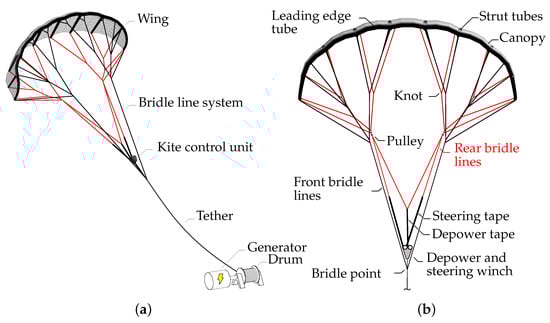
Figure 1.
Soft-wing ground-generating AWE system. (a) Complete AWE system. (b) Kite front view, adapted from [5]. The original TU Delft V3 kite is depicted, which was further developed by Kitepower B.V. [6]. The front bridle lines attached to the LE are coloured in black, while the rear bridle lines attached to the trailing edge (TE) are coloured in red.
The wing consists of an inflated tubular frame, combining a leading edge (LE) tube and several connected strut tubes, to which a fabric membrane, denoted as the canopy, is attached. The inflated tubular frame spans the wing in the spanwise and chordwise directions, transmitting the aerodynamic load generated during flight from the canopy to the bridle line system. The frame also provides the structural stability for handling the wing on the ground and during launching and landing.
Like a parafoil, a soft wing kite functions as a rotating and morphing aerodynamic control surface, actuated by the KCU via the bridle line system. The depower tape is used for symmetrically actuating the rear bridle lines, modifying the pitch of the wing relative to the KCU and, through that, the angle relative to the inflow and consequently the aerodynamic loading. Oehler and Schmehl [5] investigated the mechanism of depowering experimentally, concluding that the wing also experiences a symmetric deformation because of its C shape and bridling. Additionally, the entire kite pitches forward because of a chordwise shift of the aerodynamic centre. In some kite designs, the deformation is mitigated by integrating pulleys into the front bridle lines [7].
The steering tape is used for asymmetrically actuating the rear bridle lines, pulling in one half of the trailing edge while releasing the other half. This causes the wing to yaw, roll and twist, creating an aerodynamic side force and introducing a turning manoeuvre. The steering mechanism was investigated experimentally by Oehler et al. [8], following up on the earlier work of Breukels [9]. Using a more recent dataset of 87 automatically flown pumping cycles with high path-tracking accuracy, Roullier [10] presented an updated experimental analysis of the kite’s dynamic behaviour, with a particular focus on dynamic contributions from the suspended KCU.
Because of the curved wing shape, the actuation-induced morphing and the strong aero-structural coupling, modelling the aerodynamics of soft kites is generally more challenging than that of conventional aircraft. Point-mass models are based on simplifying assumptions for the orientation of the kite and employ constant aerodynamic coefficients [11,12]. Rigid body models include the orientation of the kite as the degree of freedom and account for the variation in the aerodynamic coefficients with the attitude in relation to the relative flow [13,14]. The point-mass and rigid body models are commonly used for estimating the performance [15] or developing the flight control algorithms [16] of AWE systems. The aerodynamic coefficients are either determined by identification from flight test data [5,10,12] or computed with simple aerodynamic models [17]. Flight test data have also been used to linearly correlate the turn rates of soft kites with the steering input [14,18,19].
Fechner et al. [20] described the rigid-body motion of a kite using an arrangement of five point masses—four to represent the wing and one for the suspended KCU—that are interconnected by relatively stiff spring-damper elements, practically acting as distance constraints. The aerodynamic force generated by the wing was calculated from three independently actuated wing segments attached to this particle cluster: the horizontal centre wing segment, producing the pulling force of the kite and modulated by changing the pitch and thus the angle of attack due to symmetric actuation, and the two vertical wing tip segments producing the side forces required for turning manoeuvres, modulated by changing the local side slip angles due to asymmetric actuation. While this five-point model does not reproduce the deformation of the kite, it does account for the effect of depowering and steering actuation on the aerodynamics.
Breukels et al. [21] developed a fluid–structure interaction (FSI) model of an LEI wing discretising the inflated tubular frame with an assembly of rigid bodies connected by universal joints and torsion springs and representing the canopy as a lattice of linear spring-damper elements. The aerodynamic load distribution was determined by partitioning the wing into spanwise segments and representing each with a discretised chordline. In the next step, the aerodynamic coefficients were evaluated at the wing section using look-up tables as functions of the chamber of the chordline, the local tube thickness and the angle of attack. The look-up tables were precomputed using 2D computational fluid dynamics (CFD). In the last step, the aerodynamic coefficients were used to recreate the pressure distribution on the wing segment. The developed FSI model can describe the symmetric and asymmetric deformation modes of the kite but comes at the additional cost of a commercial solver (MD Adams) and substantially increased computational effort.
Bosch et al. [22] combined Breukels’s aerodynamic load correlation with a finite-element (FE) model of the LEI wing using beam and shell elements. The simulations reproduced the bending and torsion deformation of the wing, but the overall accuracy was limited by the relatively low fidelity of the aerodynamic model. Geschiere [23] expanded on the approach of Bosch et al. and coupled the FSI model with a flight dynamic model to simulate flight manoeuvres for the TU Delft V3 kite. Due to lacking test flight data, it was not possible to properly validate the FSI model.
Leloup et al. [24] employed a 3D lifting line theory to determine the aerodynamic loading on the wing, considering viscous flow phenomena only in 2D using XFOIL [25]. De Solminihac et al. [26] extended this aerodynamic model to include the nonlinearity of the lift polar. The model was coupled to a structural model where beam elements represented the LE tube, leading to a kite beam model. Duport [27] compared FSI simulations using the `kite as a beam’ method to an FE method and concluded that the computational time reduction from hours to minutes was worth the marginal accuracy loss. As the model still requires calibration, it is unsuitable as a stand-alone design application.
Van Til et al. [28] proposed a soft kite model using rigid plates that are interconnected by gimbal joints and allow for rotational degrees of freedom which mimic the basic deformations of a C-shaped kite. The approach can be regarded as a further development of Fechner et al. [20], now inlcuding the bending and torsional stiffness of the three-plate wing structure as well.
The objective of this work is to develop an aero-structural deformation model of an LEI kite that can reproduce the basic deformation modes at a relatively low computational cost, preferably even faster than in real time. For validation, video footage from flight testing is analysed using a novel photogrammetry method to determine the change in the projected wing span with the symmetric actuation status of the kite. The present paper is based on the graduation project of the first author [29], which was followed up by the graduation project of Cayon [30], who introduced an improved aerodynamic model.
2. Method
The modelling approach is based on the assumption that the global geometry of the aerodynamically loaded membrane wing is governed mainly by the geometry of the bridle line system. The compressive and tensile stiffness of the tubular frame ensures that the geometric distances between the bridle line attachment points remain constant. The effect of bending and torsional stiffness on the global wing geometry is considered to be negligible and only relevant locally between the line attachments to support the canopy. The dominant role of the bridle line geometry is supported by the observation that in some flight tests with partially deflated tubular frames, the kite kept flying without a perceivable effect on the global wing geometry. Furthermore, single-skin kites function entirely without an inflated tubular frame, as pure membrane structures are tensioned solely by the aerodynamic suction pressure [31]. In the following subsections, the specific kite used in this study is detailed, two different geometric constraint-based models of this kite are proposed, and the photogrammetry technique for experimental validation is described.
2.1. Kite Specification
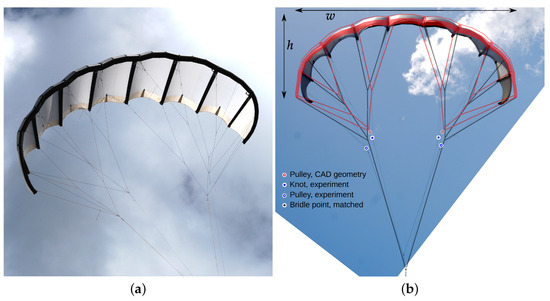
Figure 2.
TU Delft V3 kite in flight without KCU and instrumentation, manually controlled from the ground and photographed from the ground in July 2012. (a) Perspective view. (b) Rear view, showing photo overlayed with the design (CAD) geometry depicted in Figure 1b. In the photo, the positions of pulleys and knots are marked by different symbols. Scales of photo and design geometry are matched to identical heights of the kite (maximum geometric distance between bridle point and canopy).
Developed in 2012 by TU Delft researchers John van den Heuvel and Rolf van der Vlugt together with kite designer Martial Camblong, the design of this 25 m2 kite was inspired by the commercial 14 m2 kite Genetrix Hydra V4 to meet the requirements of airborne wind energy harvesting with a suspended, remote-controlled cable robot. Compared with kites commonly used for kiteboarding, the wing is relatively flat, and the bridle line system is short to facilitate launching and landing from an upside-down hanging position [32]. To achieve high wing loading and maintain good control authority, the wing is fully supported by front and rear bridle line systems. When flying crosswind manoeuvres at the nominal wind speed, the V3 kite generates an average pulling force of 3 kN, sufficient to produce shaft power of 20 kW at the ground station [12,33].
In March 2017, the TU Delft spin-off company Kitepower B.V. conducted instrumented flight tests, measuring the relative flow velocity and its direction at the kite for the first time and using this for aerodynamic characterisation [5]. The properties of the wing’s design geometry and the kite’s component masses for these tests are listed in Table 1. During flight, the wing deforms as a result of aerodynamic loading. A comparison of the deformed geometry with the designed geometry is illustrated in Figure 2b. The overlay shows how the canopy billowing between the struts reduces the distances between the strut tips. This geometric contraction of the trailing edge (TE) pulls the LE tips towards the centre of the wing. The vertical positions of the pulleys in the photo differ significantly from the positions in the overlaid CAD geometry. The reasons for this could be that the photo was not taken from the exact rear perspective and that bridle line lengths were often adjusted on the fly during flight testing to tune the flight behaviour of the kite. As part of the flight tests, the wing planform of the V3 kite was also video recorded with a camera mounted on the KCU [34]. This footage reveals that the load-induced TE contraction increases the sweep angle of the wing in flight [5].

Table 1.
Specifications of the TU Delft LEI V3 kite operated by Kitepower B.V. in March 2017 [5]. (a) Design (CAD) geometry of the wing. (b) Masses of the kite components.
2.2. Depowering and Steering Kinematics
The TU Delft V3 kite is controlled by changing the lengths of the steering and depower tapes. Because the layout of the bridle line system and the line lengths differs from kite to kite, the relative power and steering settings, and , respectively, were introduced as dimensionless input parameters for the depower and steering kinematics [14,35]. The setting refers to a fully powered kite, while refers to the depowered kite. Similarly, the setting refers to no steering input, while and 1 refer to the extreme steering inputs for right and left turns, respectively. It is assumed that the tape lengths vary linearly with the values of and .
Oehler and Schmehl [5] proposed a kinematic relation between the deployed length of the depower tape and the power setting . In the present manuscript, this relation is extended to account for different maximum depower configurations used in different flight campaigns. The deployed length of the depower tape can be defined as
where is the deployed length in the fully powered state and is the length change to fully depower the kite. The relation between this length change and the power setting is described by
where is the maximum possible length change (depending on the tape capacity of the depower winch) and is a factor between 0 and 1 quantifying how much of this maximum possible length change was actually used during the flight campaign. The variable upper limit of the deployed depower tape was introduced in the present work because kites are commonly designed for high performance when powered, while the optimal rear bridle line extension to achieve the desired depower state is determined by flight testing as a trade-off with flight stability, safety and controllability.
The deployed lengths of the left and right steering tapes can be defined as follows
where is the deployed length of both tapes in straight flight without any steering input and is the length change at the maximum steering input. The relation between this length change and the steering setting is described by
where is the maximum possible length change and is a factor between 0 and 1 similar to , quantifying how much of the maximum possible length change was actually used during the flight campaign. Equations (1)–(5) relate the actuated tape lengths , and to the relative control settings and . The specific values used in this study for the TU Delft V3 kite are listed in Table 2, which were in part communicated by Kitepower B.V. to correspond to the lengths used during the experiments in March 2017.
Table 2.
Tape lengths and relative control settings of the TU Delft V3 kite [15,29,36]. (a) Depower tape. (b) Steering tapes.
2.3. Triangular Two-Plate Wing Model
When analysing the video footage of the wing planform, Oehler and Schmehl [5] observed that the tip-to-tip distance decreased when depowering the kite by releasing the depower tape. The triangular two-plate model illustrated in Figure 3a was developed to study this basic symmetric deformation mechanism. It is based on the simplifying assumption that the two half wings can each be represented by rigid triangular plates connected by a hinge along the wing’s centre chord . Accordingly, the deformation of the wing can be described by a single parameter: the anhedral angle measured between the two plates. The assumption of rigid half wings implies that local deformation phenomena, such as billowing of the canopy or spanwise bending or torsion, can be neglected. Although this assumption is rather crude, as can be concluded from Figure 2b and Figure 3b, it does lead to an analytical description of the symmetric wing deformation problem.
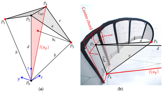
Figure 3.
Triangular two-plate model of the V3 kite. (a) Geometric definitions. In blue, the coordinate system is given. The two triangles shaded in grey represent the wing, point is the bridle point, and the triangle shaded in red lies in the symmetry plane. Adapted from [29]. (b) Definition of the points , and , defining the triangular plate representing one half wing. Photo taken from the ground in July 2012.
As seen in Figure 1a and Figure 2a, the central front bridle lines split into two line segments to better distribute the transmitted force to the LE and strut tubes. The distance d is measured from the bridle point to the virtual attachment point, where the bridle line would intersect the chord without the Y split. Accordingly, the length is measured from this virtual attachment point to the TE, as illustrated in Figure 3b.
Representing the two half wings as rigid triangular plates implies that the edges with lengths a, and e remain constant at the values specified in Table 3. The rigid plates are connected by four idealised bridle lines of lengths b, d and , with two for supporting the centre chord at points and and two for supporting each wing tip at points and . To formulate an analytical model, all bridle lines are assumed to be straight and attached directly to point . The bridle lines connecting to the centre of the LE and the two wing tips are assumed to be of constant length. Only the length of the central rear bridle line is assumed to be variable and a function of the power setting . Points and are assumed to be fixed to provide a reference to calculate the shape changes from [29].
Table 3.
Lengths derived from the designed (CAD) geometry of the TU Delft V3 kite in a fully powered state.
Using Equation (2), the length of the central rear bridle line can be related to the power setting
where represents the minimal length when powered. The division of by two is an approximation introduced by Oehler and Schmehl [5] to account for the pulleys in the bridle lines attached to the TE. Because the pulleys are at an angle to the central rear bridle line, the diagonal pulley extension is converted to a vertical central rear bridle line extension by adding a term.
2.3.1. Tetrahedon Algorithm
As illustrated in Figure 3, the points and as well as and span two mirrored irregular tetrahedra. The wing width w is defined as the geometric distance between the LE tip attachment points and of the bridle lines. Because of the symmetry plane spanned by points , and , one can calculate the width using the tetrahedron height (see Figure 3), defined as the perpendicular distance of each wing tip from the symmetry plane
The height can be calculated from the tetrahedron base area and the tetrahedron volume as follows
The volume is computed from the edge lengths as follows [37]
where the coefficients and are defined as
Using Heron’s formula for calculating the area of a triangle with sides A, B and C, we have
The tetrahedron’s base area can be calculated as follows
2.3.2. Trilateration Algorithm
With a trilateration algorithm that solves the intersection problem of three spheres [38], one can analytically calculate the coordinate changes instead of only the width change. This problem generally has two intersection points but is best visualised in 2D, where only one intersection point is shown, as illustrated in Figure 4a.
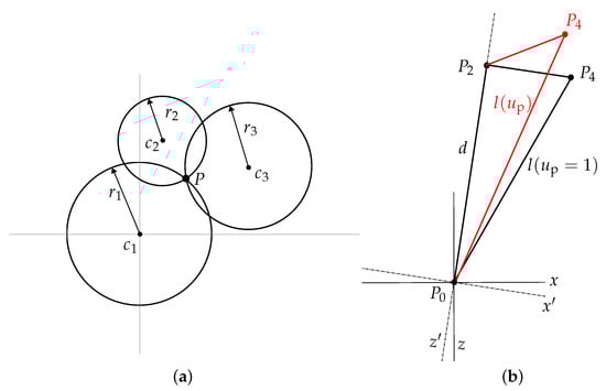
Figure 4.
Trilateration algorithm. (a) A 2D illustration of the intersection point P of three spheres, with sphere centres and and sphere radii , and , respectively [29]. (b) Illustration to support the calculations of the new location of . In black the powered shape ( = 1) is shown and in red a depowered state. Note that the depicted shape in black does not correspond to the design geometry but to the pre-simulated shape.
To calculate the deformation of the triangular two-plate model geometry, the locations of points , and must be determined. Because remains in the symmetry plane, one can determine its new location by solving the intersection problem of two circles. The circles have centres and and radii d and . An axis rotation is introduced as () to make both circle centres fall on the same axis (see Figure 4b). Using the rotated axis, the circle equations become
By rewriting and substituting the circle equations, one finds the location of in the rotated axis system
Using the principle of similar triangles, the location of can be found in the original axis () using
where the entry is equal to zero due to the present symmetry plane (see Figure 3a).
With the location of point and the points and as sphere centres with the lines and e as sphere radii, the coordinates of point and are defined as
where and are defined as
The tetrahedron and trilateration algorithms provide geometric constraint-based analytical solutions for the wing width and height as functions of the power setting. The trilateration algorithm requires three known points in space with three known distances to the desired point. Therefore, straight lines of constant lengths are assumed. The tetrahedron algorithm requires straight lines of known lengths. These assumptions limit the applicability of the analytical model because some bridle line systems, such as the bridle line system of the V3 kite, also include quadrilateral and pentagon line layouts (see Figure 1b) which, unlike purely triangular layouts, are not geometrically defined by the line lengths only [29].
2.4. Multi-Segment Wing Model
To include spanwise bending and torsion of the wing, slacking bridle lines, asymmetric control input and canopy billowing, the geometric modelling concept introduced in Section 2.3 is expanded into a force-based concept. This concept is based on the observation that the bridle line system transfers most of the load and dominates the shape of the kite. A particle system model (PSM) approach was chosen for its capacity to deal with bridle lines [23,39] and its low computational cost compared with other structural models (e.g., finite-element models) [40].
Because of the low mass of the membrane wing, the time scale of inertial effects is substantially lower than the time scales of flight manoeuvres and associated deformation phenomena. Consequently, it can be assumed that the kite transitions through a sequence of quasi-steady flight and deformation states while advancing along the flight trajectory [10,41]. Dynamic effects can be neglected, and consequently, a quasi-steady PSM is developed. Bosch et al. [22] used a quasi-steady PSM to represent the tether and bridle lines and couple this model to an FSI model of the wing to simulate the kite deformation while flying crosswind manoeuvres. Our approach differs, as non-physical compliance elements are not needed for stability. The same modelling technique represents the bridle line system and the wing by using point masses and connecting these with force-based distance constraints. The integrated bridle line system and wing model can describe both aero-structural and actuation-induced deformation phenomena.
As a force-based model, the PSM alleviates the assumption of straight and constant-length bridle lines such that the bridle line system of the V3 kite can be simulated. To simplify the problem, the chordwise Y splits of the bridle lines close to the LE are neglected, and two bridle line attachment points are relocated from between the struts to the outermost struts. The layout of the bridle line system and the lengths of the individual line segments are detailed in Appendix A. As illustrated in Figure 5a, the bridle lines are represented as massless spring-damper elements, and the bridle-line connection points are represented as particles.
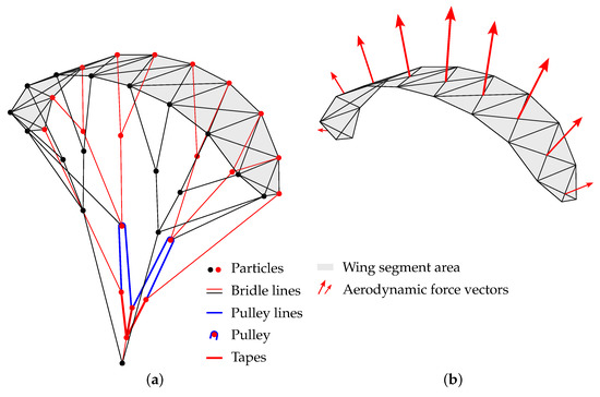
Figure 5.
Aero-structural model of the TU Delft V3 kite, adapted from [29]. (a) Structural model using a particle system approach, where each line represents a spring-damper element, and each dot represents a point mass. The two diagonal lines per wing segment are additional spring-damper elements used as cross members to prevent shear deformation. (b) Aerodynamic model of the segmented wing, with red arrows indicating the wing element’s aerodynamic force vectors.
The wing is discretised into spanwise segments, where each segment is defined between the struts, except for the outermost segments. Assuming that the bridle lines make up all the inter-wing segment rotational deformation resistance, the segments can be modelled as free to rotate over the struts. The edge of each segment is represented by a spring-damper element, and as the wing is mainly made of elongation-resisting fabric, all these elements have an elongation-resisting spring. A compression-resisting spring-damper element is added for the elements representing the tubular frame. In practice, this is equal to assuming that the tubular frame is of a constant length for the observed loads and used stiffness value. The TE spring-damper element has no compression-resisting spring stiffness, representing canopy billowing. Furthermore, diagonal elements are added to each segment to represent the membrane’s elongation-resisting properties which prevent shear deformation.
2.4.1. Equations of Motion
To find the displacements of the particles, the PSM solves for the force equilibrium for each particle
where is the aerodynamic force detailed in Section 2.4.2, is the structural force detailed in Section 2.4.3 and is the gravitational force, which is described as follows
where g is the gravitational constant. Together, a differential equation is formed, which is solved numerically as detailed in Section 2.4.4.
2.4.2. Aerodynamic Force
With Mach numbers well below 0.3, the flow around the kite can be assumed to be incompressible [29]. Furthermore, an inviscid flow is assumed, and 3D effects are neglected. The aerodynamic forces acting on the wing segments are assumed to be perpendicular to the segments. Only the induced drag is modelled, as viscosity is neglected. The resultant aerodynamic force generated by the wing can be assembled as the sum of all aerodynamic forces
The aerodynamic force of each segment is calculated using the lift equation
where represents the air density, is the apparent wind speed, is the projected wing segment surface area and is the lift coefficient. Following thin airfoil theory [42], a linear lift-polar is assumed, and the lift coefficient is found using
The angle of attack is defined as the angle between the apparent wind velocity and the centre chord line of each wing segment. Because the wing segments differ in size and angle with respect to the incoming wind, the wing segment aerodynamic force vector magnitudes and orientations differ, as illustrated in Figure 5b.
For coupling the aerodynamic model to the structural model, 75 percent of the wing segment’s aerodynamic force is applied to the front corner points, and 25 percent is applied to the rear corner points. An uneven distribution is chosen to include the chordwise loading differences present on an LEI airfoil under nominal operating conditions [43].
2.4.3. Structural Spring-Damper Elements
All mass is lumped at the particles, forming connections between the massless elements, and modelled as frictionless hinges. The structural force (i.e., linear damping force and linear spring force on each particle ), as a result of the connected elements is determined using
where represents the damping coefficient, is the number of connected elements, is the unit vector pointing along the element and represents the element stiffness. The damping force scales with the particle’s velocity and acceleration and the spring force of each element with the elongation.
When describing the location of two connected particles (), the non-dimensional element elongation becomes
where is the current length and is the rest length of the element [39].
Ideal pulleys are assumed to be frictionless, which means that the pulley line’s tensile force must be equal on both sides of the pulley. A schematic of a pulley is present in Figure 6, where the pulley line runs from knot over a pulley and to another knot . The tensile force in the described pulley line can be calculated from Equation (38) using an adjusted elongation term
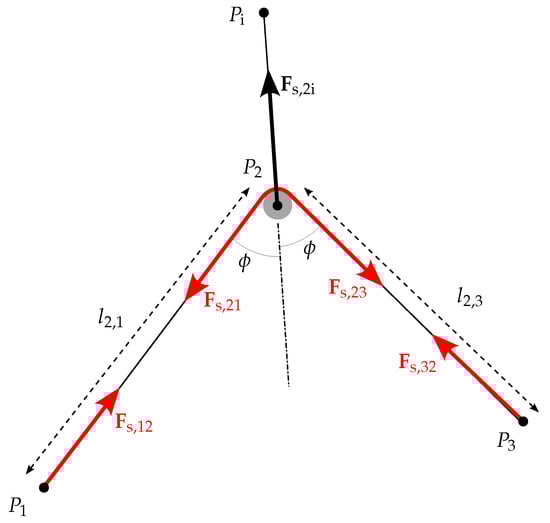
Figure 6.
Force equilibrium at a pulley connected via bridle line to knot . The bridle line that runs over the pulley connects knots and , the corresponding tensile spring force is shown in red. For an ideal, frictionless pulley, the line angles are identical [29].
2.4.4. Numerical Solver
The PSM equations of motion form a system of second-order, non-homogeneous ordinary differential equations
where represents the mass matrix filled with masses and is the position vector of all the particles. The differential equations are solved iteratively using the process illustrated in Figure 7. The problem is loosely coupled (i.e., the structural and aerodynamic models iterate until convergence before they interact). The loosely coupled iterations are solved using a Runge–Kutta method of the fifth order [44], implemented using the initial value problem solver scipy package of Python. This implicit method is chosen over an explicit method because the differential equations are stiff.
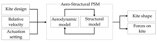
Figure 7.
Flowchart of the aero-structural PSM.
2.4.5. Static Equilibrium
To find a static equilibrium at which the simulation can converge, an equilibrium must hold over the three translational and three rotational degrees of freedom. In an AWE system, the bridle point attaches the kite to the tether. This is modelled as a boundary condition by a ball joint constraint at the bridle point. The ball joint constraint induces an equal and opposite force, which in a full system would be the tether force, therefore providing an equilibrium over the translational degrees of freedom. The ball joint constraint, similar to the bridle point in an AWE system, does not restrict any rotation.
In idealised conditions with zero steering input, the kite has the same symmetry plane as the triangular two-plate model (see Figure 3a). As a result of the symmetry, the force in the y direction, the yaw rotation over the z axis and the roll rotation over the x axis are all balanced by definition. This reduces the problem to one rotational and two translational degrees of freedom. The translational degrees of freedom find equilibrium due to the ball joint constraint. In a steady case, the remaining rotational degree of freedom over the y axis is balanced by gravity, the wing’s aerodynamic force and the spring force.
2.5. Photogrammetry
The kite geometry is subject to various changes induced by strong aero-structural coupling and actuation-induced wing morphing, which means that one should validate the form. The only available and useful data are from video footage, taken on the 24th and 30th of March 2017 by a camera attached to the KCU and pointing towards the wing [29]. Extracting information from photogrammetric data is possible in multiple ways, and examples are illustrated in Figure 8. The left figure shows how the pulleys move positions and how the TE wing tip folds outwards when powered. The right figure illustrates how the angle between the centre chord and the front lines increases when depowering (i.e., this is how the angle of attack is reduced).
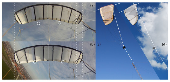
Figure 8.
TU Delft V3 kite in flight [5]. Wing planforms of the (a) depowered kite and the (b) powered kite were captured as video stills from recordings taken by the KCU onboard camera. Complete video is available from [34]. Side views of the (c) partially depowered kite during a landing manoeuvre and the (d) fully powered kite during a crosswind flight manoeuvre are shown with manual control from the ground, captured as photos taken by an observer on the ground.
For studying the deformations of the kite, the wing’s tip-to-tip width is chosen as an indicator because of its relation to the anhedral angle that affects many parameters (e.g., the aerodynamic load). Aside from the width, the trailing edge strut’s tip-to-tip length change is also measured, indicating the canopy billowing. Ideally, one would extract the lengths as a function of time and the control setting. However, this is infeasible, as only visual and audio information is available for the filmed flights. There are other measurements available from different flights on the 24th of March [36], but unfortunately, they are not of the same flight. The video footage is therefore reduced to video stills which represent the extreme states, as these are most identifiable and useful for validation. For straight flight, multiple video stills were collected of the kite in its powered state during reel out as well as multiple stills in its depowered state during reel in. For turning flight, it was concluded that the footage was too distorted to be used quantitatively [29].
To extract measurements from the video stills, post-processing is required. The optical distortion induced by the camera’s fish eye lens is removed by using an opposite lens filter whose magnitude is tuned such that the curved horizon present in several images appears straight again [29]. The camera covers a specific physical area (i.e., a rectangle on a wall for a projector), whose size depends on its focal length, lens, aperture and the distance between the camera lens and the object. This area can be divided by the pixel resolution to find a meter-to-pixel ratio, which is needed to convert the tip-to-tip pixel width to meters. The camera’s focal length, lens and aperture were constant during the measurement campaign, but the distance varied. The distance variations were caused by swinging of the KCU with the attached camera, wing pitching and wing deformation. Due to these variations, the exact projection distance at each video is unknown.
Therefore, instead of defining the meter-to-pixel ratio using the distance to the object, the differences are expressed in percentages and converted to meters using the dimensions of the design geometry. The design geometry is used as it was known upfront. To obtain the meter-to-tip ratios used for the TE tip-to-tip distance conversions, the struts are assumed to remain at a constant length. By defining the ratios locally, the distortion caused by the wing’s non-perpendicularity is taken into account.
3. Results
The described photogrammetry analysis showed, on average, a 5% decrease in width between the powered and depowered states, with a standard deviation of approximately 3%. As this is the first quantitative measurement effort into the form changes in the V3, the results can only be compared to qualitative observations, which confirm the decrease in width when powered [5]. The trailing edge strut tip-to-tip lengths, indicating billowing, increased the width on average by 2.4 percent when changing from powered to the depowered state [29]. When including billowing, the diagonal elements restricted the movement and were therefore increased by five percent to represent the initial absent stretch resistance of the canopy. It should be noted that the photogrammetry results were most accurate in the proportional change and less accurate in the magnitude. The width results were specifically scaled based on the design geometry, which was qualitatively observed to differ from the powered state (see Figure 2b).
The rest of this section presents a comparison between the photogrammetry and simulation results for the two wing models using values of both 8 percent and 13 percent and for the multi-segment wing model with and without billowing as well.
3.1. Triangular Two-Plate Wing Model
Two novel models were developed for the two-plate wing model, and both are pure geometric constraint-based analytical models. Because the design was made without knowing the form deformations due to the aero-structural coupling, and the two-plate model is a simplified representation of the wing geometry, a pre-simulation was performed using the PSM method, which was applied to the two-plate triangular model. In the design state, which represents the powered state, where , the design geometry and pre-simulation showed different values. The pre-simulated wing geometry was flatter, which made the width value higher. The lengths of the design geometry and those derived from the pre-simulation of the kite are listed in Table 3. Furthermore, to find , the angle is needed (see Equation (6)), which is assumed to remain equal to 27 and is derived from the design geometry.
The tetrahedron and trilateration algorithms were used to simulate the design geometry with a value of 8 percent and the pre-simulated geometry using values of 8 percent and 13 percent. The results are plotted together with the photogrammetry measurements in Figure 9a.
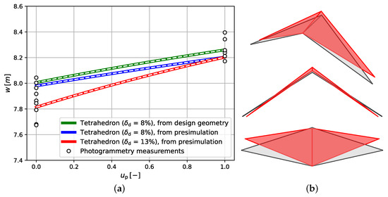
Figure 9.
Triangular two-plate results. (a) Wing width determined by photogrammetry and the triangular two-plate model results, calculated as a function of the power setting () using a tetrahedron algorithm. The trilateration algorithm results serve as verification and are indicated by the white dashed lines. (b) Form deformation of the triangular two-plate model, showing the design geometry in grey and the depowered state () in red, calculated with the trilateration algorithm. From top to bottom, isometric, front and top views of the triangular two-plate model are displayed.
The width predictions of the tetrahedron and trilateration algorithms overlap perfectly, thereby verifying the two models (see Figure 9a). The analytical width predictions showed a nonlinear increase from depowered to the powered state. The increase in width, also shown by the photogrammetry measurements, was as expected because when increasing the wing loading, the wing should flatten. Compared with the photogrammetry measurements, the powered state width predictions that started from the design geometry were, as they should be, at the mean of the photogrammetry. This was not the case for the simulations starting from the simulated shape. At = 0, the results using = 13% seemed to overpredict the width, whereas those using 8 percent seemed to underpredict the width. All simulation results at both the powered and depowered states were within the range of photogrammetric measurements and thus seemed to agree well.
3.2. Multi-Segment Wing Model
To run the force-based PSM, several values had to be set. A trial-and-error procedure was used to determine the absolute error, relative error, maximum step size and simulation time interval (see Table 4).
Table 4.
Parameters and computational settings [29].
Because a static kite under idealised conditions was modelled, the apparent wind speed used to determine the aerodynamic force (see Equation (34)) was equal to the set wind speed (see Table 4).
As the interest was only in the steady state solution, the parameters that affected only the transient phase could be set at non-physical values as long as they did not affect the steady state solution. The parameters affecting only the transient phase were those involving velocity or acceleration (i.e., the damping and inertial forces). For a single-mass spring-damper system, one can determine the critical damping coefficient, but for a particle system model with more than two particles, there is not one critical damping coefficient. Therefore, the damping constant was assumed to be equal for all elements and determined by trial and error. It was initially equal to the value present in Table 4 and increased over the simulation time interval to a value of one to dampen out all remaining vibrations.
Furthermore, the mass matrix was filled with the same mass value . In part because the inertial forces do not affect the steady state solution, the value m (see Table 4) was determined by equally distributing the total kite mass of kg (see Table 1b) over the particles (37 here). The gravitational force did affect the steady state solution and thus required the proper mass distribution. The effect was assumed to be negligible and left for future work, where other efforts into mass distribution should be considered [20,45].
Over each time step, the spring force was assumed to remain constant, which caused stability problems when using the physical stiffness values. To solve the problem within a reasonable time frame, a limitation was set on the minimal time step size. To converge, each element was assumed to have the same lower-than-physical stiffness value (see Table 4). The global stiffness value K was selected by trial and error, and thus the maximum bridle line elongation in a steady state was below 3 percent.
The force-based PSM was applied to the multi-segment representation of the V3 kite wing using values of both 8 percent and 13 percent with and without TE canopy billowing (see Figure 10). The PSM matched the photogrammetry results well with values of both 8 percent and 13 percent. Compared with the constraint-based analytical tetrahedon results, the PSM with a value of 8 percent predicted a less steep decrease in width.
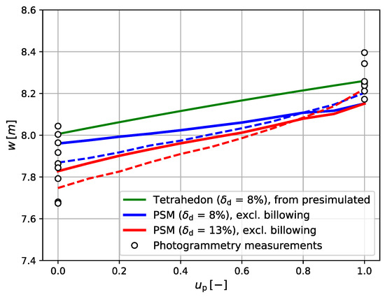
Figure 10.
Photogrammetry results plotted together with the PSM results and a two-plate model tetrahedron result as a function of the power setting (). The dashed lines depict the simulation which includes billowing, with blue for a value of 8% and red for 13%.
Including billowing (i.e., increasing the rest lengths of the TE and diagonal elements) decreased the width predicted in the powered state but increased in the depowered state. In other words, the effect of including billowing was that the width changed less as a result of increasing the rear bridle lines’ lengths through a depower tape extension.
When comparing the form changes shown in Figure 11, one can observe that the powered shape showed the expected pitching compared with the design geometry (i.e., it fell backwards in the direction of the wind, where it found equilibrium between the aerodynamic force, spring force and gravity). Furthermore, the LE tips seemed to fold outwards, and the TE tip seemed to fold inwards. This is precisely the same as what was qualitatively observed in Figure 8. The overlap between the simulations and qualitative photogrammetric comparison illustrates the importance of considering the differences between the powered shape and the design geometry.
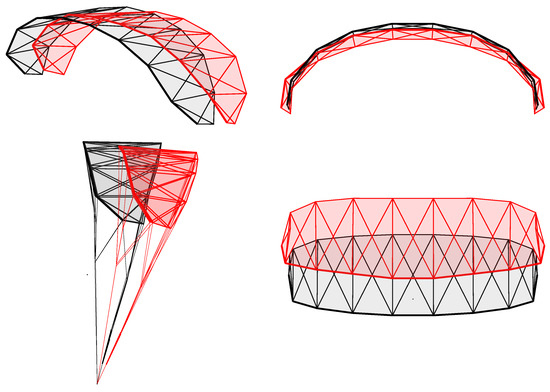
Figure 11.
Shape deformation resulting from symmetric actuation of the rear bridle line system in a fully powered state ( = 1), with = 13% and including billowing. The grey-graded shape corresponds to the design geometry, and the red shape represents the powered state. From top to bottom and left to right, an isometric view, a front view, a side view and a top view are displayed. The thicker edge line panel indicates the front of the panel but does not correspond to the LE tube. The side view results are symmetrical but do not appear so due to the viewing position misalignment with the wing.
When comparing the powered and depowered shapes (see Figure 12), the depowered kite pitched further backwards. Measured from the horizontal bridle point plane, the angle of the powered front bridle lines was 86 , and when depowered, it was 75 . This is attributed to the depowered state generating less lift and more drag. With less lift, the gravity and drag proportional contributions increased, which caused increased pitching. In the simulations, less lift was generated in the depowered state due to the inward fold of the TE tips and increased the anhedral angle.
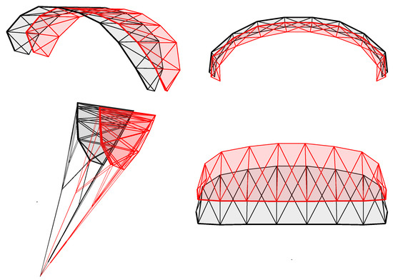
Figure 12.
Shape deformation resulting from symmetric actuation of the rear bridle line system in a fully depowered state ( = 0), with = 13% and including billowing. The grey graded shape corresponds to the powered shape with = 1, and the red shape represents the depowered state. From top to bottom and left to right, an isometric view, a front view, a side view and a top view are displayed.
By introducing a non-physical boundary condition, one can converge asymmetrical deformation (e.g., due to nonzero steering input). The new boundary condition is a point that has spring-damper elements attached to the front particles of the middle panel, thereby restricting them from moving away. The new point is placed in between the two particles, and the elements have a stiffness of 2 × 10³ N /m. In this way, the yaw and roll rotational degrees of freedom are constrained, enabling the solution of an asymmetric input. Using a steering input of , a left turn is illustrated in Figure 13. Even though the boundary condition was non-physical, the results did qualitatively match the photogrammetric data because the expected twist and inward bending of the tips were shown [5].
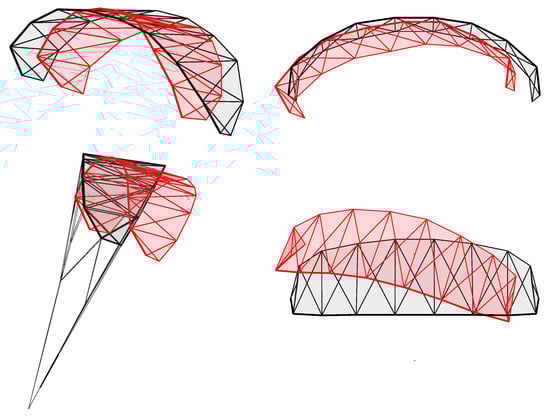
Figure 13.
Shape deformation resulting from symmetric actuation of the rear bridle line system with = 0.12, = 1 and = 13%. The grey graded shape corresponds to the powered shape with = 1, and the red shape corresponds to the asymmetrical deformed state. From top to bottom and left to right, an isometric view, a front view, a side view and a top view are displayed.
4. Conclusions and Discussion
This paper presented two novel structural models for airborne soft wing kites that harvest wind energy. Modelling the deformations is necessary, as it uses a morphing wing control surface and is subject to strong aero-structural coupling.
Photogrammetry analysis was conducted of video footage from a camera strapped to the airborne kite control pod hanging beneath the kite. On average, the span differed by 5 percent when comparing the powered and depowered states. The trailing edge strut’s tip-to-tip canopy length measurements, indicating billowing and used as empirical relations, showed an average increase of 2.4 percent when comparing the powered and depowered states. The uncertainty was deemed too high for quantitative analysis of turning flight.
The modelling approach assumes that the bridle line system’s geometry primarily influences the global geometry of the aerodynamically loaded membrane wing. The geometric distances between the wing-attached bridle line points were assumed to remain constant due to the compressive and tensile stiffness of the inflated tubular frame. The TU Delft V3 kite of 25 m2 was used, which was fully supported by front and rear bridle line systems. The kite was controlled through adjustments of the steering and depower tapes, for which dimensionless parameters were introduced to represent the power and steering settings. The flight data, taken during different flights than the footage, showed both an 8 percent and 13 percent deployed depower tape of the maximum deployable length.
A triangular two-plate model was developed to predict the actuation-induced symmetric deformation analytically. Each wing half was modelled as a rigid triangular plate. Therefore, deformation phenomena such as billowing or span-wise bending were neglected. Four idealised bridle lines attached the plate’s corner points to the bridle line point. A relation between the length of the rear bridle line and the power setting was developed. A novel tetrahedron algorithm using geometric tetrahedron relations and a trilateration algorithm that solves the intersection problem of three spheres were developed. Both showed identical results and predicted a nonlinear decrease in width when depowering, aligning with the photogrammetry analysis.
The triangular two-plate model is a pure geometric constraint-based analytical model requiring geometrically determined shapes. For more complex shapes (e.g., the pentagons present in the bridle line system), a force-based method is needed. A multi-segment wing model is defined using a particle system model, where each segment consists of four point masses kept at a constant distance along the tubular frame by linear spring-damper elements. The same massless elements also represent the line segments of the bridle line system, with each connecting two point masses. The particle system model incorporates aerodynamic forces on each wing segment and represents both the steering and depower tape, hence allowing for the prediction of symmetric and asymmetric deformations resulting from bridle line actuation. With the current set-up, an additional boundary condition was required to converge the asymmetrical case.
Future work should validate the predicted shape changes with more parameters than the width. A finer wing discretisation could be used (e.g., including the bridle line forking near the leading edge). Several aerodynamic model assumptions are unnecessary when using the work of Cayon [30]. Developing billowing relations instead of using empirical data would make the model calibration independent. Lastly, a solution that enables the model to deal with asymmetries without non-physical constraints must be found.
Author Contributions
Conceptualisation, J.A.W.P. and R.S.; methodology, J.A.W.P.; software, J.A.W.P.; validation, J.A.W.P.; formal analysis, J.A.W.P.; resources, J.A.W.P. and R.S.; writing—original draft preparation, J.A.W.P.; writing—review and editing, J.A.W.P. and R.S.; visualisation, J.A.W.P.; supervision, R.S. All authors have read and agreed to the published version of the manuscript.
Funding
This work is part of the NEON research program and received funding from the Dutch Research Council NWO under Grant Agreement No. 17628 and co-funding from Kitepower B.V. The APC was covered by Delft University of Technology.
Data Availability Statement
A Python implementation of the triangular two-plate model described in this paper is available from the repository at https://github.com/awegroup/TUD-V3-kite-depower-2plate (accessed on 12 May 2023).
Acknowledgments
The authors would like to thank the staff of Kitepower B.V. for answering questions and providing video footage of test flights.
Conflicts of Interest
Both authors are full-time employees of Delft University of Technology. R.S. is a co-founder of Kitepower B.V., which provided the video footage of the test flights and some additional information about the hardware set-up.
Abbreviations
The following abbreviations are used in this manuscript:
| AWE | Airborne wind energy |
| CAD | Computer-aided design |
| CFD | Computational fluid dynamics |
| FE | Finite element |
| FSI | Fluid–structure interaction |
| GPS | Global positioning system |
| IMU | Inertial measurement unit |
| KCU | Kite control unit |
| LE | Leading edge |
| PSM | Particle system model |
| TE | Trailing edge |
Appendix A. Multi-Segment Wing Model Bridle Plan
Figure A1 details the bridle plan employed for the multi-segment wing model of the TU Delft V3 kite operated by Kitepower B.V. in March 2017. The planform shows the flat, unrolled wing. The steering tape is in the neutral position, and the depower tape is in the powered position. The indicated lengths of the bridle lines are given in millimetres. A typical diameter for the bridle lines is 2.5 mm. As described in Section 2.4, the chordwise Y splits of the bridle lines close to the LE were not taken into account in the simulation model. Accordingly, the bridle lines attach at the projected points LE1–LE4.

Figure A1.
Bridle plan used during the simulations. The left side indicates bridle lines attached at the TE, and the right side indicates those attached at the LE. The dots a1, b1, c1, d1, a2, etc. represent possible bridle line attachment points.
Figure A1.
Bridle plan used during the simulations. The left side indicates bridle lines attached at the TE, and the right side indicates those attached at the LE. The dots a1, b1, c1, d1, a2, etc. represent possible bridle line attachment points.

References
- Watson, S.; Moro, A.; Reis, V.; Baniotopoulos, C.; Barth, S.; Bartoli, G.; Bauer, F.; Boelman, E.; Bosse, D.; Cherubini, A.; et al. Future emerging technologies in the wind power sector: A European perspective. Renew. Sustain. Energy Rev. 2019, 113, 109–270. [Google Scholar] [CrossRef]
- Van Hagen, L.; Petrick, K.; Wilhelm, S.; Schmehl, R. Life-Cycle Assessment of a Multi-Megawatt Airborne Wind Energy System. Energies 2023, 16, 1750. [Google Scholar] [CrossRef]
- Bechtle, P.; Schelbergen, M.; Schmehl, R.; Zillmann, U.; Watson, S. Airborne wind energy resource analysis. Renew. Energy 2019, 141, 1103–1116. [Google Scholar] [CrossRef]
- Kleidon, A. Physical limits of wind energy within the atmosphere and its use as renewable energy: From the theoretical basis to practical implications. Meteorol. Z. 2021, 30, 203–225. [Google Scholar] [CrossRef]
- Oehler, J.; Schmehl, R. Aerodynamic characterization of a soft kite by in situ flow measurement. Wind Energy Sci. 2019, 4, 1–21. [Google Scholar] [CrossRef]
- Kitepower Airborne Wind Energy-Plug & Play, Mobile Wind Energy. Available online: https://thekitepower.com/ (accessed on 12 July 2022).
- Van den Heuvel, J. Kitesailing: Improving System Performance and Safety. Master’s Thesis, Delft University of Technology, Delft, The Netherlands, 2010. Available online: http://resolver.tudelft.nl/uuid:cee4dcf5-e2a8-49d0-b731-92db25b44a17 (accessed on 1 October 2021).
- Oehler, J.; van Reijen, M.; Schmehl, R. Experimental Investigation of Soft Kite Performance During Turning Maneuvers. J. Physics: Conf. Ser. 2018, 1037, 052004. [Google Scholar] [CrossRef]
- Breukels, J. An Engineering Methodology for Kite Design. Ph.D. Thesis, Delft University of Technology, Delft, The Netherlands, 2011. Available online: http://resolver.tudelft.nl/uuid:cdece38a-1f13-47cc-b277-ed64fdda7cdf (accessed on 1 July 2023).
- Roullier, A. Experimental Analysis of a Kite System’s Dynamics. Master’s Thesis, EPFL, Lausanne, Switzerland, 2020. [Google Scholar] [CrossRef]
- Baayen, J.; Ockels, W. Tracking control with adaption of kites. IET Control Theory Appl. 2011, 4, 182–191. [Google Scholar] [CrossRef]
- Van der Vlugt, R.; Bley, A.; Noom, M.; Schmehl, R. Quasi-steady model of a pumping kite power system. Renew. Energy 2019, 131, 83–99. [Google Scholar] [CrossRef]
- De Groot, S.G.C.; Breukels, J.; Schmehl, R.; Ockels, W.J. Modeling Kite Flight Dynamics Using a Multibody Reduction Approach. J. Guid. Control. Dyn. 2011, 34, 1671–1682. [Google Scholar] [CrossRef]
- Jehle, C.; Schmehl, R. Applied Tracking Control for Kite Power Systems. J. Guid. Control. Dyn. 2014, 37, 1211–1222. [Google Scholar] [CrossRef]
- Schelbergen, M.; Schmehl, R. Validation of the quasi-steady performance model for pumping airborne wind energy systems. J. Phys. Conf. Ser. 2020, 1618, 032003. [Google Scholar] [CrossRef]
- Vermillion, C.; Cobb, M.; Fagiano, L.; Leuthold, R.; Diehl, M.; Smith, R.S.; Wood, T.A.; Rapp, S.; Schmehl, R.; Olinger, D.; et al. Electricity in the Air: Insights From Two Decades of Advanced Control Research and Experimental Flight Testing of Airborne Wind Energy Systems. Annu. Rev. Control 2021, 52, 330–357. [Google Scholar] [CrossRef]
- Gohl, F.; Luchsinger, R.H. Simulation Based Wing Design for Kite Power. In Airborne Wind Energy; Ahrens, U., Diehl, M., Schmehl, R., Eds.; Green Energy and Technology; Springer: Berlin/Heidelberg, Germany, 2013; Chapter 18; pp. 325–338. [Google Scholar] [CrossRef]
- Erhard, M.; Strauch, H. Control of Towing Kites for Seagoing Vessels. IEEE Trans. Control. Syst. Technol. 2013, 21, 1629–1640. [Google Scholar] [CrossRef]
- Fagiano, L.; Zgraggen, A.; Morari, M.; Khammash, M. Automatic crosswind flight of tethered wings for airborne wind energy: Modeling, control design and experimental results. IEEE Trans. Control. Syst. Technol. 2014, 22, 1433–1447. [Google Scholar] [CrossRef]
- Fechner, U.; Van der Vlugt, R.; Schreuder, E.; Schmehl, R. Dynamic Model of a Pumping Kite Power System. Renew. Energy 2015, 83, 705–716. [Google Scholar] [CrossRef]
- Breukels, J.; Schmehl, R.; Ockels, W. Aeroelastic Simulation of Flexible Membrane Wings based on Multibody System Dynamics. In Airborne Wind Energy; Ahrens, U., Diehl, M., Schmehl, R., Eds.; Green Energy and Technology; Springer: Berlin/Heidelberg, Germany, 2013; Chapter 16; pp. 287–305. [Google Scholar] [CrossRef]
- Bosch, A.; Schmehl, R.; Tiso, P.; Rixen, D. Dynamic nonlinear aeroelastic model of a kite for power generation. J. Guid. Control. Dyn. 2014, 37, 1426–1436. [Google Scholar] [CrossRef]
- Geschiere, N. Dynamic Modelling of a Flexible Kite for Power Generation: Coupling a Fluid-Structure Solver to a Dynamic Particle System. Master’s Thesis, Delft University of Technology, Delft, The Netherlands, 2014. Available online: http://resolver.tudelft.nl/uuid:6478003a-3c77-40ce-862e-24579dcd1eab (accessed on 18 May 2021).
- Leloup, R.; Roncin, K.; Bles, G.; Leroux, J.B.; Jochum, C.; Parlier, Y. Estimation of the lift-to-drag ratio using the lifting line method: Application to a leading edge inflatable kite. In Airborne Wind Energy; Ahrens, U., Schmehl, R., Diehl, M., Eds.; Springer: Berlin/Heidelberg, Germany, 2013; Chapter 19; pp. 339–355. [Google Scholar] [CrossRef]
- Drela, M. XFOIL Subsonic Airfoil Development. Available online: https://web.mit.edu/drela/Public/web/xfoil/ (accessed on 18 May 2021).
- De Solminihac, A.; Alain Nême, C.D.; Leroux, J.B.; Roncin, K.; Jochum, C.; Parlier, Y. Kite as a Beam: A fast Method to get the Flying Shape. In Airborne Wind Energy—Advances in Technology Development and Research; Schmehl, R., Ed.; Green Energy and Technology; Springer: Singapore, 2018; Chapter 4; pp. 79–97. [Google Scholar] [CrossRef]
- Duport, C. Modeling with Consideration of the Fluid-Structure Interaction of the Behavior under Load of a Kite for Auxiliary TRACTION of Ships. Ph.D. Thesis, University of Bretagne, Brest, France, 2018. Available online: https://theses.hal.science/tel-02383312 (accessed on 1 September 2022).
- Van Til, J.; De Lellis, M.; Saraiva, R.; Trofino, A. Dynamic model of a C-shaped bridled kite using a few rigid plates. In Airborne Wind Energy—Advances in Technology Development and Research; Schmehl, R., Ed.; Green Energy and Technology; Springer: Singapore, 2018; Chapter 5; pp. 99–115. [Google Scholar] [CrossRef]
- Poland, J.A.W. Modelling Aeroelastic Deformation of Soft Wing Membrane Kites. Master’s Thesis, Delft University of Technology, Delft, The Netherlands, 2022. Available online: http://resolver.tudelft.nl/uuid:39d67249-53c9-47b4-84c0-ddac948413a5 (accessed on 1 April 2023).
- Cayon, O. Fast Aeroelastic Model of a Leading-Edge Inflatable Kite. Master’s Thesis, Delft University of Technology, Delft, The Netherlands, 2022. Available online: http://resolver.tudelft.nl/uuid:aede2a25-4776-473a-8a75-fb6b17b1a690 (accessed on 1 June 2023).
- Coenen, R. Single Skin Kite Airfoil Optimization for Airborne Wind Energy Systems. Master’s Thesis, Delft University of Technology, Delft, The Netherlands, 2018. Available online: http://resolver.tudelft.nl/uuid:fdcf8423-11f0-4b33-956e-3e761635ac41 (accessed on 1 April 2023).
- Schmehl, R. Successful Mast-Based Launch of the V3 Kite; Delft University of Technology: Delft, The Netherlands, 2020. [Google Scholar] [CrossRef]
- Salma, V.; Friedl, F.; Schmehl, R. Improving Reliability and Safety of Airborne Wind Energy Systems. Wind Energy 2019, 23, 340–356. [Google Scholar] [CrossRef]
- Schmehl, R.; Oehler, J. 25 m2 LEI V3 Tube Kite Transitioning to Traction Phase, Flying Figure Eight Manoeuvres; Copernicus Publications: Göttingen, Germany, 2018. [Google Scholar] [CrossRef]
- Fechner, U. A Methodology for the Design of Kite-Power Control Systems. Ph.D. Thesis, Delft University of Technology, Delft, The Netherlands, 2016. [Google Scholar] [CrossRef]
- Oehler, J.; Schmehl, R.; Peschel, J.; Faggiani, P.; Buchholz, B. Kite Power Flight Data Acquired on 24 March 2017; Dataset, 4TU; Centre for Research Data, TU Delft Library: Delft, The Netherlands, 2018. [Google Scholar] [CrossRef]
- Richards, D.; Amos, M. Shape Optimization With Surface-Mapped CPPNs. IEEE Trans. Evol. Comput. 2017, 21, 391–407. [Google Scholar] [CrossRef]
- Fang, B. Trilateration and extension to global positioning system navigation. J. Guid. Control. Dyn. 1986, 9, 715–717. [Google Scholar] [CrossRef]
- Williams, P. Cable Modeling Approximations for Rapid Simulation. J. Guid. Control. Dyn. 2017, 40, 7. [Google Scholar] [CrossRef]
- Schwoll, J. Finite Element Analysis of Inflatable Structures Using Uniform Pressure. Master’s Thesis, Delft University of Technology, Delft, The Netherlands, 2012. Available online: http://resolver.tudelft.nl/uuid:f92da57f-55df-4109-9f8a-8c7c2b220c6a (accessed on 1 July 2021).
- Leuthold, R. Multiple-Wake Vortex Lattice Method for Membrane Wing Kites. Master’s Thesis, Delft University of Technology, Delft, The Netherlands, 2015. Available online: http://resolver.tudelft.nl/uuid:4c2f34c2-d465-491a-aa64-d991978fedf4 (accessed on 1 November 2021).
- Anderson, J.D. Fundamentals of Aerodynamics, 5th ed.; McGraw-Hill Inc.: New York, NY, USA, 2016; pp. 346–352. [Google Scholar]
- Folkersma, M.; Viré, A. Flow transition modeling on two-dimensional circular leading edge airfoils. Wind Energy 2019, 22, 908–921. [Google Scholar] [CrossRef] [PubMed]
- Hairer, E.; Wanner, G. Stiff differential equations solved by Radau methods. J. Comput. Appl. Math. 1998, 111, 93–111. [Google Scholar] [CrossRef]
- Karadayi, M.C. Particle System Modelling and Dynamic Simulation of a Tethered Rigid Wing Kite for Power Generation. Master’s Thesis, Delft University of Technology, Delft, The Netherlands, 2016. Available online: http://resolver.tudelft.nl/uuid:d6a2fcf8-7fce-4eb8-857b-209b9faac755 (accessed on 1 April 2023).


Disclaimer/Publisher’s Note: The statements, opinions and data contained in all publications are solely those of the individual author(s) and contributor(s) and not of MDPI and/or the editor(s). MDPI and/or the editor(s) disclaim responsibility for any injury to people or property resulting from any ideas, methods, instructions or products referred to in the content. |
© 2023 by the authors. Licensee MDPI, Basel, Switzerland. This article is an open access article distributed under the terms and conditions of the Creative Commons Attribution (CC BY) license (https://creativecommons.org/licenses/by/4.0/).