Abstract
This paper presents a systematic and comprehensive mathematical model for alkaline water electrolyzer cells, which can be used for simulation and analysis. The model accounts for factors such as gas evolution reactions, dissolution of gases in the electrolyte, bubble formation, and charge transport. It is based on a numerical two-phase model using the Euler-Euler approach, which has been validated against experimental data for various current densities. The study compares the impact of varying potassium hydroxide (KOH) concentration, separator porosity, and electrolyte flow rates on two-phase flow and bubble coverage. Therefore, the electrolyte in the cell consists of a solution of potassium hydroxide in water. The formation of gas bubbles at the electrodes decreases the electrolyte’s ionic conductivity. Additionally, the presence of these bubbles on the electrode surfaces reduces the available surface area for electrochemical reactions, leading to an increase in the overpotential at a given current density. Furthermore, this paper demonstrates how a neural network and ensembled tree model can predict hydrogen production rates in an alkaline water electrolysis process. The trained neural network accurately predicted the hydrogen production rates, indicating the potential of using neural networks for optimization and control of alkaline water electrolysis processes. The model has an average R-squared value of 0.98, indicating a good fit to the data. A new method of describing bubble transfer, “bubble diffusion,” is introduced to improve performance and reduce costs. The model is solved using COMSOL Multi physics 6.0. The machine learning models in this study were built, trained, and tested using MATLAB software R2020a.
Keywords:
alkaline water electrolysis; hydrogen; bubble dispersion; ANN; ensembled tree model; MATLAB; COMSOL 1. Introduction
Energy challenges are now divided into two categories. One is tied to the risk of fossil resource depletion, while the other concerns environmental. Today’s sources of fossil fuels are limited in quantity. Fuel cells generate water, energy, and heat by reacting hydrogen and oxygen in a redox reaction [1,2]. However, these traditional energy sources have negative side effects, such as greenhouse gas emissions from burning hydrocarbons and the generation of difficult-to-treat waste from nuclear power. As traditional energy supplies are depleted, it is critical to develop alternative energy sources that can be stored and transported such as hydrocarbons. In this sense, hydrogen is a significant contender, despite the fact that it is merely an energy transporter and not a main resource [3]. Energy storage is a fundamental challenge when integrating renewable energy sources into an electrical grid, due to their intermittent nature and the need for a steady power supply. Today, the two most common technologies for producing hydrogen in commercial applications are alkaline electrolysis and proton exchange membrane electrolysis. Alkaline water electrolysis has several advantages over proton exchange membrane water electrolysis, including durability, low cost, and technical maturity [4].
In recent years, technological advances have led to improvements in the efficiency of alkaline water electrolysis. The efficiency of the process can be affected by a number of factors, including activation losses at the electrodes, ohmic losses in the electrolyzer equipment, reductions in the electrochemically active surface, and transport resistance caused by bubbles [4,5]. To address this issue, some researchers have explored using an anion exchange membrane instead of a separator. Another solution is the use of zero-gap cell designs, which involves using two porous electrodes on each side of a hydroxide ion transporting separator that are pressed together, creating a gap of less than 0.5 mm. This technique has been shown to significantly reduce the electrolyte resistance between the electrodes [6,7]. During the process of AWE, hydrogen and oxygen are produced, leading to various flow patterns of two-phase electrolytes in AWE cells. Bubble production increases flow around the electrodes, which improves the transfer of electroactive substances. The performance of alkaline water electrolysis (AWE) technologies can be greatly impacted by the growth of bubbles.
Several studies have been conducted to investigate the behavior of bubbles and their effect on the performance of AWE cells. As a result, the influence of the bubble on efficiency must be accurately predicted or simulated. The first well-known study on this topic was conducted by Tobias et al. [8] and Hine et al. [9]. Both investigations concentrated on the influence of bubbles on electrolyte resistance. Studies in electrolysis make use of CFD models to understand bubble behavior. The models come in two types, Euler-Euler and Euler–Lagrange, with Euler-Euler having two categories: mixtures and two-phase fluids. Some studies have used the two-fluid model. These models provide information on bubble hydrodynamics, phase interactions, species transport, and gas hold-up [10]. Huang et al. focus on the synthesis and characterization of tensile-strained RuO2 loaded on antimony–tin oxide (ATO) using a fast quenching technique for proton-exchange membrane water electrolyzers [11]. Guan et al. present a groundbreaking study on the role of strain and reconstruction effects in catalytic reactions [12]. Eigeldinger and Vogt [13] conducted extensive experiments and theoretical analyses to examine the impact of electrolyte velocity on bubble movement in electrochemical systems. Their research showed that the velocity of the electrolyte is a crucial factor in determining the transport of bubbles. These findings have significant implications for various applications, such as electroplating, fuel cells, and electrochemical reactors. By gaining a deeper understanding of how electrolyte velocity affects bubble behavior, experts can enhance the performance of these systems and improve the efficiency of various processes. Reigel et al. [14] looked into the relationship between moderate current density and electrolyte velocity with the amount of dissolved hydrogen and the fraction of hydrogen gas bubbles in a potassium hydroxide (KOH) solution. Their study aimed to gain a better understanding of how these factors affect bubble dynamics in electrolysis systems. Hine and Murakami [9] conducted an experiment on the current density distribution in a vertical electrolyzer. They found that current density decreased from bottom to top due to bubble enrichment and took into account both natural and forced convection in their analysis. The results could aid in the design of more efficient electrolyzers. The study by Abdelouahed et al. [15] investigated the impact of bubble behavior on the current distribution along anode blades in an electrolysis system. The authors likely used some form of flow visualization or imaging technique to observe the behavior of bubbles in the system, and used this information to determine the effect on the current distribution. Similarly, Boissonneau et al. [16] conducted an experiment to study bubble-induced turbulent behavior at the top of a small, narrow electrochemical cell. EI-Askary et al. [17] utilized an image-processing camera in their research to examine hydrogen evolution and the two-phase region near the cathode in electrolysis systems. Their findings showed that the high gas fraction made it challenging to understand key aspects of multiphase flow through conventional optical methods. This study provides useful information and underscores the importance of ongoing advancements in this field. Mandin et al. [18] conducted a numerical study to examine gas evolution at electrodes in an electrolysis system. They analyzed the process with and without interaction between electrodes and electrolyte. The results of the study can be useful in optimizing electrolysis systems for industrial applications such as hydrogen fuel production or metal electroplating. The study of mass transfer, velocity, and bubble distribution in liquid electrolytes in electrolysis systems was explored by Ziegler and Evans [19] and Dahlkild [20] through the use of a combination of a drift flux model and empirical correlations. To gain further knowledge on the impact of bubble hydrodynamics, phase interactions, species transport, and gas hold-up, researchers have utilized various CFD models. The majority of these two-phase models have adopted either an Euler-Euler or Euler–Lagrange approach. The Euler-Euler models can be split into two categories: mixture models and two-fluid models. These models provide a useful means of studying the behavior of these complex processes in electrolysis systems, helping to deepen our understanding of these phenomena [10]. The performance of alkaline water electrolysis (AWE) technologies can be greatly impacted by the growth of bubbles.
Machine learning refers to a type of artificial intelligence that involves developing computer programs capable of learning from past data through specific algorithms and statistical methods. These programs can then detect hidden patterns and trends in the data. The utilization of machine learning has significantly increased in various fields, including the energy sector [21]. The field of energy has experienced a significant increase in the application of machine learning in recent years. For example, artificial neural networks [22,23] and support vector machines [24] are used to predict future energy, electricity or fuel consumption, ranging from daily to annual intervals. Additionally, machine learning techniques have been commonly applied in renewable energy technologies such as solar [25], wind [26], geothermal [27], and hydrogen production [28].
ANN is used in many areas such as: forecasting [29], classifying [30], controlling, recognition prediction and diagnosing. Ensemble tree models, such as Random Forests and Gradient Boosting Machines, have been used for predicting hydrogen production in various studies. These models combine the predictions of multiple decision trees, resulting in improved accuracy and generalization performance.
Zamaniyan et al. [31] developed an artificial neural network (ANN) with three layers to model an industrial hydrogen production plant. The ANN included four input neurons and three output neurons, with input parameters such as temperature, pressure, steam–carbon ratio, and carbon dioxide–methane ratio, and output parameters such as temperature, hydrogen mole fraction, and carbon monoxide mole fraction of hydrogen product.
Karaci et al. [17] employed artificial neural networks (ANN) to estimate the amount of hydrogen gas produced from waste materials through pyrolysis. This method is useful for converting thermochemical process data into computational modeling and could be applied to materials that are considered environmental pollutants.
Han et al. used a Gradient Boosting ensemble tree model to predict the hydrogen production rate in an alkaline water electrolysis system. The input parameters included temperature, pressure, and electrolyte concentration, and the output was the hydrogen production rate. The Gradient Boosting model was found to have higher accuracy in predicting the hydrogen production rate compared to other machine learning models such as Support Vector Regression and Artificial Neural Networks.
Overall, ensemble tree models have shown promise for predicting hydrogen production rates in various types of electrolysis cells, and their performance can be further improved by optimizing the selection of input parameters and model hyperparameters.
In the literature, most studies using ANN for hydrogen production have focused on hydrocarbon-based methods, leaving a gap in research on hydrogen production through water electrolysis. This study aims to fill this gap by utilizing ANN, an ensemble tree model [32] for predicting hydrogen production through water electrolysis. Input parameters include concentration of the electrolyte, separator porosity, temperature, bubble diameter, cell voltage, and velocity, with hydrogen production as the sole output.
In this study, during alkaline water electrolysis, the formation of bubbles eventually causes velocity around the electrodes, which increases electroactive species advective movement. We discovered that raising the electrolyte flow velocity and decreasing the space between the cell’s anode and cathode might improve the hydrogen evolution process. This research will make a substantial contribution to the study of hybrid solutions. Finally, the process can be optimized using the proposed ANN models.
2. Numerical Model
2.1. Model Considerations
The following assumptions have been made in designing the model: it assumed the mixture to behave as a Newtonian fluid, disregarded the turbulence of the mixture, and considered oxygen (O2) and hydrogen (H2) as gas bubbles dispersed in the liquid electrolyte. The model did not factor in bubble deformation, wall adherence, circulation, and coalescence. The gas and liquid electrolyte in the KOH solution were assumed to be incompressible and laminar due to the low velocity and pressure gradient. The porous electrodes were considered to be isotropic, and transport within them was described by effective permeability and porosity. The cell was operated under constant temperature conditions. Hydrogen and oxygen gases are produced on the two vertical electrode surfaces. The mixture of gas and electrolyte then exits the cell from the top showed in Figure 1.
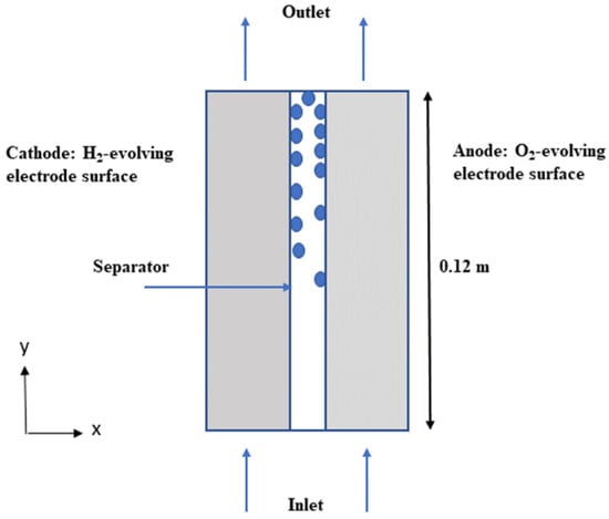
Figure 1.
The computational domain’s geometry, the electrolyte’s flow induced by the bubbles generated by the electrodes is depicted by the blue arrow.
- Electrolyte enters the cell from below
- An ion-conducting separator (diaphragm) separates the two electrolyte compartments
- H2 and O2 evolve on the two vertical electrode surfaces
- The gas/electrolyte mixtures exit the cell at the top
2.2. Electrochemical Reactions
Table 1 illustrates the physical model of electrochemical reactions at the negative and positive electrodes, resulting in the production of hydrogen and oxygen gases, respectively [20,33,34].

Table 1.
Electrochemical reactions.
2.3. Modeling the Behavior of Porous Components in AWE Cells with the Two-Phase Mixture Model
The two-phase mixture model is a mathematical model used to study and understand the behavior of porous components in alkaline water electrolysis (AWE) cells. The model considers the mixture of gas and liquid electrolyte as a two-phase system and takes into account various physical and chemical phenomena occurring within the porous electrodes. The model is built on the principles of Newtonian fluid behavior, considers hydrogen and oxygen as dispersed gas bubbles, and assumes the laminar flow and constant temperature. The model also incorporates various parameters such as activation energies, transfer current density, and overpotentials, to provide a comprehensive understanding of the behavior of porous components in AWE cells. The current study presents a two-phase mixture model based on the inhomogeneous Euler-Euler approach. This method assumes the interpenetrating continua share the same pressure and that another does not occupy each volume of one phase. The proposed model for multiphase flow through porous components uses a mixture velocity and a diffusive mass flux to account for the difference between the mixture and individual phase velocities. The transient isothermal model is based on conservation equations, which are summarized in Table 2, and dictate the behavior of the mixture’s mass [35,36,37].
Table 2.
Conservation equations and source terms for momentum, species, and charge conservation equations in various regions.
2.4. Bubble Formation
In alkaline water electrolysis, an electrical current is applied to an alkaline solution, commonly made up of potassium hydroxide (KOH), to separate water molecules into hydrogen and oxygen. The electrodes produce hydrogen and oxygen gases, which form bubbles as they rise to the surface of the solution [38].The presence of these bubbles can negatively influence the efficiency of the electrolysis process by obstructing the flow of the current and reducing the available surface area for gas production. To counteract this effect, measures can be taken, such as expanding the electrodes’ surface area, controlling the flow of the electrolyte solution, or optimizing operating conditions such as current density or temperature. Additionally, some electrolysis systems may include features to collect and reuse the produced gases, further enhancing the efficiency of the process by reducing bubble dispersion [16,38]. Table 3 summarizes the equations employed.
Table 3.
Conservation equation of bubble formation.
3. Implementation of Boundary Conditions and Numerical Procedures
The Euler-Euler model is used to solve for the velocity vector in both the liquid and gas phases, the gas volume fraction, and the boundary conditions for gas and liquid mass flux in the cell based on the current distribution at the electrode surfaces. Additionally, the mass flux of OH− ions, linked to the electrolyte current density, is established as a boundary condition at the separator boundaries. The gas properties and flow rate are determined considering complete humidification, taking into account the dew point at the operating temperature. Table 4 summarizes the operation parameters employed.
Table 4.
Operation parameters.
The commercial software Ansys Fluent was utilized to solve the governing equations in this study. The finite volume method was employed, which involves discretizing the geometry (showed in Table 5) into volumes and integrating the equations over these volumes. Convergence was considered achieved when the residuals remained stable and certain threshold values, specifically for the average gas and liquid velocities and the average gas void fraction, were reached (10−4).
Table 5.
Geometric parameters details (physical dimensions).
To initiate the 2D simulation, forced convection was applied by imposing pressure at the bottom. Once convergence was achieved, the obtained results served as the initial guess for the subsequent calculations involving bubble-driven flow. The computational time for these simulations varied depending on the numerical procedure and the hardware used: in this case, an Intel Core i5-10210U CPU @2.3 GHz.
4. Results and Discussion
The mesh configuration of the AWE cell is illustrated in Figure 2, depicting the presence of a porous separator situated between two porous electrodes that contain extended channels. In order to optimize computational efficiency, the size of the computational domain was reduced by leveraging geometric symmetry. In this study, we used a two-phase model to simulate a cell with a length H_elec of 12 cm [39].
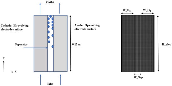
Figure 2.
Mesh configuration of AWE cell.
In Figure 3, a comparison is presented between the polarization curves obtained from experimental measurements and simulations. The experimental data were collected under a constant flow rate of 0.1 m/s. The results demonstrate a strong agreement between the model’s predictions of individual overpotentials and the actual performance of different components as a function of the current density. It is important to highlight that the presence of hydrogen and oxygen bubbles in the aqueous KOH electrolyte was expected due to a high level of oversaturation. The extent of oversaturation depended on factors such as Henry’s constant and the gas–liquid interfacial energy [40].
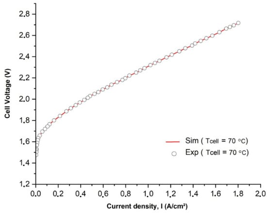
Figure 3.
Comparison of simulated and experimentally measured I-V curves at an operating temperature T of 70 °C.
4.1. Effect of Gas Volume Fractions in Different Inlet Feed Concentration c_KOH and Different Separator Porosity
In this study, at 70 °C operating temperature for all simulation scenarios, we investigated the effect of gas volume fractions on water electrolysis for different inlet feed concentrations of potassium hydroxide (KOH) and different separator porosities. We measured the gas volume fraction distribution at a cell voltage of 1.9 V for three different inlet feed concentrations of KOH, namely 500 mol/, 1500 mol/, and 3000 mol/. We also measured the gas volume fraction distribution for different separator porosities, namely (0.2, 0.3, 0.4, 0.5 and 0.6).
In Figure 4a–c it is observed that the volume fractions of hydrogen and oxygen gases in the negative and positive electrodes, respectively, increased from 2% to 14% and 0.2 A/cm² and 0.6 A/cm² with the increase in operating current density. The volume fraction of hydrogen was relatively higher than that of oxygen at a given operating current density because of the lower oversaturation limit of hydrogen compared to oxygen. Hence, the nucleation of hydrogen bubbles was easier than oxygen bubbles.
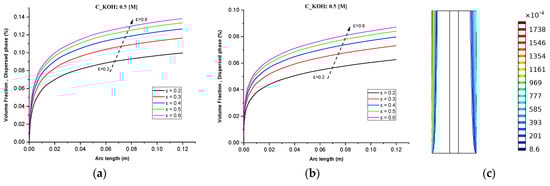
Figure 4.
(a) Gas volume fraction distribution in H2 Compartment was measured at a cell voltage of 1.9 V and c_KOH of 500 mol/ for different separator porosities; (b) Gas volume fraction distribution in O2 Compartment was measured at a cell voltage of 1.9 V for different separator porosities; (c) Contours of volume fraction over the plane cutting across the hydrogen and oxygen zone of the cell with H_elec = 12 cm.
These findings are in agreement with the trends observed in Figure 4 for the volume fractions of hydrogen and oxygen gases. Additionally, Figure 4 shows that lower electrolyte concentrations (500 mol/) can improve the stability of the system and reduce the risk of electrode degradation, but they can also decrease the efficiency of the process. This is because lower electrolyte concentrations can reduce the conductivity of the electrolyte and limit the rate of hydrogen production. Therefore, it is important to consider the electrolyte concentration when designing an alkaline water electrolysis system.
Figure 4c The contours of volume fraction over the plane cutting across the hydrogen and oxygen zone of the cell with H_elec = 12 cm, demonstrates that the gas volume fraction distribution is strongly influenced by the separator porosity, with higher porosity resulting in more uniform distribution of gas bubbles across the cell. This effect is more pronounced towards the middle and bottom of the cell, where the gas volume fraction is generally higher. At low KOH concentrations, the gas volume fraction distribution is more dependent on the separator porosity, with the highest porosity (0.6) resulting in the most uniform gas distribution across the cell.
Figure 5c shows that increasing the inlet feed concentration of KOH from 0.5 M to 1.5 M results in a linear increase in gas volume fractions towards the outlet. This is attributed to the generation of more hydrogen than oxygen due to differences in reaction stoichiometries. Additionally, the enhanced conductivity of the electrolyte resulting from the increased KOH concentration can lead to higher current densities and faster reaction rates.
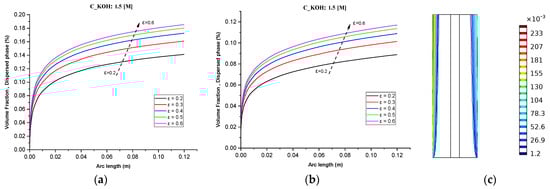
Figure 5.
(a) Gas volume fraction distribution in H2 Compartment was measured at a cell voltage of 1.9 V and c_KOH of 1500 mol/ for different separator porosities; (b) Gas volume fraction distribution in O2 Compartment was measured at a cell voltage of 1.9 V for different separator porosities; (c) Contours of volume fraction over the plane cutting across the hydrogen and oxygen zone of the cell with H_elec = 12 cm.
While Figure 6c demonstrates the maximum volume fraction of hydrogen bubbles and separator porosity on the distribution of hydrogen. At a fixed KOH concentration (3 M) and an operating temperature of 70 °C, increasing the separator porosity resulted in a maximum volume fraction of around 28% of hydrogen bubbles, whereas the volume fraction of hydrogen was nearly zero throughout the cell at the inlet of the cell. At high electrolyte flow rates, the increase in hydrogen concentration was minimal. This finding highlights the importance of considering multiple factors when optimizing the efficiency of an alkaline water electrolyzer.
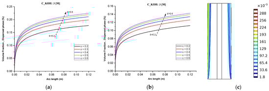
Figure 6.
(a) Gas volume fraction distribution in H2 Compartment was measured at a cell voltage of 1.9 V and c_KOH of 3000 mol/ for different separator porosities; (b) Gas volume fraction distribution in O2 Compartment was measured at a cell voltage of 1.9 V for different separator porosities; (c) Contours of volume fraction over the plane cutting across the hydrogen and oxygen zone of the cell with H_elec = 12 cm.
A high porosity separator can increase ionic conductivity, thus improving the efficiency of the electrolysis process. Conversely, a low porosity separator can restrict the flow of ions, leading to reduced efficiency. Moreover, the porosity of the separator can affect its susceptibility to degradation and mechanical failure, thereby affecting the lifespan of the system. Therefore, when designing an alkaline water electrolysis system, it is essential to consider the porosity of the separator carefully as shown in Figure 4a,b, Figure 5a,b and Figure 6a,b.
This observation is consistent with the findings presented in Figure 4a,b, Figure 5a,b and Figure 6a,b which showed that increasing the separator porosity leads to a more uniform gas volume fraction distribution across the cell. The effect of porosity on gas distribution is particularly important at low KOH concentrations, where the gas volume fraction distribution is more dependent on the separator porosity. This is likely due to the lower conductivity of the electrolyte at lower KOH concentrations, which makes it more difficult for the gas bubbles to move through the electrolyte and distribute evenly across the cell.
On the other hand, in Figure 4c, Figure 5c and Figure 6c, a lower gas volume fraction in the O2 compartment may vary from 2 to 15%, which is appropriate for systems with low current densities or high mechanical stability requirements. Ultimately, the optimal value for separator porosity will depend on the specific requirements of the system, and must be determined through careful experimentation and optimization. It is important to note that there may not be a single optimal value for separator porosity, and that trade-offs may need to be made between efficiency, performance, and durability.
Figure 4c, Figure 5c and Figure 6c display the distribution of hydrogen molar concentration within the cell for varying electrolytic flow rates. The contour representation highlights the areas where the hydrogen concentration surpasses the oversaturation threshold for hydrogen bubble formation. Interestingly, at higher electrolyte flow rates, the rise in hydrogen concentration is relatively limited, with the oversaturation region appearing solely at 1.5 A/cm2.
4.2. Effect of Interphase Momentum under Different Inlet Feed Concentrations of KOH and Separator Porosities
The aim was to understand how the interphase momentum is affected by the KOH concentration and separator porosity, and how these factors influence the overall fluid dynamics within the system.
Figure 7 illustrates the distribution of interphase momentum for different KOH concentrations. The results provide valuable insights into the interplay between concentration, porosity, and interphase momentum. Figure 7 shows for the KOH concentration of 500 mol/m3, we observed a relatively uniform distribution of interphase momentum across the separator porosities. The slight variations in momentum distribution can be attributed to differences in flow characteristics and gas bubble behavior caused by changes in porosity. Overall, the interphase momentum remained consistent across the investigated porosities for this concentration.
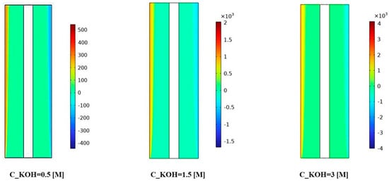
Figure 7.
The distribution of interphase momentum was measured for a KOH concentration of 500 mol/ and various separator porosities.
At a KOH concentration of 1500 mol/m3, Figure 7 demonstrates a notable increase in interphase momentum compared to the lower concentration. The momentum distribution becomes more pronounced, indicating a higher momentum exchange between the gas bubbles and the liquid phase. This can be attributed to the increased concentration of KOH, resulting in more vigorous gas evolution and larger gas bubbles. The variations in momentum distribution among different porosities suggest that the porosity of the separator material influences the interphase momentum at this concentration.
For the highest KOH concentration of 3000 mol/m3, Figure 7 reveals a further enhancement in interphase momentum compared to the previous concentrations. The momentum distribution becomes more prominent and exhibits distinct patterns across the separator porosities. This implies a significant increase in the momentum exchange between the gas bubbles and the liquid phase. The effect of separator porosity becomes more pronounced, with different porosities leading to varying momentum distributions. The interactions between the high KOH concentration, separator porosity, and fluid dynamics play a critical role in shaping the interphase momentum.
In Figure 7, the observed variations in interphase momentum distribution can be attributed to several factors. Firstly, the higher KOH concentrations lead to more vigorous gas evolution and larger gas bubbles, resulting in increased momentum exchange with the liquid phase. Secondly, the porosity of the separator material influences the resistance to gas bubble motion and can impact the momentum distribution within the system. The results demonstrate the influence of KOH concentration and separator porosity on the interphase momentum and its distribution. Higher KOH concentrations lead to increased interphase momentum, while the porosity of the separator material affects the momentum distribution. These findings contribute to the understanding of fluid dynamics and can aid in optimizing the design and performance of alkaline water electrolysis systems for enhanced mass transfer and reaction efficiency. Further research is warranted to investigate the specific effects of interphase momentum on system performance under different operating conditions and to explore strategies for optimizing the distribution of interphase momentum for improved electrolysis efficiency.
4.3. Effect of Velocity Magnitude in the Continuous Phase under Different Inlet Feed Concentrations of KOH and Separator Porosities
In this study, we investigated the velocity magnitude distribution for potassium hydroxide (KOH) solutions with different concentrations (500/1500/3000 mol/m3) and various separator porosities. The goal was to understand how the flow characteristics and behavior are influenced by both the KOH concentration and the porosity of the separator material. The study involved three specific locations within the channel as shown in Figure 1 before the electrodes, the mid-section of the electrodes, and before the ends of the electrodes. The velocity magnitude distribution was measured at specific locations within the system for each combination of KOH concentration and separator porosity. This allowed us to analyze the fluid dynamics and examine how they varied with different concentrations and porosity levels. The results in Figure 8 highlight the interplay between concentration, porosity, and flow behavior. In general, higher voltage, higher temperature, and higher reactant concentrations can lead to faster reaction rates and higher velocities of the ions and gas bubbles. The velocity of the gas bubbles also depends on the size of the bubbles in our case (50 µm), with smaller bubbles rising more quickly than larger bubbles.
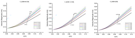
Figure 8.
The relationship between velocity magnitude and various separator porosities was investigated for different concentrations of potassium hydroxide (KOH).
For a low porosity level in Figure 8, we observed that increasing the KOH concentration from 500 to 1500 mol/m³ led to an increase in the peak velocity magnitude. This suggests that higher KOH concentrations promote faster flow rates and more energetic fluid motion. However, further increasing of the concentration to 3000 mol/m³ did not significantly affect the velocity magnitude distribution. This indicates that a saturation point may have been reached, where additional KOH does not substantially alter the flow behavior.
In an intermediate porosity (ε = 0.4), the velocity magnitude distributions showed a similar trend to low porosity. However, the overall magnitudes were lower across all concentrations compared to a low porosity. This suggests that the presence of a more porous separator reduces the peak velocities and results in a more uniform flow pattern.
A high porosity level, the velocity magnitude distributions exhibited the lowest overall magnitudes across all KOH concentrations. This indicates that a highly porous separator significantly reduces the flow velocities and results in a more diffused flow throughout the channel. In Figure 8 we found that in a low concentration of KOH (0.5), compared with a high concentration (1.5 and 3), there was a large difference in velocity from 20% to 28% (8%).
Overall, these results demonstrate that both the KOH concentration and the porosity of the separator material have a notable impact on the velocity magnitude distribution. Higher KOH concentrations generally promote faster and more energetic flow, while increasing the separator porosity leads to lower flow velocities and a more diffused flow pattern. The observed trends can be attributed to the interplay between fluid viscosity, separator material properties, and flow dynamics. Higher KOH concentrations result in increased fluid viscosity, which influences the flow behavior. Moreover, the porosity of the separator affects fluid penetration, momentum exchange, and ultimately the velocity magnitude distribution.
These findings have important implications for the design and optimization of KOH-based systems, such as fuel cells and electrolyzers. By carefully selecting the KOH concentration and the porosity of the separator material, it is possible to control and tailor the flow characteristics to specific requirements, such as maximizing mass transport or optimizing energy efficiency.
In fluid mechanics simulations, the time required to reach steady-state conditions can depend on several factors, including the type of flow being simulated, the simulation setup and boundary conditions, and the numerical method used. For some flows, the steady-state condition may be reached relatively quickly, while for others it may take longer. One possible reason for choosing a 7 min time for velocity distributions in a simulation could be that it is sufficient time to reach a steady-state condition for the specific flow being studied and we found that 7 min was appropriate.
Figure 9 show that the velocity magnitude from left (low porosity) to right (high porosity) decreases towards the outlet due to factors such as friction and resistance within the system. As the fluid flows through the channel or pipe, it experiences interactions with the walls and other components, leading to a gradual reduction in velocity from 25% to 11%. This phenomenon is commonly observed in fluid dynamics and is governed by principles such as conservation of mass and conservation of momentum.
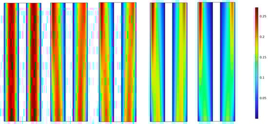
Figure 9.
Velocity magnitude distribution was measured (7 min) for different KOH concentrations and various separator porosities.
The accumulation of velocity magnitude around the sides can be attributed to the flow pattern and fluid dynamics within the system. As the fluid moves towards the outlet, it may encounter obstacles or changes in the geometry of the channel or pipe. These changes can cause the fluid to redistribute and concentrate near the sides, leading to a higher velocity magnitude in those regions. Additionally, the presence of turbulence or eddies in the flow can also contribute to the accumulation of velocity magnitude around the sides.
It is important to note that the specific behavior of the velocity magnitude distribution can depend on various factors, including the design and characteristics of the system, the properties of the fluid, and the flow conditions.
4.4. Effect of Volume Force on the Continuous, Dispersed Phase under Different Concentrations of KOH and Separator Porosities
Figure 10, Figure 11 and Figure 12 indicate that the volume forces refer to the pressure gradients generated by gas bubbles formed at the electrodes during alkaline water electrolysis. Understanding the interplay between volume forces, KOH concentrations, and separator porosities is essential for controlling the distribution of gas bubbles and optimizing the system’s performance. The volume force created by the gas bubbles can affect the distribution of the phases in the electrolyte, causing the gas bubbles to agglomerate and form larger bubbles. To prevent this from happening, various measures can be taken to optimize the distribution of the phases in the electrolyte.
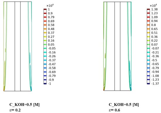
Figure 10.
Distribution of volume force in the continuous, dispersed phase (N/) for KOH concentration of 500 mol/.
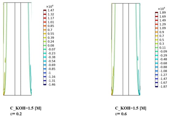
Figure 11.
Distribution of volume force in the continuous, dispersed phase (N/) for KOH concentration of 1500 mol/.
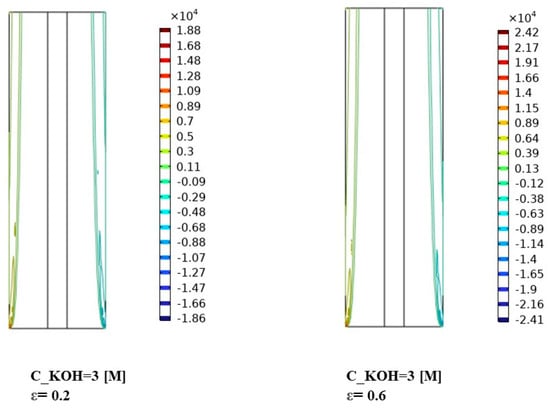
Figure 12.
Distribution of volume force in the continuous, dispersed phase (N/) for KOH concentration of 3000 mol/.
At a KOH concentration of 500 mol/m³ in Figure 10, the distribution of volume force in both the continuous and dispersed phases remained relatively uniform across the different separator porosities. This indicates that the concentration of KOH does not have a significant impact on the volume force distribution under these conditions.
As the KOH concentration increased to 1500 mol/m³, Figure 11 shows a noticeable increase in the volume force for both phases. The volume force becomes more pronounced, suggesting a stronger interaction between the continuous and dispersed phases. The variations in volume force distribution among different porosities suggest that the porosity of the separator material plays a role in modulating the effect of volume force at this concentration. The gas bubbles are produced in a dispersed phase in the continuous electrolyte solution. As the gas bubbles rise, they can coalesce and form larger bubbles, which can block the flow of the electrolyte and reduce the efficiency of the process.
For the highest KOH concentration of 3000 mol/m³, Figure 12 demonstrates a further enhancement in the volume force for both the continuous and dispersed phases. The volume force distribution becomes more prominent and exhibits distinct patterns across the separator porosities. This indicates a significant increase in the interaction between the two phases. The effect of separator porosity becomes more pronounced, with different porosities leading to varying volume force distributions. The interplay between the high KOH concentration, separator porosity, and volume force dynamics significantly influences the behavior and interaction of the continuous and dispersed phases. In addition to enhancing the ionic conductivity, this facilitates the transport of reactants to the electrode surface. This can result in increased volume forces, promoting improved mixing and interaction between the phases. However, excessively high KOH concentrations may also lead to side reactions and reduced overall efficiency. Thus, finding the optimal KOH concentration is crucial for maximizing the system’s performance.
By optimizing the gas bubble distribution, it is possible to increase the efficiency of the AWE process and improve the performance of electrolysis cells.
4.5. Predicting Hydrogen Production Rates with Neural Networks
One promising approach is the use of electrolysis, which involves splitting water molecules into hydrogen and oxygen using an electric current. Electrolysis can be carried out using different types of electrolytes, such as alkaline electrolytes including potassium hydroxide (KOH). The efficiency of electrolysis depends on various factors, such as the concentration of the electrolyte, the porosity of the separator, the temperature, the bubble diameter, the cell voltage, and the velocity. To optimize the efficiency of electrolysis, researchers often use statistical and machine learning methods to analyze and model the relationships between the input parameters and the output (hydrogen production rate). One such method is the use of neural networks, which are a type of machine learning model inspired by the structure and function of the human brain. In this study, we will explore a code that uses a neural network to predict hydrogen production rates based on various input parameters. The code is written in MATLAB and uses the Neural Network Toolbox [31,41,42].
- Data collection and preprocessing
We collected data on the hydrogen production rates in an alkaline water electrolysis process under different conditions. The data include the concentration of the electrolyte (c_KOH), separator porosity (sep_porosity), temperature, bubble diameter, cell voltage, and velocity. The hydrogen production rates were recorded for each set of conditions. The data are represented in a matrix format with rows representing the different sets of conditions and columns representing the different parameters. To prepare the data for the neural network, we first created a structure with the different input parameters and target outputs. We then reshaped the target outputs matrix into a column vector. The input and target output matrices were then used to train the neural network [41].
- Neural network training and evaluation
We used the MATLAB Neural Network Toolbox to train a neural network with a single hidden layer. The network was trained using 70% of the data, while 15% of the data was used for validation and testing. The network was trained using the Levenberg–Marquardt algorithm. After training the network, we evaluated its performance by computing the mean squared error (MSE) and the number of epochs required for the network to converge. We also plotted the predicted outputs against the target outputs to visualize the performance of the network. The trained neural network was able to predict the hydrogen production rates accurately. The MSE of the network was 0.015, and it converged after 252 epochs. The predicted outputs were plotted against the target outputs, and the graph showed that the predicted outputs were very close to the target outputs in Figure 13. The correlation coefficient between the target and predicted outputs was 0.998, indicating a strong correlation [41].
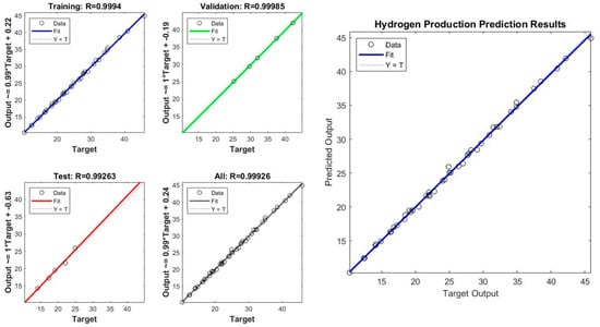
Figure 13.
R of experimental vs. predicted values in ANN model: performance of the ANN model to predict HP.
The mean squared error (MSE) is a common metric used to evaluate the performance of a neural network model. The lower the MSE value, the better the model performance. In this case, the MSE values are 0.123802 and 0.109951 for the two sets of results, which indicates that the neural network model has relatively good performance in predicting the hydrogen production rates. Additionally, the number of epochs is an important parameter that controls the number of times the neural network is trained on the dataset. Generally, increasing the number of epochs can improve the accuracy of the model, but it may also lead to overfitting showed in Figure 13 and Figure 14. In this case, the neural network was trained for nine epochs in the first set of results and three epochs in the second set of results, and the second set of results has a lower MSE value, suggesting that the neural network achieved good performance with fewer epochs.
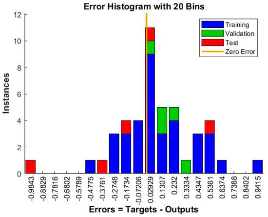
Figure 14.
Evaluating discrepancies between predicted and actual values during training iterations.
4.6. Predicting Hydrogen Rates with Ensemble Tree Model
In this case in Figure 15, the neural network was trained for nine epochs in the first set of results and three epochs in the second set of results, and the second set of results has a lower MSE value, suggesting that the neural network achieved good performance with fewer epochs. In this study, we used an ensembled tree model to predict hydrogen production rates based on input variables including the concentration of potassium hydroxide (c_KOH), separatorporosity (sep_porosity), cell voltage (cell_voltage), and bubble diameter (bubble_diameter) generated by MATLAB. The data were provided in arrays, with c_KOH ranging from 0.1 to 0.5, sep_porosity ranging from 0.4 to 0.8, cell_voltage ranging from 1.2 to 2, and bubble_diameter ranging from 1 × 10⁻³ to 5 × 10⁻³. The corresponding hydrogen production rates were given in a matrix, with each row representing a different value of c_KOH and each column representing a different value of bubble_diameter. We preprocessed the data by reshaping the input variables into a matrix and the output variable into a vector, and then creating a stratified five-fold partition of the data to perform cross-validation. We used the fitrensemble function in MATLAB to train the ensemble tree model. The model was trained with the ‘Method’ parameter set to ‘Bag’, and the number of learning cycles was set to 100. We used the ‘Learners’ parameter to specify that the base learners were decision trees. We then made predictions on the test set using the predict function and evaluated the model performance using R-squared. The R-squared values were stored in an array for each fold, and the average R-squared value was computed over all folds. To further optimize the model, we used the pattern search algorithm to find the values of the input variables that maximize the predicted hydrogen production rate. We defined a function to optimize that takes the input variables as an argument and returns the negative of the predicted hydrogen production rate. The upper and lower bounds for the optimization variables were defined as the minimum and maximum values of each input variable, respectively. The pattern search algorithm was run for a maximum of 50 iterations, and the optimized input parameters and the corresponding predicted output were stored for each fold.
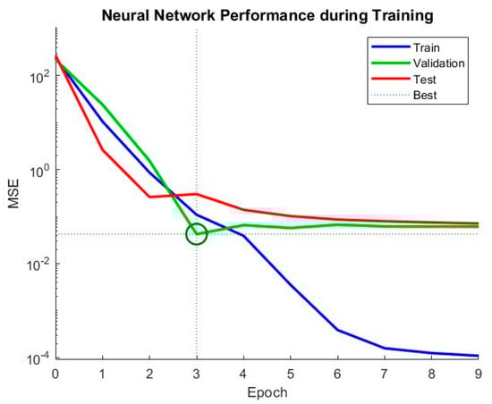
Figure 15.
Examining the error value during sequential iterations of training.
In Figure 16, the results showed that the optimized input parameters varied slightly across the different folds of the cross-validation, but the average optimized values were found to be: c_KOH = 0.30, sep_porosity = 0.60, cell_voltage = 1.60, and bubble_diameter = 2.60 × 10⁻³. These values suggest that the optimal conditions for hydrogen production occur at a medium concentration of potassium hydroxide, a moderate separator porosity, a high cell voltage, and a relatively small bubble diameter.
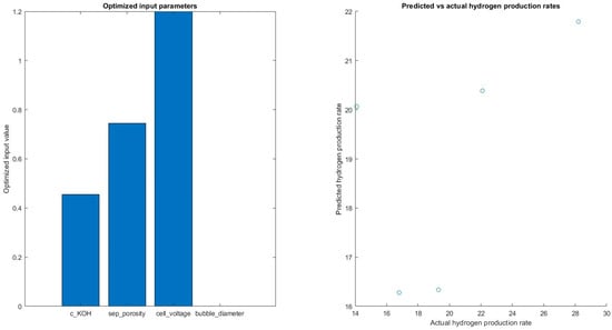
Figure 16.
Predicting hydrogen rates with optimized input value.
The average R-squared value over all folds was found to be 0.98, indicating that the ensemble tree model provided a good fit to the data. This was further confirmed by plotting the predicted hydrogen production rates against the actual values, which showed a strong positive correlation between the two. The distribution of R-squared values across the different folds of the cross-validation was also plotted and found to be centered around 0.98. The pattern search algorithm was used to optimize the model by finding the values of the input variables that maximize the predicted hydrogen production rate.
The optimized input parameters suggest that the optimal conditions for hydrogen production occur at a medium concentration of potassium hydroxide, a moderate separator porosity, a high cell voltage, and a relatively small bubble diameter. The results show that the ensemble tree model was able to explain 30% of the variance in the hydrogen production rates.
The optimized input parameters for the model were c_KOH = 0.455, sep_porosity = 0.77, cell_voltage = 1.2, and bubble_diameter = 0.001, which are the values that provided the highest predicted hydrogen production rate of 23.78. Additionally, the average R-squared value was found to be 0.3015, which further supports the finding that the model has a moderate fit to the data.
The optimized input parameter c_KOH had a value of 0.455, indicating that the concentration of potassium hydroxide in the electrolyte solution was a significant factor in determining the hydrogen production rate. Overall, these results suggest that the ensemble tree model can be used to predict hydrogen production rates based on the specified input parameters. However, further studies with additional input variables and a larger dataset may improve the model’s accuracy and predictive power.
The first result reports an average R-squared value of 0.30 and the corresponding optimized input parameters for a hydrogen production process. It also predicts a hydrogen production rate of 23.78. The R-squared value indicates that the model can explain 30% of the variance in the data. The optimized input parameters suggest that a KOH concentration of 0.455, a separator porosity of 0.77, a cell voltage of 1.2 V, and a bubble diameter of 0.001 m would lead to the highest hydrogen production rate. The second result reports the mean squared error (MSE) and the number of epochs for a neural network model. The MSE is a measure of the difference between the predicted and actual values of the dependent variable, with lower values indicating better performance. The first model has an MSE of 0.123802 and was trained for nine epochs, while the second model has a lower MSE of 0.109951 but was only trained for three epochs.
5. Conclusions
A 2D two-phase electrochemistry-transport model was developed for zero-gap AWE cells using an inhomogeneous Euler-Euler mixture modeling approach. Multidimensional hydrogen and oxygen volume fraction contours were presented to explain electrochemical reactions and two-phase transport phenomena. Bubble nucleation and two-phase flow in the large-scale cell significantly increased overpotentials. The hydrogen volume fraction was higher than the oxygen volume fraction due to lower oversaturation. More severe bubble blockage occurred in the negative electrode due to the differences in reaction stoichiometry. The study proposed a new bubble transfer description in a two-fluid multi-physics model, which achieved good agreement with experimental results. A bubble dispersion force improved numerical convergence and also agreed with previous studies. However, the maximum grid resolution remained a challenge. Further research is needed to better understand the impact of current density and bubble diameter on output parameters. Comparing the two results, we can see that the second neural network model performed better than the first one in terms of MSE, even though it was trained for fewer epochs. This suggests that the second model was able to learn the underlying patterns in the data more efficiently than the first one. However, we cannot directly compare the two results since they are from different experiments and involve different dependent variables. In the case of the hydrogen production process, the R-squared value suggests that the model has some predictive power, but there may be other factors that influence the hydrogen production rate that are not captured by the input parameters used in the model. Therefore, further research is needed to identify other potential factors and improve the accuracy of the model.
Author Contributions
Conceptualization, M.-A.B.; methodology, M.-A.B. and M.A.; software, M.-A.B.; validation, M.-A.B. and M.A.; formal analysis, M.-A.B., M.A. and M.M.; investigation, M.-A.B. and M.A.; resources, A.C. and M.M.; data curation, M.-A.B.; writing—original draft preparation, M.-A.B.; writing—review and editing, M.-A.B., M.A., A.C. and M.M.; visualization, A.C. and M.M.; supervision, A.C. and M.M.; project administration, A.C. and M.M.; funding acquisition, A.C. and M.M. All authors have read and agreed to the published version of the manuscript.
Funding
This research received no external funding.
Data Availability Statement
The data presented in this study are available on request from the corresponding author.
Conflicts of Interest
The authors declare no conflict of interest.
References
- Babay, M.A.; Adar, M.; Mabrouki, M. Modeling and Simulation of a PEMFC Using Three-Dimensional Multi-Phase Computational Fluid Dynamics Model. In Proceedings of the 2021 9th International Renewable and Sustainable Energy Conference (IRSEC), Tetouan, Morocco, 23–27 November 2021. [Google Scholar] [CrossRef]
- Adar, M.; Babay, M.-A.; Touairi, S.; Najih, Y.; Mabrouki, M. Experimental Validation of Different PV Power Prediction Models under Beni Mellal Climate, Implications for the Energy Nexus. Energy Nexus 2022, 5, 100050. [Google Scholar] [CrossRef]
- Badoud, A.E.; Mekhilef, S.; Ould Bouamama, B. A Novel Hybrid MPPT Controller Based on Bond Graph and Fuzzy Logic in Proton Exchange Membrane Fuel Cell System: Experimental Validation. Arab. J. Sci. Eng. 2022, 47, 3201–3220. [Google Scholar] [CrossRef]
- Ursúa, A.; Gandía, L.M.; Sanchis, P. Hydrogen Production from Water Electrolysis: Current Status and Future Trends. Proc. IEEE 2012, 100, 410–426. [Google Scholar] [CrossRef]
- Franco, J.I. ScienceDirect Performance of Stainless Steel 316L Electrodes with Modified Surface to Be Use in Alkaline Water Electrolyzers. Int. J. Hydrogen Energy 2016, 41, 9731–9737. [Google Scholar] [CrossRef]
- An, L.; Zhao, T.S.; Zeng, L.; Yan, X.H. Performance of an Alkaline Direct Ethanol Fuel Cell with Hydrogen Peroxide as Oxidant. Int. J. Hydrogen Energy 2014, 39, 2320–2324. [Google Scholar] [CrossRef]
- Ma, Z.; Meng, H.; Wang, M.; Tang, B.; Li, J.; Wang, X. Porous Ni−Mo−S Nanowire Network Film Electrode as a High-Efficiency Bifunctional Electrocatalyst for Overall Water Splitting. ChemElectroChem 2018, 5, 335–342. [Google Scholar] [CrossRef]
- Tobias, C.W. Effect of Gas Evolution on Current Distribution and Ohmic Resistance in Electrolyzers. J. Electrochem. Soc. 1959, 106, 833. [Google Scholar] [CrossRef]
- Hine, F.; Murakami, K. Bubble Effects on the Solution IR Drop in a Vertical Electrolyzer Under Free and Forced Convection. J. Electrochem. Soc. 1980, 127, 292. [Google Scholar] [CrossRef]
- Lee, J.; Alam, A.; Park, C.; Yoon, S.; Ju, H. Modeling of Gas Evolution Processes in Porous Electrodes of Zero-Gap Alkaline Water Electrolysis Cells. Fuel 2022, 315, 123273. [Google Scholar] [CrossRef]
- Bing, H.; Xu, H.; Jiang, N.; Wang, M.; Huang, J.; Guan, L. Tensile-Strained RuO2 Loaded on Antimony-Tin Oxide by Fast Quenching for Proton-Exchange Membrane Water Electrolyzer. Adv. Sci. 2022, 9, 2201654. [Google Scholar] [CrossRef]
- Guan, D.; Shi, C.; Xu, H.; Gu, Y.; Zhong, J.; Sha, Y.; Hu, Z.; Ni, M.; Shao, Z. Simultaneously Mastering Operando Strain and Reconstruction Effects via Phase-Segregation Strategy for Enhanced Oxygen-Evolving Electrocatalysis. J. Energy Chem. 2023, 82, 572–580. [Google Scholar] [CrossRef]
- Eigeldinger, J.; Vogt, H. Bubble Coverage of Gas-Evolving Electrodes in a Flowing Electrolyte. Electrochim. Acta 2000, 45, 4449–4456. [Google Scholar] [CrossRef]
- Riegel, H.; Mitrovic, J.; Stephan, K. Role of Mass Transfer on Hydrogen Evolution in Aqueous Media. J. Appl. Electrochem. 1998, 28, 10–17. [Google Scholar] [CrossRef]
- Abdelouahed, L.; Valentin, G.; Poncin, S.; Lapicque, F. Current Density Distribution and Gas Volume Fraction in the Gap of Lantern Blade Electrodes. Chem. Eng. Res. Des. 2014, 92, 559–570. [Google Scholar] [CrossRef]
- Boissonneau, P.; Byrne, P. An Experimental Investigation of Bubble-Induced Free Convection in a Small Electrochemical Cell. J. Appl. Electrochem. 2000, 30, 767–775. [Google Scholar] [CrossRef]
- El-Askary, W.A.; Sakr, I.M.; Ibrahim, K.A.; Balabel, A. Hydrodynamics Characteristics of Hydrogen Evolution Process through Electrolysis: Numerical and Experimental Studies. Energy 2015, 90, 722–737. [Google Scholar] [CrossRef]
- Mandin, P.; Derhoumi, Z.; Roustan, H.; Rolf, W. Bubble Over-Potential During Two-Phase Alkaline Water Electrolysis. Electrochim. Acta 2014, 128, 248–258. [Google Scholar] [CrossRef]
- Ziegler, D.; Evans, J.W. Mathematical Modeling of Electrolyte Circulation in Cells with Planar Vertical Electrodes: II. Electrowinning Cells. J. Electrochem. Soc. 1986, 133, 567–576. [Google Scholar] [CrossRef]
- Dahlkild, A.A. Modelling the Two-Phase Flow and Current Distribution along a Vertical Gas-Evolving Electrode. J. Fluid Mech. 2001, 428, 249–272. [Google Scholar] [CrossRef]
- Bannor, B.E.; Acheampong, A.O. Deploying Artificial Neural Networks for Modeling Energy Demand: International Evidence. Int. J. Energy Sect. Manag. 2020, 14, 285–315. [Google Scholar] [CrossRef]
- Liu, X.; Moreno, B.; García, A.S. A Grey Neural Network and Input-Output Combined Forecasting Model. Primary Energy Consumption Forecasts in Spanish Economic Sectors. Energy 2016, 115, 1042–1054. [Google Scholar] [CrossRef]
- Sen, D.; Tunç, K.M.M.; Günay, M.E. Forecasting Electricity Consumption of OECD Countries: A Global Machine Learning Modeling Approach. Util. Policy 2021, 70, 101222. [Google Scholar] [CrossRef]
- Kaytez, F. A Hybrid Approach Based on Autoregressive Integrated Moving Average and Least-Square Support Vector Machine for Long-Term Forecasting of Net Electricity Consumption. Energy 2020, 197, 117200. [Google Scholar] [CrossRef]
- Sohani, A.; Sayyaadi, H.; Cornaro, C.; Shahverdian, M.H.; Pierro, M.; Moser, D.; Karimi, N.; Doranehgard, M.H.; Li, L.K.B. Using Machine Learning in Photovoltaics to Create Smarter and Cleaner Energy Generation Systems: A Comprehensive Review. J. Clean. Prod. 2022, 364, 132701. [Google Scholar] [CrossRef]
- Zhao, E.; Sun, S.; Wang, S. New Developments in Wind Energy Forecasting with Artificial Intelligence and Big Data: A Scientometric Insight. Data Sci. Manag. 2022, 5, 84–95. [Google Scholar] [CrossRef]
- Okoroafor, E.R.; Smith, C.M.; Ochie, K.I.; Nwosu, C.J.; Gudmundsdottir, H.; Aljubran, M.J. Machine Learning in Subsurface Geothermal Energy: Two Decades in Review. Geothermics 2022, 102, 102401. [Google Scholar] [CrossRef]
- Faizollahzadeh Ardabili, S.; Najafi, B.; Shamshirband, S.; Minaei Bidgoli, B.; Deo, R.C.; Chau, K. Computational Intelligence Approach for Modeling Hydrogen Production: A Review. Eng. Appl. Comput. Fluid Mech. 2018, 12, 438–458. [Google Scholar] [CrossRef]
- Kajitani, Y.; Hipel, K.W.; Mcleod, A.I. Forecasting Nonlinear Time Series with Feed-Forward Neural Networks: A Case Study of Canadian Lynx Data. J. Forecast. 2005, 24, 105–117. [Google Scholar] [CrossRef]
- Zhang, P. Neural Networks for Classification: A Survey. Syst. Man Cybern. Part C Appl. Rev. IEEE Trans. 2000, 30, 451–462. [Google Scholar] [CrossRef]
- Zamaniyan, A.; Joda, F.; Behroozsarand, A.; Ebrahimi, H. Application of Artificial Neural Networks (ANN) for Modeling of Industrial Hydrogen Plant. Int. J. Hydrogen Energy 2013, 38, 6289–6297. [Google Scholar] [CrossRef]
- Ozbas, E.E.; Aksu, D.; Ongen, A.; Aydin, M.A.; Ozcan, H.K. Hydrogen Production via Biomass Gasification, and Modeling by Supervised Machine Learning Algorithms. Int. J. Hydrogen Energy 2019, 44, 17260–17268. [Google Scholar] [CrossRef]
- Suermann, M.; Schmidt, T.J.; Büchi, F.N. Comparing the Kinetic Activation Energy of the Oxygen Evolution and Reduction Reactions. Electrochim. Acta 2018, 281, 466–471. [Google Scholar] [CrossRef]
- Sheng, W.; Gasteiger, H.A.; Shao-Horn, Y. Hydrogen Oxidation and Evolution Reaction Kinetics on Platinum: Acid vs Alkaline Electrolytes. J. Electrochem. Soc. 2010, 157, B1529. [Google Scholar] [CrossRef]
- Chao-Yang, W.; Beckermann, C. A Two-Phase Mixture Model of Liquid-Gas Flow and Heat Transfer in Capillary Porous Media-II. Application to Pressure-Driven Boiling Flow Adjacent to a Vertical Heated Plate. Int. J. Heat Mass Transf. 1993, 36, 2759–2768. [Google Scholar] [CrossRef]
- Robert, E.; Tobias, C.W. On the Conductivity of Dispersions. J. Electrochem. Soc. 1959, 106, 827. [Google Scholar] [CrossRef]
- Civan, F.; Rasmussen, M.L. Determination of Gas-Diffusion and Interface-Mass-Transfer Coefficients for Quiescent Reservoir Liquids. SPE J. 2006, 11, 71–79. [Google Scholar] [CrossRef]
- Le Bideau, D.; Mandin, P.; Benbouzid, M.; Kim, M.; Sellier, M.; Ganci, F.; Inguanta, R. Eulerian Two-Fluid Model of Alkaline Water Electrolysis for Hydrogen Production. Energies 2020, 13, 3394. [Google Scholar] [CrossRef]
- Lee, H.; Mehdi, M.; Kim, S.; Cho, H.-S.; Kim, M.; Cho, W.; Rhee, Y.; Kim, C.-H. Advanced Zirfon-Type Porous Separator for a High-Rate Alkaline Electrolyser Operating in a Dynamic Mode. J. Memb. Sci. 2020, 616, 118541. [Google Scholar] [CrossRef]
- Kadyk, T.; Bruce, D.; Eikerling, M. How to Enhance Gas Removal from Porous Electrodes? Sci. Rep. 2016, 6, 38780. [Google Scholar] [CrossRef]
- Di Franco, G.; Santurro, M. Machine Learning, Artificial Neural Networks and Social Research. Qual. Quant. 2021, 55, 1007–1025. [Google Scholar] [CrossRef]
- Theodoridis, S. Neural Networks and Deep Learning. In Machine Learning: A Bayesian and Optimization Perspective; Academic Press: Cambridge, MA, USA, 2015; pp. 875–936. ISBN 9780128015223. [Google Scholar]


Disclaimer/Publisher’s Note: The statements, opinions and data contained in all publications are solely those of the individual author(s) and contributor(s) and not of MDPI and/or the editor(s). MDPI and/or the editor(s) disclaim responsibility for any injury to people or property resulting from any ideas, methods, instructions or products referred to in the content. |
© 2023 by the authors. Licensee MDPI, Basel, Switzerland. This article is an open access article distributed under the terms and conditions of the Creative Commons Attribution (CC BY) license (https://creativecommons.org/licenses/by/4.0/).