Abstract
It is very important to perform magnetostatic analysis accurately and efficiently when it comes to multi-objective optimization of designs of electromagnetic devices, particularly for inductors, transformers, and electric motors. A kernel free boundary integral method (KFBIM) was studied for analyzing 2D magnetostatic problems. Although KFBIM is accurate and computationally efficient, sharp corners can be a major problem for KFBIM. In this paper, an inverse discrete Fourier transform (DFT) based geometry reconstruction is explored to overcome this challenge for smoothening sharp corners. A toroidal inductor core with an airgap (C-core) is used to show the effectiveness of the proposed approach for addressing the sharp corner problem. A numerical example demonstrates that the method works for the variable coefficient PDE. In addition, magnetostatic analysis for homogeneous and nonhomogeneous material is presented for the reconstructed geometry, and results carried out using KFBIM are compared with the results of FEM analysis for the original geometry to show the differences and the potential of the proposed method.
1. Introduction
Significant advancements have been made in solving elliptic partial differential equations numerically over the past few decades, especially towards solving magnetostatic problems. The Finite Element Method (FEM) is the prominent numerical method to analyze magnetostatics problems because of its geometric flexibility with complicated shapes of electromagnetic devices, especially electrical machines [1,2,3]. The adaptive and local mesh refinement algorithm is developed and available in commercial software, for example, the AC/DC Module of COMSOL [4] and ANSYS Maxwell of ANSYS [5]. However, the body-fitted unstructured (quality) grids around the surface of the magnetic devices are required to be meshed by the finite element method, especially in three space dimensions, which is usually a difficult, expensive, and time-consuming process.
Boundary element/integral methods (BEM/BIM) were introduced in the electromagnetics domain and have become popular alternative approaches for analyzing magnetic fields [6,7,8]. The boundary integral method is often recognized as the most accurate method since it treats the boundary conditions precisely and provides accurate, stable, and well-developed quadrature of boundary integrals [9,10,11]. This kind of method may be considered the most efficient numerical method theocratically, because this method reduces one dimension of the problem, for example, the computational cost is reduced dramatically if a 2D problem can be solved through the integration of a 1D geometry. For a homogeneous elliptic partial differential equation (PDE), the potential theory is used to reformulate the PDE as a boundary integral equation with the help of Green’s functions, i.e., the solution to the PDE can be described by an integral. Thus, the classical boundary element method (BEM) discretizes the boundaries instead of the whole volume or area, which reduces magnetostatic problems by one dimension, which is the benefit of the BEM. The boundary element/integral method requires computational work that changes linearly with the number of unknowns on the boundary. The boundary element methods (BEM) and the Methods of Moment (MoM) are similar and relatively well-known in the magnetostatic analysis area. Although benefits from these methods are obvious, BEM and MoM have several limitations. First, they are not good candidates for nonlinear problems since it is difficult for them to inherently solve inhomogeneous and nonlinear problems in the domain interior. Second, the evaluation of volume integrals for a partial differential equation with variable coefficients is not straightforward for these methods. Third, for evaluating integrals and solving the problem, the analytic expression of Green’s function is necessary for these methods for all PDE problems. The analysis process for engineers is more complicated because the analytic expressions of Green’s functions is typically impossible to derive for PDEs defined in complex geometry with variable coefficients, and it is hard to derive it analytically even if it exists theoretically in some cases. Finally, but importantly, the boundary element/integral method involves singular and hyper-singular boundary integrals, and improper evaluation of the integrals affects the accuracy and stability of the method. The disadvantages of the BEM are not negligible, but significant progress and special treatments have been made and are still going on [12,13,14].
A new boundary integral method named the Kernel Free Boundary Integral Method (KFBIM) was recently developed and introduced in electromagnetics [15]. The uniqueness of the KFBIM method is that special quadrature, or kernels, are not needed for the evaluation of integrals directly. The kernel is the analytic expression of Green’s functions in KFBIM. The concept behind KFBIM is reinterpreting each volume and boundary integral as results of solving simple equivalent interface problems created in a rectangular domain box. In KFBIM, interface problems are solved by a finite difference method (FDM) coupled with numerical corrections at irregular points and fast Fourier transform (FFT) based solvers and interpolations to obtain efficiency and accuracy. Furthermore, the KFBIM can solve inhomogeneous variable coefficients’ elliptic PDEs. In addition, KFBIM accurately computes singular and hyper-singular boundary integrals that appear in the boundary integral formulation. No special treatments are required to overcome the limitations of the traditional BEM. In addition, different to the FDM, which directly solves a partial differential equation, KFBIM is based on the formulation of integrals, therefore, a well-conditioned discrete linear system of equations is produced by KFBIM. Thus, the sensitivity of KFBIM to computer errors is much lower and more accurate. KFBIM was proposed to be a general method to solve constant or variable elliptic PDEs for single or double boundaries in two or three dimensions [16,17,18,19,20,21,22]. Cartesian grid-based methods are used in KFBIM to solve the integrals, which means a body-fitted mesh is not required to solve the problems and can obtain higher accuracy on a coarser mesh when solving integrals when compared to FEM and BEM. Detailed comparisons of the common numerical methods are shown in Table 1.

Table 1.
Comparison between common numerical methods’ strengths and weaknesses.
Problems with smooth boundaries in electromagnetics in two-dimensions are well understood. It was found that they can be solved by the boundary integral method accurately and efficiently [6,7,8,15]. However, sharp corners can be a problem for integral method analysis—the derivation of integral methods assumes that domain boundaries are smooth in general. At sharp corners, the flux field can be singular (or nearly so) and discontinuous. Such singular behavior affects the accuracy of the numerical methods throughout the whole domain. Sharp corners exist in several applications in the engineering area, especially electromagnetics, such as the rotor pole and stator pole in electrical machines and corners of the inductors and transformers. However, there are almost no smooth boundaries in the applications. Therefore, it must be addressed using some treatments for BIMs. Several special treatments for BEM have been made, mathematically or geometrically [23,24]. However, for KFBIM, there is no special treatment reported yet. In this paper, a geometry reconstruction method to smooth the shape of the boundary is proposed for KFBIM. The zero-padded/filled inverse discrete Fourier transform (iDFT) is used to smooth the boundary, which is commonly seen in image processing. Although this method is used when the data is limited and data extrapolation is needed [25,26,27], it has the effect of removing the sharp edge. After the original boundary is reconstructed by zero-padded/filled IDFT, the sharp corner is removed theoretically.
In this study, a C-core (toroid core with gap) shape with a corner is taken as a magnetostatic analysis example to show the effectiveness of the smooth method. The toroidal core is often used in designs of toroidal transformers and inductors because the inductance of the toroidal core is higher. Most magnetic flux enclosed in the toroidal core leads to higher inductance [28]. Due to the advantages of toroidal transformers and inductorssuch as higher efficiency and inductance, lower flux leakage and lighter weight, they are often used in the following applications: amplifiers, inverters, and power supplies [15]. They are widely used in high power low-frequency power electronics applications. One prime example of such applications is power conversion [29]. The air gap introduces a large amount of magnetic reluctance within the core. The slope of the B–H curve is reduced by the airgap. Therefore, the inductor can handle more current without saturation, compared to the original toroid core, although the saturation flux density does not change. The air-gapped toroid core is only used in power conversion; it is used as a surge protector device [30]. A real air-gapped core is shown in Figure 1.
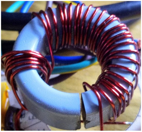
Figure 1.
Toroidal inductor with an air gap [30].
This paper is organized as follows: Partial differential equations governing magnetostatic analysis and inductance calculation of the C-core are presented in Section 2. The Kernel Free Boundary Integral Method framework is derived for single boundary magnetostatic problem analysis in Section 3. Section 4 shows the sharp corner reconstruction technique to smooth the boundary and implementation of the Kernel Free Boundary Integral Method for electromagnetics analysis. Section 5 shows results carried out from the Kernel Free Boundary Integral Method framework compared to the FEM results and includes a discussion of the results. In the last section, the conclusion is drawn, and future studies and potentials are discussed for the sharp corner reconstruction of the Kernel Free Boundary Integral Method for electromagnetic problem analysis.
2. The C-core Problem
2.1. The Dimensions of C-core
The sharp corner reconstruction and magnetostatic problem of the C-core are studied in this paper. Figure 2 shows the rectangular box, coils, and C-core. Table 2 summarizes the dimensions of the C-core geometry. It should be noted that the C-core models in the study are idealized mainly for modeling purposes. Partial differential equations (PDEs), proper boundary conditions (BCs) governing the magnetostatics analysis problem, and the equations of the inductance calculation form the first step in this study presented in Section 2.2 and Section 2.3.
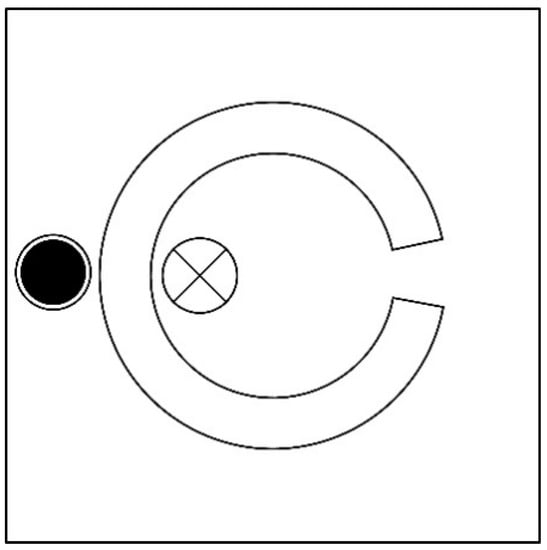
Figure 2.
The C-core geometry.
Table 2.
C-core dimensions.
2.2. PDEs and BCs for Magnetostatic Analysis
The PDEs and BCs are derived from a previous study [26]. The PDE is
where is the magnetic vector potential, is current density, and is denoted as the reciprocal of magnetic permeability. In 2D, it can be rewritten as
where and are current density and magnetic vector potential in the direction. The BC of the boundary of the rectangular air box is
Additionally, a continuity condition of must be satisfied at the air–iron boundaries along the normal direction,
where the and denotes the reciprocal of magnetic permeability of air or vacuum and iron, respectively, and is the outward normal unit vector on each boundary. The continuity of the magnetic vector potential on boundaries between different domains is required to ensure the continuity of the normal vector of magnetic flux density.
2.3. Inductance Calculation
The inductance of this study is analyzed using magnetic energy. For this method, the magnetic energy term is used, for each point, the energy per unit volume is:
Therefore, the magnetic energy is:
In the 2D case, it should be
which is
The relationship between magnetic energy and inductance is
where is inductance, and is the current.
So, in general, the average is calculated from iron and air and then applied to the formula, respectively, to compute the total magnetic energy.
3. KFBIM Framework for Single Boundary Magnetostatic Problems
A general KFBIM framework to solve the single boundary electromagnetic problem is derived in this section. The KFBIM framework is implemented for the C-core magnetostatics problem shown in the next section to study the sharp corner reconstruction method. Similar work has been performed for a toroidal core magnetostatics problem with double boundaries [15]. In this paper, the presented formulation is extended from the method developed in recent years [16] and is reformulated for the single boundary magnetostatics problem. The derivations are shown by the following.
is a rectangular box. is defined as a smooth boundary in and splits the rectangular box into two partitions, and , , which are presented in Figure 3. is defined as the spatial variable. Due to the interface problem it is analyzed in 2D. All the variables of this problem are independent of . The components in the direction and are used to analyze the 2D problem, which is shown in Section 2. For this problem, and are direction components of (current density), and they are defined as smooth functions; and are components of in the direction, which are defined in and , respectively; and are defined in and for the property of air and iron, respectively. The 2D single boundary magnetostatics problem is rewritten as a single interface problem
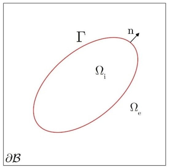
Figure 3.
Rectangular box with and .
Here and are the differential operators of PDEs in and .
Regarding the single interface problem (10)–(13), Green’s functions associated with two partial differential equations are in general not identical. is considered as the Green’s function corresponding to PDE (10) defined in the interior domain and satisfies
is the Green’s function corresponding to (11) in the exterior domain and satisfies
Using density function , double layer boundary integrals are written as
Using density function , single layer boundary integrals are written as
The interior and exterior volume integrals are written as
Besides, the operator of adjoint double layer and hyper-singular single layer boundary integrals are , , and , respectively, defined as
The solution to the single interface problem is then defined as
Two boundary integral equations are derived from by interface condition (15)
The integral equations shown above can be written in matrix form
Generally, the analytic expression of Green’s function is typically impossible to derive for PDEs defined in complex geometry with variable coefficients and it is hard to derive even if it is available in some cases, as mentioned before. Instead of direct calculation of boundary integrals, the KFBIM evaluates volume and boundary integrals as a result of solving an equivalent interface problem which is an interpolation of values on a Cartesian grid. To solve the newly defined equivalent interface problems, first, the interface problem is discretized using a finite difference scheme; second, the numerical corrections are made at irregular points in the discrete system to ensure the second order accuracy; third, fast PDE solvers are utilized to solve the equivalent interface problems, for example, the geometric multigrid preconditioned conjugate gradient iterative method (GMG-PCG); lastly, the boundary integral values are interpolated by the Birkhoff interpolation on the interface. Using a Generalized Minimal Residual (GMRES), the resultant linear system is solved iteratively [31,32]. Details such as discretization of PDE, corrections for the discrete system, solutions and fast solvers of the discretized system of finite difference equations, and interpolation method of volume and boundary integrals on the boundary are presented in [16,17,18,19,20,21,22].
4. Boundary Reconstruction and Implementation of the Kernel Free Boundary Integral Method
This section presents the proposed boundary reconstruction approach and the implementation of the KFBIM for magnetostatics analysis. To do the geometry reconstruction and analyze the problem of C-core, first, since the KFBIM is not dimensional, the de-unitization of the problem must be performed. The chosen characteristic length is 10cm. After de-unitization, the rectangle air box becomes , which is the size of the outer box by default in the algorithm. For the original C-core boundary with sharp corners, the inner radius and the outer radius are 0.45 and 0.65, respectively. The centers of the two coils are located at (−0.27, 0) and (−0.83, 0) with a radius of 0.14.
4.1. Boundary Reconstruction
To reconstruct the boundary, the zero-padded/filled inverse discrete Fourier transform (inverse DFT) is adopted. The first step is to perform the discrete Fourier transform (DFT) on the boundary. Since this problem is 2D based, the boundary can be represented on the complex plane as , . However, it is easier to use simple coordinate pairs of real numbers , , in real space, to get two Fourier Series for two real functions since they have the same period and they are synchronized together by definition. Additionally, the DFT of both and are
To fill the zeros in the data sets, the Fourier Transforms are rearranged by shifting the zero-frequency-component to the center of data set, so for the odd number , the sequence becomes , and for the even number , . For the odd number , the zero-padded data is defined as
For even number , the zero-padded data defined as
Then, the data is reconstructed by filling with zeros up to the size of and applying the inverse DFT for the zero-padded data sets.
The original and reconstructed boundaries are shown in Figure 4 and Figure 5. The curve is smoothed by the zero-padded inverse DFT method, so theoretically, the problem can be solved accurately. The example shown is the boundary for the grid of 256 × 256, the number of points is filled from 288 to 440, and 440 is the boundary number suitable for a 256 × 256 grid calculated based on the arc length to make sure there is only one point in one element of the mesh grid.
where is the length of each element meshed by the finite difference mesh methods.
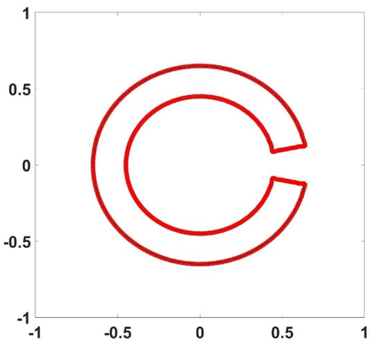
Figure 4.
The reconstructed boundary and original geometry.
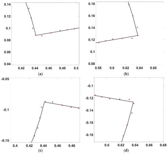
Figure 5.
The zoomed-in images of the reconstructed boundary and original boundary near the sharp corners: (a) upper left corner; (b) upper right corner; (c) lower left corner; (d) lower right corner.
4.2. Implementation of KFBIM
In , the material is air or vacuum, and the material in is iron. Following the formulation of KFBIM derived in Section 3, the single boundary magnetostatic problem in 2D is defined as
The permeability in is set to be , which is the permeability of air or vacuum. In this study, there are two cases for the permeability of iron : for one of two settings, the relative permeability of the material of the C-core is spatially constant at 1000; for the other setting, an inhomogeneous permeable material is used to represent the iron and the relative permeability of the iron of the C-core is set to .
In the electromagnetic package of commercially available FEM, for example, ANSYS Maxwell, the constant current of 100 A or current density 162,403 A/m2 is set for the coils (1000 and 16,240.3 after de-unitization) for this problem. For KFBIM, is 0 in because there are no current flows in the C-core, and for the current flow through the coils, a smooth modified Sigmoid function is selected to model distributed current source. The smooth modified Sigmoid function is defined as
Note that the integral of the first portion and second portion of Sigmoid functions shown above in the domain box are both 1000, which is the same value of the de-unitization of 100A, but the center of two portions are different and located at the center of the two coils, and the 3D shape of two portions are very similar to shapes of two coils of the C-core magnetostatics problem.
5. Results and Discussion of KFBIM
5.1. Numerical Example
Before comparing the results of the smoothed C-core, computed by KFBIM and the results of the original C-core calculated by FEM, there is a general numerical test to show how much accuracy can be improved by the smoothed C-core for the KFBIM to overcome the singularity problem on the sharp corner. The examples are solved on the 256 × 256 grid. In [26], it has been found that problems converge when KFBIM solves them on the 256 × 256 grid, and a more convergent study of the boundary integral method can be found in [11]. In addition, using the 256 × 256 grid, the KFBIM is more computationally efficient than FEM (ANSYS). The boundary conditions for the following examples can be found in the equations in Section 2.2.
Example: In this example, we consider an interface problem as follows
with the KFBIM for the problem with the boundary before and after the reconstruction. For the interface problem, the sources and , and the interface conditions and are selected so that the solution reads exactly
The errors are shown in Table 3.
Table 3.
Errors of the original boundary and the reconstructed boundary.
As shown in the Table, the numerical errors are reduced significantly on the smoothed boundary. The error can be improved around three times, and the max error can be improved by around five times.
5.2. Comparison between KFBIM and FEM on Magnetostatic Analysis
The field computation results from KFBIM are compared with FEM and discussed in this section. The FEM computations are delivered using a commercial FEM package for electromagnetics problems; ANSYS Electronics, which is a popular numerical field analysis tool. In the software, the Maxwell 2D package is used to solve 2D electromagnetics problems. The simulations are processed using an Intel(R) Core (TM) i7-8750H CPU @ 2.20 GHz.
Example 1: spatially constant permeable material.
First, the comparison of flux density magnitude is conducted point-by-point. For KFBIM, a 256 × 256 grid is used to analyze the C-core magnetostatics problem. The problem is analyzed by FEM using the mesh of 268,535 elements since the study [26] shows the accuracy level of KFBIM on the 256 × 256 grid is the same as FEM using a mesh of 268,535 elements. Figure 6 shows the field density results analyzed for each point on the 256 × 256 grid by FEM and KFBIM. Figure 7 shows the comparison of flux densities in 3D.
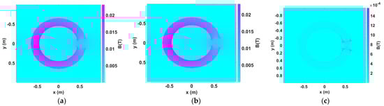
Figure 6.
Flux density results comparison between KFBIM for the reconstructed boundary and FEM for the original boundary for Example 1: (a) Flux density (T) of the reconstructed C-core problem (KFBIM) (256 × 256); (b) Flux density (T) of the original C-core problem (FEM) (268,535 elements); (c) Difference of flux density (T) between FEM and KFBIM.
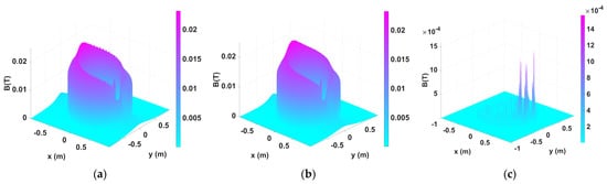
Figure 7.
Flux density results comparison between KFBIM for the reconstructed boundary and FEM for the original boundary in 3D for Example 1: (a) Flux density (T) of the reconstructed C-core problem (KFBIM) (256 × 256); (b) Flux density (T) of the original C-core problem (FEM) (268,535 elements); (c) Difference of flux density (T) between FEM and KFBIM.
Based on the difference between the results of FEM and KFBIM, there is some degree of differences in the reconstructed boundary, especially on the corners. The reason why some differences exist is after the reconstruction, the corner of boundary is smoothed and not the same as the original boundary. However, from the figure, we can see that the difference is not high, and the peak value around the corner is almost the same. Additionally, the normalized RMS difference is very low. The normalized RMS difference (NRMS) is computed by:
which is 0.7%. In addition, the inductance is also compared between KFBIM and FEM. The inductance calculated by FEM is 3.76439 × 10⁻⁶ and 3.7592 × 10⁻⁶ is calculated by KFBIM. The difference is 0.13% of the FEM results. If this method is extended to the area of the electrical machine, the field at the airgap is more important, because the magnetic forces are calculated by the flux density on the airgap. The difference in airgap is very small. The computational time of FEM and KFBIM is 117.84 s and 4.67 s, respectively.
Example 2: inhomogeneous permeable (spatially variable permeability) material.
The relative permeability in this example of the C-core material is: , which is the spatial variable mentioned in Section 4. For this example, the comparisons of the results include inductance and flux density, which is similar to the first example. The field density results analyzed for each point on the 256 × 256 grid by FEM and KFBIM are shown in Figure 8. In addition, Figure 9 shows the flux densities comparison in 3D.
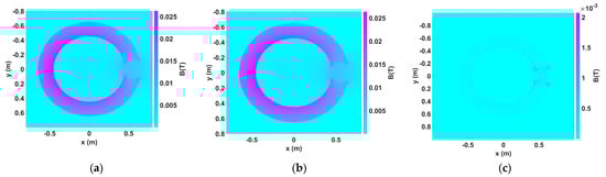
Figure 8.
Flux density results comparison between KFBIM for the reconstructed boundary and FEM for the original boundary for Example 2: (a) Flux density (T) of the reconstructed C-core problem (KFBIM) (256 × 256); (b) Flux density (T) of the original C-core problem (FEM) (268,535 elements); (c) Difference of flux density (T) between FEM and KFBIM.
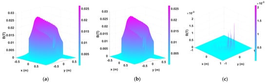
Figure 9.
Flux density results comparison between KFBIM for the reconstructed boundary and FEM for the original boundary in 3D for Example 2: (a) Flux density (T) of the reconstructed C-core problem (KFBIM) (256 × 256); (b) Flux density (T) of the original C-core problem (FEM) (268,535 elements); (c) Difference of flux density (T) between FEM and KFBIM.
The difference in the corner is almost the same as Example 1. The normalized RMS difference is computed to be 0.602%. The inductance calculated by FEM is 3.8510 × 10⁻⁶ , and 3.8696 × 10⁻⁶ is calculated by KFBIM. The computational time of FEM and KFBIM is 133.78 s and 5.07 s, respectively. Although the Gibbs phenomenon is not obvious in this case, for some cases, it may need to be taken into account using some special methods [18]. The Gibbs ringing artifact appears because a discontinuity cannot be represented by the Fourier series with a finite number of harmonics. Therefore, the discontinuity leads to a decaying, oscillating spectrum.
This study shows that the proposed sharp corner reconstruction method works for the magnetostatics analysis of C-core, which could be used for the inductor design. For the general numerical example, using the reconstructed method, the error and the max error can be improved by several times. Not only can the constant permeability material problem be solved by KFBIM as shown in Example 1, but Example 2 also shows the nonhomogeneous permeable material problem can be solved by KFBIM, which is one of the advantages of KFBIM as well compared to other traditional boundary integral methods. Although the impact of the material with the B-H curve is not considered in this study, it will be incorporated in a future study with some additional techniques such as spline interpolation or other proper iterative methods. While the three-dimensional application is not the current focus of this paper, KFBIM in three-dimensions has been developed in this paper [31]. However, the interface problem solver in three-dimensions is still underdeveloped. Therefore, after the 3D interface problem solver is finished, it could be applied to magnetostatics analysis with the proposed boundary reconstruction method. Although the numerical results are not compared with actual C-core behaviors, experimental studies will be conducted on the development of the KFBIM and after finishing an optimization scheme.
6. Conclusions
This paper introduces a new approach to deal with sharp corners in the kernel-free boundary integral method. It investigates the effectiveness of a sharp corner reconstruction method in solving two-dimensional magnetic field problems, specifically those involving geometries with sharp corners. The study utilizes a boundary reconstruction method based on the discrete Fourier transform (DFT) and inverse DFT to smoothen the sharp corners. The kernel-free boundary integral method (KFBIM) is then employed to analyze a 2D electromagnetics problem involving a toroidal core with an airgap and sharp corners. The numerical example demonstrates the effectiveness of the boundary reconstruction technique. Additionally, the paper compares the flux density, inductance, and computational time results obtained from KFBIM with those from the finite element method (FEM) software (ANSYS) applied to the original geometry.
The findings indicate that while there may be slight differences in flux density at the corners, the overall discrepancy and the variation in inductance are minimal. This suggests that the boundary reconstruction method provides a relatively high level of accuracy for magnetostatic analysis. The combination of a smoothed boundary through reconstruction and the computational efficiency of KFBIM is crucial for optimizing electromagnetic designs, even in complex geometries with sharp corners. As a result, KFBIM emerges as a reliable alternative method, along with the sharp corner reconstruction approach, for analyzing electromagnetics problems, particularly in the design of devices such as inductors and transformers. It can potentially serve as a valuable analysis and design tool for engineers in this field.
Author Contributions
Conceptualization, Z.J. and M.K.; methodology, Z.J., S.L. and W.Y.; software, Z.J., Y.C. and W.Y.; validation, Z.J.; formal analysis, Z.J.; investigation, Z.J. and M.K. and S.L.; resources, M.K.; data curation, Z.J.; writing—original draft preparation, Z.J.; writing—review and editing, Z.J. and M.K., W.Y. and S.L.; visualization, Z.J.; supervision, M.K. and S.L.; project administration, M.K.; funding acquisition, M.K. All authors have read and agreed to the published version of the manuscript.
Funding
This research was funded by the National Science Foundation, Division of Electrical, Communications and Cyber Systems grant ECCS-1927432. Shuwang Li was partially funded by the National Science Foundation, Division of Mathematical Sciences grant DMS-1720420 and DMS-2309798.
Data Availability Statement
The data presented in this study are available on request from the author panel.
Conflicts of Interest
The authors declare no conflict of interest.
References
- Yang, Z.; Shang, F.; Brown, I.P.; Krishnamurthy, M. Comparative Study of Interior Permanent Magnet, Induction, and Switched Reluctance Motor Drives for EV and HEV Applications. IEEE Trans. Transp. Electrif. 2015, 1, 245–254. [Google Scholar] [CrossRef]
- Salameh, M.; Brown, I.P.; Krishnamurthy, M. Fundamental Evaluation of Data Clustering Approaches for Driving Cycle-Based Machine Design Optimization. IEEE Trans. Transp. Electrif. 2019, 5, 1395–1405. [Google Scholar] [CrossRef]
- Salameh, M.; Singh, S.; Li, S.; Krishnamurthy, M. Surrogate Vibration Modeling Approach for Design Optimization of Electric Machines. IEEE Trans. Transp. Electrif. 2020, 6, 1126–1133. [Google Scholar] [CrossRef]
- COMSOL, AC/DC Module. Available online: https://www.comsol.com/acdc-module (accessed on 15 April 2023).
- ANSYS, Inc., ANSYS Maxwell. Available online: https://www.ansys.com/products/electronics/ansys-maxwell (accessed on 15 April 2023).
- Peng, J.; Salon, S.; Chari, M. A comparison of finite element and boundary element formulations for three-dimensional magnetostatic problems. IEEE Trans. Magn. 1984, 20, 1950–1952. [Google Scholar] [CrossRef]
- Normann, N.; Borgermann, F.; Mende, H. Simple boundary element method for three-dimensional magnetostatic problems. IEEE Trans. Magn. 1985, 21, 1235–1239. [Google Scholar] [CrossRef]
- Salon, S. The hybrid finite element-boundary element method in electromagnetics. IEEE Trans. Magn. 1985, 21, 1829–1834. [Google Scholar] [CrossRef]
- Li, S.; Lowengrub, J.; Leo, P. A rescaling scheme with application to the long-time simulation of viscous fingering in a Hele-Shaw cell. J. Comput. Phys. 2007, 225, 554–567. [Google Scholar] [CrossRef]
- Li, S.; Li, X. A Boundary Integral Method for Computing the Dynamics of an Epitaxial Island. SIAM J. Sci. Comput. 2011, 33, 3282–3302. [Google Scholar] [CrossRef]
- Hao, W.; Hu, B.; Li, S.; Song, L. Convergence of boundary integral method for a free boundary system. J. Comput. Appl. Math. 2008, 334, 128–157. [Google Scholar] [CrossRef]
- Brovont, A.D. Exploring the boundary element method for optimization-based machine design. In Proceedings of the 2017 IEEE International Electric Machines and Drives Conference (IEMDC), Miami, FL, USA, 21–24 May 2017; pp. 1–7. [Google Scholar] [CrossRef]
- Howard, R.; Brovont, A.; Pekarek, S. Analytical Evaluation of 2-D Flux Integral for Magnetostatic Galerkin Method of Moments. IEEE Trans. Magn. 2016, 52, 1–8. [Google Scholar] [CrossRef]
- Araujo, D.M.; Coulomb, J.-L.; Chadebec, O.; Rondot, L. A Hybrid Boundary Element Method-Reluctance Network Method for Open Boundary 3-D Nonlinear Problems. IEEE Trans. Magn. 2014, 50, 77–80. [Google Scholar] [CrossRef]
- Jin, Z.; Cao, Y.; Li, S.; Ying, W.; Krishnamurthy, M. A Kernel-Free Boundary Integral Method for 2-D Magnetostatics Analysis. IEEE Trans. Magn. 2023, 59, 1–19. [Google Scholar] [CrossRef]
- Ying, W.; Wang, W.-C. Kernel-Free Boundary Integral Method for Variable Coefficients Elliptic PDEs. Commun. Comput. Phys. 2014, 15, 1108–1140. [Google Scholar] [CrossRef]
- Ying, W.; Henriquez, C.S. kernel-free boundary integral method for elliptic boundary value problems. J. Comput. Phys. 2007, 227, 1046–1074. [Google Scholar] [CrossRef]
- Xie, Y.; Ying, W. Fourth-Order Kernel-Free Boundary Integral Method for the Modified Helmholtz Equation. J. Sci. Comput. 2018, 78, 1632–1658. [Google Scholar] [CrossRef]
- Xie, Y.; Ying, W. A fourth-order kernel-free boundary integral method for implicitly defined surfaces in three space dimensions. J. Comput. Phys. 2020, 415, 109526. [Google Scholar] [CrossRef]
- Xie, Y.; Ying, W.; Wang, W.-C. High-Order Kernel-Free Boundary Integral Method for the Biharmonic Equation on Irregular Domains. J. Sci. Comput. 2019, 80, 1681–1699. [Google Scholar] [CrossRef]
- Cao, Y.; Xie, Y.; Krishnamurthy, M.; Li, S.; Ying, W. A kernel-free boundary integral method for elliptic PDEs on a doubly-connected domain. J. Eng. Math. 2022, 136, 2–22. [Google Scholar] [CrossRef]
- Ying, W.; Wang, W.-C. kernel-free boundary integral method for implicitly defined surfaces. J. Comput. Phys. 2013, 252, 606–624. [Google Scholar] [CrossRef]
- Brovont, A.D. A Galerkin Boundary Element Method for Two-Dimensional Nonlinear Magnetostatics. Ph.D. Dissertation, Purdue University, West Lafayette, IN, USA, 2016. [Google Scholar]
- Paris, F.; Canas, J. Boundary Element Method-Fundamentals and Applications; Oxford University Press: Oxford, UK, 1997. [Google Scholar]
- Amartur, S.; Haacke, E.M. Modified iterative model based on data extrapolation method to reduce Gibbs ringing. J. Magn. Reson. Imaging 1991, 1, 307–317. [Google Scholar] [CrossRef] [PubMed]
- Constable, R.T.; Henkelman, R.M. Data extrapolation for truncation artifact removal. Magn. Reson. Med. 1989, 17, 108–118. [Google Scholar] [CrossRef] [PubMed]
- Martin, J.F.; Tirendi, C.F. Modified linear prediction modeling in magnetic resonance imaging. J. Magn. Reson. 1989, 82, 392–399. [Google Scholar] [CrossRef]
- Eroglu, A. Complete Modeling of Toroidal Inductors for High Power RF Applications. IEEE Trans. Magn. 2012, 48, 4526–4529. [Google Scholar] [CrossRef]
- Lopez-Villegas, J.M.; Vidal, N.; del Alamo, J.A. Optimized Toroidal Inductors Versus Planar Spiral Inductors in Multilayered Technologies. IEEE Trans. Microw. Theory Tech. 2017, 65, 423–431. [Google Scholar] [CrossRef]
- Thotabaddadurage, S.U.S.; Kularatna, N.; Steyn-Ross, D.A. Optimization of Supercapacitor Assisted Surge Absorber (SCASA) Technique: A New Approach to Improve Surge Endurance Using Air-Gapped Ferrite Cores. Energies 2021, 14, 4337. [Google Scholar] [CrossRef]
- Saad, Y.; Schultz, M.H. GMRES: A Generalized Minimal Residual Algorithm for Solving Nonsymmetric Linear Systems. SIAM J. Sci. Stat. Comput. 1986, 7, 856–869. [Google Scholar] [CrossRef]
- Saad, Y. Iterative Methods for Sparse Linear Systems; PWS Publishing Company: Boston, MA, USA, 1996. [Google Scholar]


Disclaimer/Publisher’s Note: The statements, opinions and data contained in all publications are solely those of the individual author(s) and contributor(s) and not of MDPI and/or the editor(s). MDPI and/or the editor(s) disclaim responsibility for any injury to people or property resulting from any ideas, methods, instructions or products referred to in the content. |
© 2023 by the authors. Licensee MDPI, Basel, Switzerland. This article is an open access article distributed under the terms and conditions of the Creative Commons Attribution (CC BY) license (https://creativecommons.org/licenses/by/4.0/).