Article

Opportunities to Improve Marine Power Cable Ratings with Ocean Bottom Temperature Models

1
School of Ocean and Earth Science, National Oceanography Centre, University of Southampton, Southampton SO14 3ZH, UK
2
Tony Davies High Voltage Laboratory, School of Electronics and Computer Science, University of Southampton, Southampton SO17 1BJ, UK
3
Ocean Infinity, Unit 1 Keel Rd., Woolston, Southampton SO19 9UY, UK
*
Author to whom correspondence should be addressed.
Energies 2023, 16(14), 5454; https://doi.org/10.3390/en16145454
Submission received: 24 May 2023 / Revised: 7 July 2023 / Accepted: 12 July 2023 / Published: 18 July 2023
(This article belongs to the Section F: Electrical Engineering)

Abstract

:
Determining reliable cable ampacities for marine High Voltage Cables is currently the subject of significant industry and academic reassessment in order to optimize (maximizing load while maintaining safe operating temperatures) design and reduce costs. Ampacity models can be elaborate, and inaccuracies are increasingly predicated on the uncertainty in environmental inputs. A stark example is the role of ambient temperature at cable depth, which, due to the scale of cables and the inaccessibility of the seafloor, is commonly estimated at 15 °C. Oceanographic models incorporating ocean bottom temperature are increasingly available, and they achieve coverage and spatiotemporal resolutions for cable applications without the requirement for project specific measurements. Here, a rudimental validation of the AMM15 and AMM7 mean monthly ocean bottom temperature models for the NW European Shelf indicates encouraging accuracies (MBE ≤ 1.48 °C; RMSE ≤ 2.2 °C). A series of cable case studies are used to demonstrate that cable ratings can change between −4.1% and +7.8% relative to ratings based on a common static (15 °C) ambient temperature value. Consideration of such variations can result in both significant ratings (and hence capital expenditure and operating costs) gains and/or the avoidance of cable overheating. Consequently, validated modelled ocean bottom temperatures are deemed sufficiently accurate, providing incomparable coverage and spatiotemporal resolutions of the whole annual temperature signal, thereby facilitating much more robust ambient temperatures and drastically improving ampacity estimates.

1. Introduction

1.1. Significance of Marine Power Cables

The global energy network is increasingly reliant on marine High Voltage (HV) power cables, either transmitting power across shelf seas from offshore renewables (e.g., wind) or trading energy between countries [1,2]. In 2021, the UK’s offshore wind capacity increased to 11.3 GW, second only to China (24.5 GW) globally, providing 11% (36.6 TWh) of the UK’s total power generation, which was enough for ~33% of UK homes, and saving an estimated 14 Million tonnes of CO2 [3,4]. Similarly, the UK’s interconnector capacity increased to 7.4 GW, facilitating a net import of 24.6 TWh (7.4% of total supply) from predominantly French (52.7%) but also Belgian (24.3%), Dutch (15.1%), Norwegian (4.8%), and Irish (3.0%) power [3]. Furthermore, to meet future energy demands and net zero carbon emissions, the UK plans to achieve 50 GW offshore wind [5] and 18 GW interconnector capacity [5] by 2050, driving significant expansion of marine HV cables predominantly through the shallow (<200 m) North West European Shelf [6]. Similar expansion is now occurring on a global basis. Consequently, recent research is increasingly focused on maintaining safe and efficient marine cable operations, optimizing capital expenditure (CAPEX), and lowering the levelized cost of electricity, all of which are growing concerns for national energy security and fundamental to capitalizing on the growing offshore renewable and evolving energy markets [2].

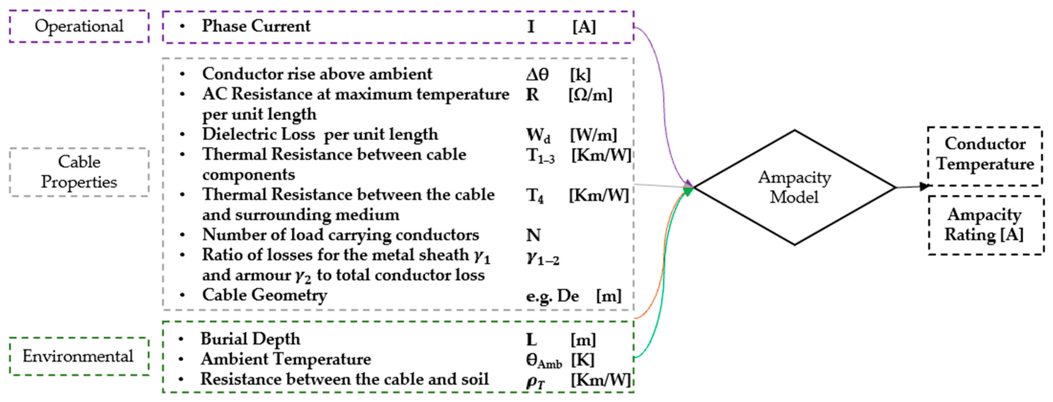
1.2. Cable Ampacity Evaluation Environmental Inputs and Shortcomings

A primary concern of HV cable design is reliably resolving the ampacity “rating” or maximum safe operating current using ampacity models (e.g., IEC-60287) [7]) that incorporate both properties of the cable as well as operational and environmental factors (e.g., Figure 1). The rating limits the cable to safe operating temperatures of 90 °C for AC [8] or 70 °C for DC [9] cables. This, in turn, informs the choice of the cable cross sectional area, which significantly impacts the capital expenditure and/or informs remediation, such as the thermal optimization of trench back-fill. Ampacity models (e.g., IEC-60287) have a sound theoretical basis and proven utility [10,11], and they are increasingly computationally advanced. Bespoke finite element models (FEM) are also utilized to resolve more realistic 2D complex (in-homogeneous) backfill environments with heterogeneous thermal properties [10,11,12,13,14,15] with coupled conductive-convective components [15,16,17,18] at varying computational cost [16].
While ampacity models advance, their accuracy and reliability have been increasingly shown to be predicated on the quality of their environmental inputs (e.g., [1,16]), but they have received considerably less attention during the process of actual cable design. The implications of the thermal resistivity of the burial environment has been the focus of research (e.g., [16,17,18,19]), whilst the implications of the post-installation of depth of cover changes through seabed movement has long been established, although it is difficult to predict over the lifetime of any cable design [9]. By contrast, the impacts of spatial and temporal variation in ambient temperature at cable depth on cable rating has only recently been addressed [19]. Recent studies of Distributed Temperature Sensor data from active cables shows how strongly cable temperature can be controlled by ambient temperature variations [20,21].
For submerged marine HV cables, ambient temperature at cable depth is controlled by the ambient ocean bottom temperature (OBT), which is then attenuated at a rate determined by the thermal diffusivity of the soil as it propagates to the depth of lay (typically 1–3 m) [8,22]. The spatial and temporal variation of OBT can be large as it is controlled by a wide range of oceanographic factors, including water depth, tidal mixing, density-driven currents, and seasonal variations in both wind forcing and solar irradiation [23]. The scale of these variations are such that cables can experience both significant seasonal and, as cable lengths increase (e.g., >80 km AC [24], >300 km DC) [25]), spatial variations. Despite these potential changes, standard cable design practice routinely considers 10 °C, 12 °C, or, most commonly, 15 °C to be a representative estimate of ambient temperature at cable depth, irrespective of the location of the cable or how it will be operated over a year [26,27]. A rare example of considering proximal ocean bottom temperature measurements [14] demonstrated that the standard assumption was 10 °C lower than that of the summer OBTs, resulting in potentially dangerous cable-operating temperatures.

1.3. Ocean Bottom Temperature Models

The scale of cables and the inaccessibility of the ocean floor makes resolving representative ambient OBT difficult, and a bespoke campaign of measurement for individual cables would be impractical. Publicly available proximal observations are available, but these almost never resolve the full annual signal that is required for comprehensive analysis [22]. Fortunately, oceanographic models incorporating ambient OBT are increasingly available for large parts of the globe. For the Northwest European Shelf, two such models include the Atlantic Margin Models AMM7 and the AMM15, which are both available from the Copernicus Marine Environment Monitoring Service (CMEMS) (see Figure 2a).
Due to the paucity of in situ time-series measurements of OBT across the domain (only five locations in total), calibration of these modelled values is relatively restricted [28,29,30]. Although these deployments have high temporal resolutions (hours/days), they tend to cover only short periods (a few months). Similarly, to date, validation has been against an EN4 database that provides overall mean bias errors for water depths < 500 m of 0.37 ± 1.0 °C for AMM15 and of 0.47 ± 1.12 °C for AMM7 [30].
Due to the filtering effect of the seabed, short-term (hours/days) temperature fluctuations are not propagated to cable depth [20]. The temporal lag of this propagation will depend on a combination of the depth of the burial of the cable as well as the thermal diffusivity of the burial environment. With typical marine sediments having thermal diffusivities of between 3 and 7 × 10⁻⁷ m2s−1 and burial depths of 1–3 m, this equates to temperatures having to persist in the water column for 2–5 weeks typically in order to generate significant temperature changes at actual cable depth. Therefore, for consideration in cable design, mean monthly modelled ocean bottom temperatures are considered the most appropriate parameter to have validated. Although summer seasonal variations have previously been calculated [30], the accuracy and the precision of mean monthly values, which are essential for cable modelling purposes, are not available.

1.4. Paper Aims

  • To devise a transparent method for improving the validation and utilization of publicly accessible OBT models for cable design using the Northwest European shelf AMM7 and AMM15 as exemplars (Section 3).
  • To demonstrate the spatial and temporal variation in mean monthly modelled OBTs along “indicative” cable routes across the Northwest European Shelf (Section 4).
  • To demonstrate the impact of applying these temporally varying OBT model outputs to IEC-based cable rating algorithms to cable conductor temperature and overall rating (Section 5).

2. Materials

2.1. Ocean Bottom Temperture Models

The detailed description of the AMM7 and AM15 models used in this study are summarized in [28,29,30]. Both models are based on Forecast Ocean Assimilation Models (FOAM) [29], which, in turn, combines the Nucleus for European Modelling of the Ocean model (NEMO) forced by lateral boundary conditions from the UK Met Office North Atlantic Ocean forecast model. Atmospheric forcing is given by the operational European Centre for the Medium-Range Weather Forecasts (ECMWF) numerical weather prediction model for the AMM15 and by the operational UK Met Office Global Atmospheric Model for AMM7.
The AMM7 model has a resolution of 7 km whilst the (finer) AMM15 model has a resolution of 1.5 km, which better defines coastlines as well as dynamic features, such as coastal currents, oceanic fronts, and mesoscale eddies, which vary in size from a few kilometers on shelf seas to tens of kilometers in deeper waters [29,30]. The AMM15 model also uses a more detailed bathymetry, i.e., EMODnet 2015, rather than the coarser GEBCO bathymetry that is used by AMM7. The AMM7 model thus misses some finer oceanographic features as well as poorly representing depth variation in some of the on-shelf regions of the North Sea [30].
Both the AMM15 and the AMM7 models provide hourly and daily predictions of sea surface and ocean bottom temperature, salinity, horizontal currents, sea level height, and mixed layer depth. For this study, the daily mean OBT modelled output was used to produce the mean and standard deviations for each month. The resulting monthly OBT end members (January and August) are visualized in Figure 3. Based on the availability of the available data, the models were averaged over the following periods: 1 January 2019–17 January 2022 for AAM15, and 1 May 2019–17 January 2022 for AMM7.

2.2. In Situ Measured Ocean Bottom Temperature Dataset Construction

The World Ocean Database (WOD) is considered the largest and simplest database of oceanographic data [31], from which other frequently quoted but variably processed databases (e.g., EN4 [32], CEFAS [33], and IQuOD [31]) are derived. Oceanographic variables, including OBT, are readily accessible (for this paper, accessed 17 January 2022, following [34]). A pre-quality controlled (Section 3) dataset was constructed that enabled the following:
  • It restricted the search area to within the AMM15 and AMM7 model domains Figure 2 and Figure 3.
  • It removed erroneous entries, e.g., corrupted files, deployments with missing measurements, and files with corrupted metadata.
  • It retained only those measurements within +/− 5m of the EmodNET bathymetry at each location.

3. Quality Control of In Situ Observations and Validation Methodology

Recent studies on the uncertainties associated with the measurement of a range of oceanographic parameters have identified that a number of instrument types, e.g., Expendable [XBT] or Mechanical BathyThermographs [MBT]), have uncertainties one to two orders of magnitude greater than other forms of instrumentation [31,35]. Rather than just removing whole sets of instrumentation, a transparent quality control step is used to identify extreme bias (modelled minus measured) errors relative to their monthly bias error distributions. It is recognised that removing values that disagree with the model could bias a validation in favor of the model, and thus requires evaluation. However, the number of extreme anomalies should, by definition, be proportionally insignificant. Consequently, the post-quality control distribution should visibly improve while minimizing the impact on the validation statistics.

3.1. Quality Controlled (QC) In Situ Database

For each observation, the bias error and the square error are calculated comparing the mean monthly modelled OBTs to observations:
  • Bias Error:
    BE = modelled OBT − measured OBT
  • Square error:
    SE = (modelled OBT − measured OBT)2
Both (BE) and (SE) comprise the measured error and modelled error, but only BE maintains the sign, preserving whether the model is anomalously hot (positive) or cold (negative). To transparently identify potential anomalies, a simple “fast” statistical extreme anomaly filter (e.g., [36]) was applied. For each month, the extreme anomalies were identified as those with bias errors exceeding the monthly distributions bound by the equations below:
  • Extreme positive anomalies > 3rd BE quartile + 3 × BE interquartile range.
  • Extreme negative anomalies < 1st BE quartile − 3 × BE interquartile range.
An upper and lower extreme anomaly limit is calculated using both models and is then combined, ensuring the post-quality controlled measured dataset contains no ex treme anomalies from the perspective of either models (see Figure 4).

3.2. Validation Methodology

For each observation and each monthly mean, the following model validation summary statistics are tabulated in order to evaluate model accuracy pre- and post-QC:
  • Mean Bias Error: MBE = B E ¯ (MBE ± σBE is reported).
  • Mean Absolute Error: MAE = B E ¯ (MAE ± σMAE is reported).
  • Bias Error Standard Deviation:
    σ B E = ( B E B E ) ¯ n 1
  • Root Mean Square Error:
    RMSE = S E

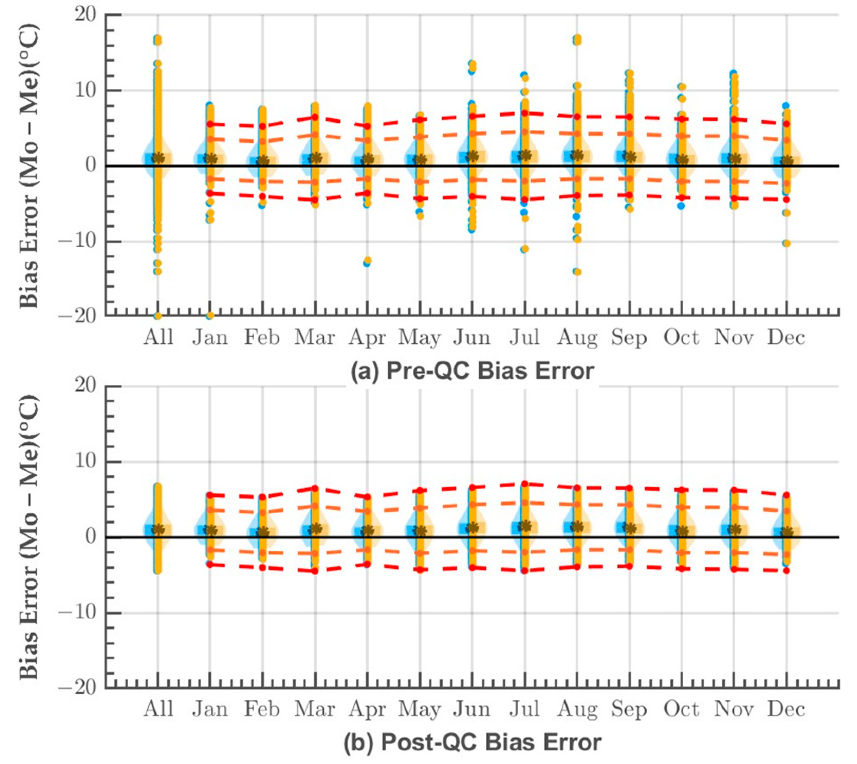
3.3. Quality Control and Validation Results

The pre-quality-controlled database contained 182,637 observations (Figure 4a and Table 1), with the least observations in December (7507) and the most in August (20,589). Bias error distribution demonstrates anomalous observations distinct from the main distributions, which are isolated by the extreme anomaly filter.
The post-quality control dataset has 777 extreme anomalies removed, leaving 181,860 observations remaining, with the least in December (7496) and the most in August (20,480). The effect of the quality control filter varied, improving 8/12 (AMM7) and 6/12 (AMM15) monthly MBEs and 11/12 (AMM7), 7/12 (AMM15) monthly RMSEs. While the magnitude of anomalous bias errors in the pre-QC dataset can be large (>10 °C), their numbers are actually few. Consequently, the impact of quality control on validation statistics is minimal, with the MBE for the whole dataset changing by only −0.05 °C for AMM7 and +0.01 °C for AMM15. The RMSE improved for both datasets by 0.08 °C (AMM7) and 0.03 °C (AMM15). The consequence of quality control on monthly validation statistics ranged by, at most, MBE = 0.17 °C (AMM15 March), MBE = −0.22 °C (AMM15 September) and RMSE = 0.11 °C (AMM15 June and July), and RMSE = −0.11 °C (AMM7 August). As such, the extreme anomaly filter is considered to be very effective at removing visibly dubious anomalies, thereby improving the bias error distribution (see Figure 4) without impacting the validation statistics.
The post-quality controlled (Post-QC) datasets are heavily dominated by measurements from fixed ocean station data and CTD profilers (Figure 5), with other instrumentation representing only 18.6% of the data. There is excellent spatial coverage across the case-study domain (Figure 6), and all months bar December have >10,000 measurements for comparison (December has ~7500).

3.4. Validation Intepretation

The (Post-QC) validation demonstrates that both models perform well, with the AMM7 model performing marginally better than the AMM15 (Table 1). The whole domain, annual RMSEs range was between 1.64 °C (AMM7) and 1.67 °C (AMM15). The whole domain, monthly RMSEs range was between 1.28 °C (February) and 2.07 °C (July) for the AMM7 model and 1.28 °C (February) to 2.2 °C (July) for the AMM15 model. Bias error distributions (Figure 4) clearly demonstrate how similarly the models performed, with whole domain, annual net positive MBEs of +1.03 °C (AMM7) and +1.06 °C (AMM15). The whole domain, monthly MBE ranges were between 0.61 °C (February) and 1.38 °C (August) for the AMM7 model and 0.67 °C (February& December) and 1.48 °C (August) for the AMM15 one. Both models demonstrate that their performance is temporally variable––i.e., significantly better in the winter months (Oct–May: 1.09 °C ≥ MBE ≥ 0.61 °C; 1.66 °C ≥ RMSE ≥ 1.38 °C) than in the summer months (Jun–Sep: 1.48 °C ≥ MBE ≥ 1.17; 2.2 °C ≥ RMSE ≥ 1.69 °C).
The geographical distribution of these bias errors (Figure 7) demonstrates that model performance is also spatially variable, with the greatest positive bias errors clustered in the East Central North Sea and German Bight regions in the summer months. By contrast, the lowest bias error cluster, including some negative ones, is in the winter months, particularly along the outer shelf margins and in the Norwegian trench regions, and these observations are supported by previous assessments of temporally restricted assessments [31]. The dominant positive bias of the models (i.e., they are predicting marginally higher temperatures than have actually been observed) is regarded as a positive for cable modelling because it ensures a degree of conservatism. Conversely, net cold biases are restricted to shelf-break and off-shelf regions that are far from the major expansions of the cable routes (Figure 7).
Ultimately, the validation demonstrates that both models perform similarly with whole-shelf and whole-year statistics of 1.25 ± 1.06 °C (@ 1 STDEV) MAE for the AMM7 model and 1.27 ± 1.08 °C (@ 1 STDEV) MAE for the AMM15 model.

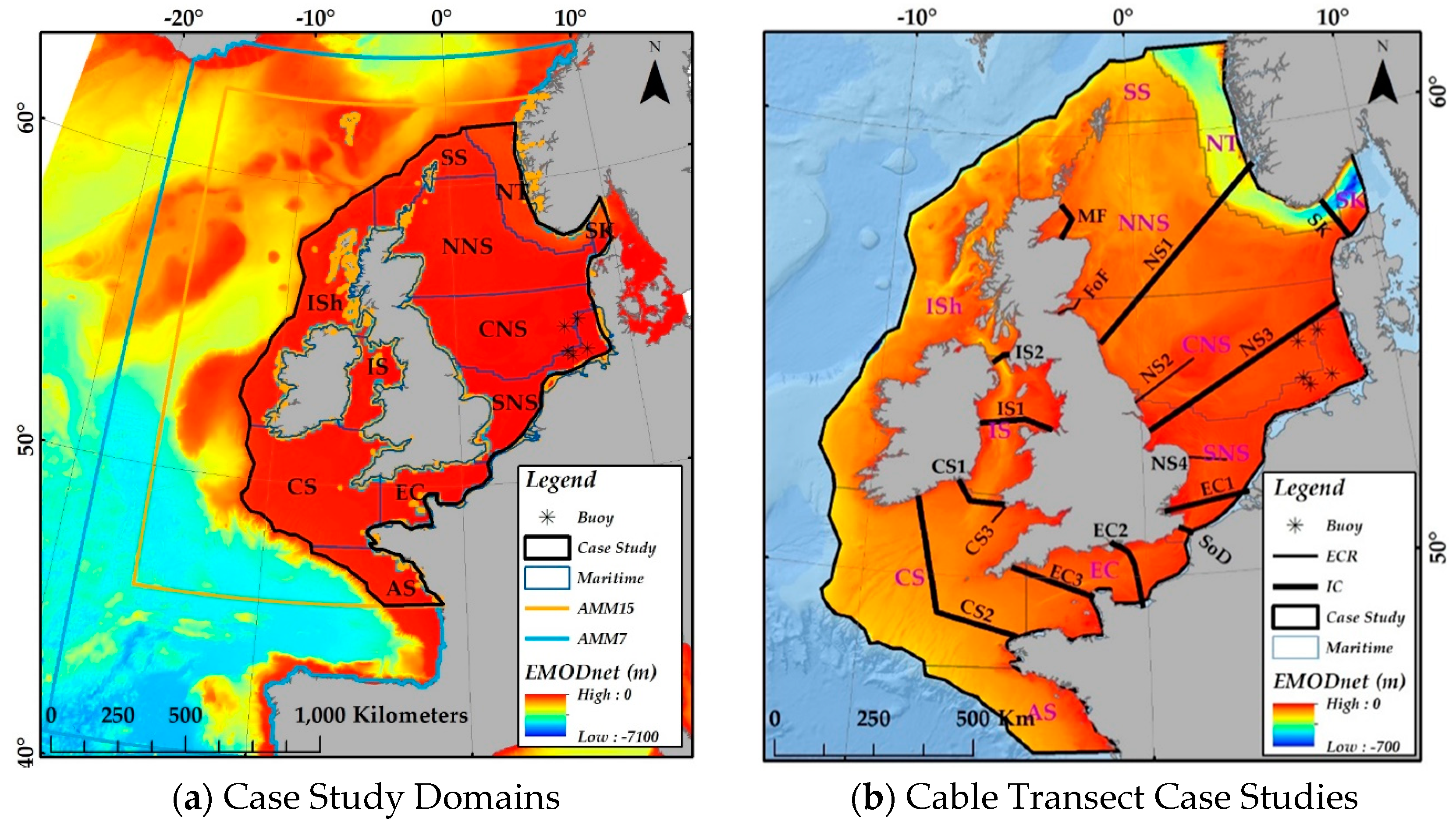
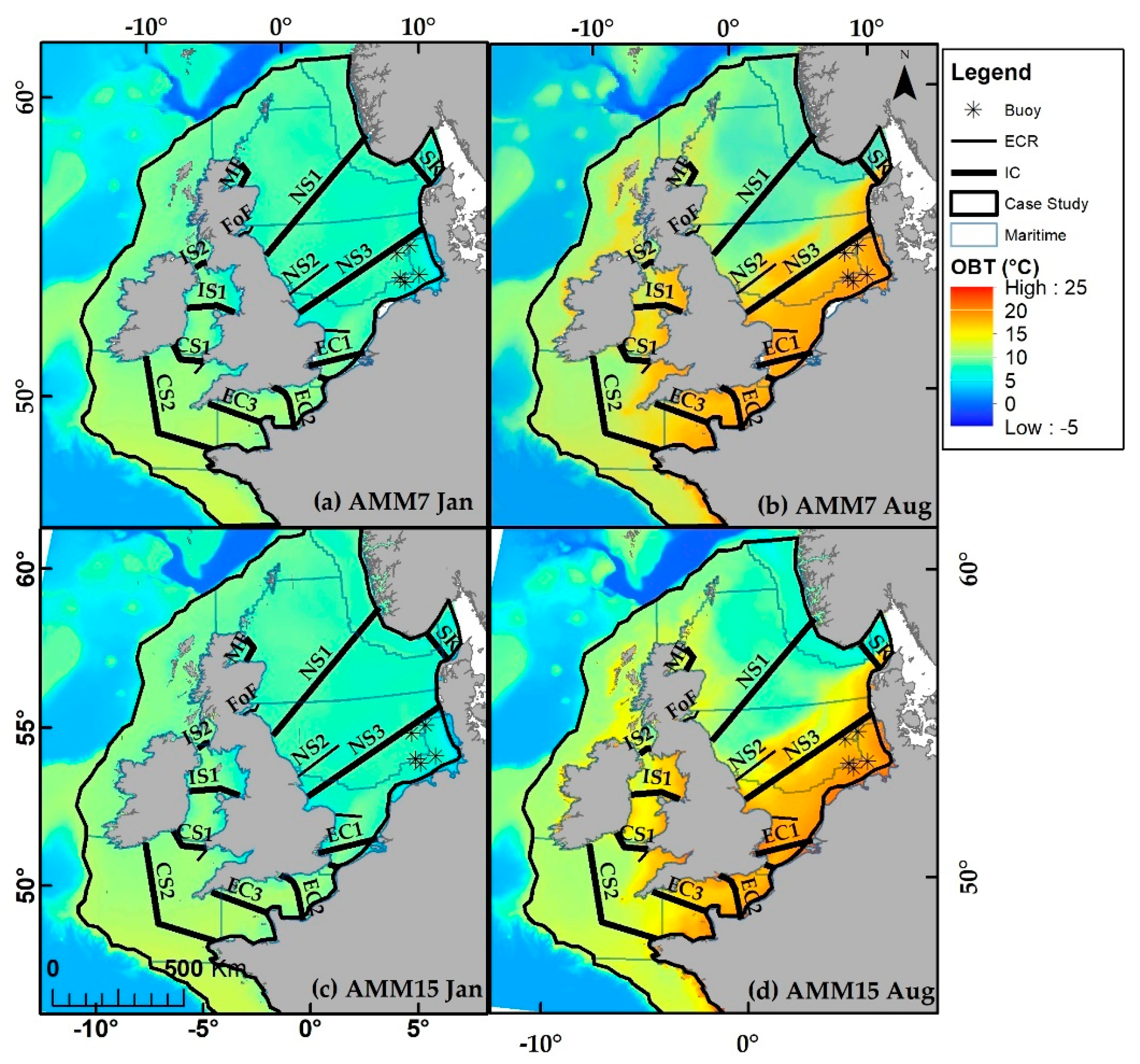
4. Spatial and Temporal Ambient Temperature Variation along Cable Routes

Having demonstrated the accuracy and the precision of the AMM7 and AMM15 models, the degree of spatial and temporal variability of OBT along individual cables routes can then be explored. For brevity, the AMM15 model, as it has a higher spatial resolution whilst retaining an accuracy comparable to the AMM7 one, has been preferentially used for the following analysis. A series of 16 theoretical cable routes have been defined (Figure 2 and Figure 3), and the monthly OBTs have been extracted for each of them (Figure 8). These data have then been used to calculate the maximum, minimum, mean, and standard deviation OBTs (along with percentile statistics) for both models for each route (Table 2).
Maximum annual OBTs vary from 13.3 °C (NS1) to 20.8 °C (EC2), with Figure 8 clearly demonstrating that the common use of 15 °C for cable design is far from capturing the true variation in ambient OBT. If considered purely in terms of the maximum temperature encountered during a year, this standard value underestimates all the maximum OBTs bar 1 (NS1) of the routes, which overestimates the temperature by 1.7 °C. Only three routes are within 1 °C of this standard value (IS2, CS2, and MF), with the rest exceeding it by between 1.4 and 5.8 °C. Similarly, the annual range of OBTs that each cable encounters over a year varies significantly, too, and is between 7.0 °C (NS1) and 15.9 °C (NS3).
These differences are not purely driven by the geographical location of the cables, as even neighboring cables (e.g., cables NS1 and NS2, which are only ~170 km apart, as seen in Figure 3) can experience very different temperature ranges. For instance, NS2 has a maximum temperature of 2.7 °C greater than NS1, with a range differential of +4.8 °C.
To further demonstrate the implications of spatially and temporally varying ambient temperature, mean monthly AMM15 OBTs were plotted for three cables: EC2, NS1, and SK (Figure 9). The EC2 and NS1 cables represent the most and least thermally onerous of the 16 transects, whilst the SK one has the largest (>400 m) bathymetry variation along the cable. Minimum mean monthly OBTs occurring between February and April are relatively stable along each transect, with values of 8.4 ± 0.88 °C (EC2 @ 1 STDEV), 6.95 ± 0.21 °C (NS1 @ 1 STDEV), and 5.97 ± 0.78 °C (SK @ 1 STDEV). Conversely, the maximum mean monthly AMM15 OBTs occur between August and October and can vary significantly along and between routes with EC2, having higher temperatures but limited variability 18.53 ± 0.73 °C (@ 1 STDEV), whilst NC1 and SK exhibit lower maximums but increasing variability with values of 9.55 ± 1.15 °C (@ 1 STDEV) and 11.52 ± 4.44 °C (@ 1 STDEV), respectively. The well-mixed shallow (<50 m) waters of EC2 demonstrate strong seasonal variation, whilst the wide-ranging water depths of SK (20–550 m) result in the shallow sections of the route having similar seasonal variation as EC2, and the deep waters of the Norwegian Trench, meanwhile, promote seasonal thermal stratification and thus retain cold low variability signatures throughout the year (Figure 9). The more northerly location of the NS1 cable and the deeper overall water depths, except for the coastal margin, result in relatively low temperatures and low variability throughout the year and along the whole route (Figure 9).
Such temperature variation, both between different cables and along individual cable routes, shows that a single value simply cannot be used for the design of an individual cable. As cable lengths of both export cables and interconnectors increase, the use of multi-cable segment designs becomes more prevalent. Consequently, utilizing the ambient temperature measurements from such whole shelf models could provide critical input to a segmented cable design. Furthermore, this demonstrates that a single site deployment of an ocean bottom temperature sensor would not resolve these cable design issues, since, in many cases, they would fail to capture the range of the temperature present on an individual route.

5. Implications for Cable Rating

The implications of ambient OBT estimates on cable design can be evaluated through modelling the operating conductor temperature using a 1D numerical cable model [16]. This model has the capability of considering conductive and convective heat transfer within sediments, solving governing equations for pressure and temperature within an annular domain with an inner diameter equivalent to the cable and an outer diameter equal to four times the burial depth. The equations are solved numerically using a second order central finite difference scheme spatially with backwards Euler time stepping. Within the cable, temperature is calculated using a standard RC thermal network model, with continuity of temperature and heat flux at the cable boundary. It should be noted that for the purposes of the investigations conducted here, convective heat transfer is negligible and the model performance is equivalent to that using standard RC thermal network models for the entire computational domain (cable and sediment), which are well established in the literature (e.g., [37]). Dynamically varying ambient temperature at cable depth is explicitly included in conductor loss calculations that depend on absolute temperature, but it is otherwise added to the conductor temperature rise above ambient at the end of the calculation.
Given the length of the case study routes (Figure 2 and Figure 3), a 500 kV HVDC bipole configuration was utilized to be more indicative of similar extant installations. Within the model, the bipole configuration was treated as a single equivalent conductor. This implementation was validated using an FEA model, which considered the full bipole arrangement. The burial depth of the cable was set to 1 m. The sediment thermal conductivity was 1.43 W/mK, equivalent to a thermal resistivity of 0.7 Km/W, which is the “standard” frequently used in cable design for marine sediments [7]. The volumetric heat capacity of the sediment was set to 2 × 10⁶ (J·K−1·m−3), which is a typical value for marine sediments [38].
To demonstrate the impact of ambient temperature assumptions on conductor temperature and cable ratings, a suite of static and dynamic ratings are calculated for two locations along each of the three case study cable routes (EC2, NS1 and SK). The locations are chosen to represent thermal extremities, i.e., sites indicative of higher (annotated A in Figure 9) and lower (annotated B) OBTs along the route. The dynamic rating was determined using a two-year normalized synthetic power curve time series, scaling it by a suitable maximum current (1844 A) until a maximum conductor temperature of 70 °C was reached, which is the typical maximum operating temperature for HVDC cables. The power curve is derived from typical wind power generation data, and, as such, the maximum conductor temperature is often not reached in the winter months, which corresponds to lower ambient temperatures at cable depth due to the higher generation (an example of this is provided in Figure 10).
The impact of using different ambient temperature inputs on cable design is demonstrated through both the generation of conductor temperature plots (Figure 11 and Figure 12) and cable rating statistics (Table 3). These results are provided for a range of ambient temperature scenarios, including:
  • A fixed ambient temperature of 15 °C, which is commonly used in commercial projects and used as a base level for comparison.
  • A fixed ambient temperature of the maximum OBT.
  • A fixed ambient temperature of the mean OBT.
  • An OBT time series, which is the most indicative of the true conditions at each site.
Figure 11 shows the conductor temperature time-series for a full year for all of the six modelled locations. For localities EC2-A, EC2-B, NS1-A, and SK-A, there are clearly significant differences in conductor temperature between the four different OBT input runs, whilst for NS1-B and SK-B, there is only a visible difference between the S15 run and the others. This is in response to the location of NS1-B and SK-B in deeper continental shelf waters (depths of −230 m and −500 m, respectively), which have overall lower OBTs (<7.9 °C) with almost no seasonal variation (Figure 11d,f). These plots also show the OBT time-series (blue dashed line) and the ambient temperature at actual cable depth (blue solid line—POBT). The comparison of these two in Figure 11a–c,e clearly demonstrates that the temperature variation at depth is both ameliorated and offset, with a lag of ~2–3 weeks. This offset, when combined with the load profile, results in additional temporal variations in conductor temperature compared to the static calculations.
This temperature propagation effect can be more clearly seen in Figure 12. These plots represent the difference between each model runs conductor temperature and the conductor temperature time-series calculated for S15. For SMax and SMean, the differential is effectively a static shift of within a range of ± 10 °C. However, the dynamic model runs for EC2-A, EC2-B, SK-A, and NS1-A (Figure 11a–c,e) exhibit time-varying differentials that are clearly in phase with the ambient temperature at cable depth but out of phase with the input OBT. For NS1-A and SK-A, the temperature differential fluctuates over the year: it is cooler during the winters and slightly warmer during the summers. It is important to note that due to the seasonal variation in load, this does not result in the maximum conductor temperature of 70 °C being exceeded, since the highest temperature differentials occur in September when the loads and overall conductor temperatures are lower.
CC1D has also been used to quantify the percentage difference in cable rating between the static S15 calculation and the other model runs (Table 3) for the six test locations, with a total of 24 comparisons. Three runs (EC2-A Max OBT, EC2-B Max OBT, and SK4-A Max OBT) show that using a fixed 15 °C ambient temperature overrates the cable by between 2.5 and 4.1%, which suggests that the potential for overheating could be increased and that the cable may be at risk. By contrast, when a static maximum OBT is used for NS1-A, NS1-B, and SK-B, this underrates the cable by between 2.6 and 7.5%, which suggests that these cables could handle an increased load or, if considering segmented cable sections, that a reduction in the cross-sectional area for the cable design at this location could be implemented.
When a static mean OBT is used, all of the relevant model runs suggest that there would be a rating increase of between 1.7 (EC2-B) and 7.6% (SK4-B). However, we would question how representative the Mean of the Monthly Mean OBT values are for cable design as they will potentially not capture, shorter lived but potentially significantly extreme values. Ultimately, sensitivity modelling should be undertaken in order to establish whether the ratings gain is suitably offset by the potential risk of exceeding long-term temperature.
As demonstrated by studies on the impact of time-varying OBT on real-time export cable rating optimization [19], using time varying OBT time series will provide the most realistic ambient temperature conditions that the cable will encounter. The ratings based on the OBT time series all show an increase relative to the S15 static runs. For the EC2 cable, these represent relatively small gains of 0.8 and 1.4% for the low and high thermal scenarios due to the overall higher ambient temperature that is encountered along the entire length of this cable. By contrast, for the NS1 and SK4 cables, gains of between 3% (SK4-A) and 7.8% (SK4-B) are registered. Again, such increases are significant in terms of either additional power transfer or considering a change in cable cross-sectional for all or part of the cable route.

6. Discussion

This paper demonstrates that properly capturing ambient ocean bottom temperature from publicly available resources can result in either a significant increase in cable rating or the identification of potentially high-risk overrated sections compared with ratings based on commonly used fixed temperature values (e.g., 15 °C). A method for validating these OBT models against equally open access in situ observations has been presented and demonstrated on the AMM7 and AMM15 models of OBT across the Northwest European Shelf.
Analysis of these models demonstrates the scale of spatial and temporal variation that may be encountered by individual cable routes that transect this landscape. It has been demonstrated that individual cable routes can experience along-cable temperature variations of >12 °C at single points in time, whilst at single locations, they can experience temperature variations of >15 °C over the course of a year.
Using a 1D numerical cable model [16] with a fixed DC cable buried at a metre depth and in identical thermal ground conditions, the implications of OBT alone on cable rating have also been demonstrated. For the examples used, rating changes of between −4.1% and +7.8% were generated relative to a static 15 °C ambient model. It should be clear that this is a demonstrative exercise to show the impact of ambient temperature in isolation on submarine cable ratings, and in practice, it is obviously essential to consider both the spatial variation of sediment thermal properties (thermal resistivity and thermal diffusivity) as well as post-installation changes in depth of cover. However, as recent analysis of DTS data from active cables has shown [21], seasonal fluctuations have a primary control on actual cable temperatures.
As cable routes become longer, either through greater transit lengths of interconnectors (e.g., XLinks, 3800 km) or expansion into deeper water and the further offshore fixed and floating windfarms, the design of segmented cables can be optimized by fully considering the whole thermal environment.

7. Conclusions

  • A method is presented for validating publicly available ocean bottom temperature models with equally accessible in situ observations from global databases.
  • This validation method has been demonstrated on both the AMM7 and the AMM15 Northwest European Shelf physical models using 181,860, quality controlled, in situ measurements from the World Ocean Database.
  • The validation demonstrates that both models perform are similar to the whole shelf and whole year statistics of 1.25 ± 1.06 °C (@ 1 STDEV) MAE for the AMM7 model and 1.27 ± 1.08 °C (@ 1 STDEV) MAE for the AMM15 one. Model performance is temporally and spatially variable, with the models performing better in the winter (October–May: 1.09 °C ≥ MBE ≥ 0.61 °C; and 1.66 °C ≥ RMSE ≥ 1.38 °C) and worse in the summer (June–September: 1.48 °C ≥ MBE ≥ 1.17; 2.2 °C ≥ RMSE ≥ 1.69 °C). Spatially, the model has a positive bias in the East Central North Sea and the German Bight, and it has a negative bias at the outer shelf margins and in the Norwegian Trench.
  • Analysis of indicative cable routes across the Northwest European Shelf demonstrates that individual cable routes can experience along-cable temperature variations of >12 °C at single points in time, whilst at single locations, they can experience temperature variations of >15 °C over the course of a year.
  • 1-D numerical modelling based on a HVDC bipole at a fixed depth and with fixed thermal soil parameters demonstrates that considering the spatial and temporal variation in OBT can result in a cable rating change of −4.1% and +7.8% across six example case studies.
  • The magnitude of these variations demonstrate that a considered approach to OBT within cable models can result in both significant ratings (and hence capital expenditure and operating costs) gains and/or the avoidance of cable overheating. Further consideration of OBT does not require expensive additional in situ survey, but it can be confidently assessed from publicly available datasets with quantified uncertainties.

Author Contributions

Conceptualization, J.D. (Justin Dix); methodology, J.D. (Jon Duell), J.D. (Justin Dix) and H.P.; software, J.D. (Jon Duell) and G.C.; validation, J.D. (Jon Duell) and J.D. (Justin Dix); formal analysis, J.D. (Jon Duell), J.D. (Justin Dix) and G.C.; investigation, J.D. (Jon Duell) and J.D. (Justin Dix); resources, J.D. (Jon Duell); data curation, J.D. (Jon Duell); writing—original draft preparation, J.D. (Jon Duell), J.D. (Justin Dix) and G.C.; writing—review and editing, J.D. (Jon Duell), J.D. (Justin Dix), G.C. and T.H.; visualization, J.D. (Jon Duell); supervision, J.D. (Justin Dix), G.C. and T.H.; project administration, J.D. (Justin Dix); funding acquisition, J.D. (Justin Dix). All authors have read and agreed to the published version of the manuscript.

Funding

This research was funded by Natural Environmental Research Council (NERC); DTP2, Reference Number: NE/S007210/1.

Data Availability Statement

The data presented in this study are available on request from the corresponding author.

Acknowledgments

Understanding of and application of the ocean bottom temperature models was greatly improved through prompt and detailed conversations with COPERNICUS marine service (the model providers).

Conflicts of Interest

The authors declare no conflict of interest.

References

  1. Dix, J.K.; Hughes, T.J.; Emeana, C.J.; Pilgrim, J.A.; Henstock, T.J.; Gernon, T.M.; Thompson, C.E.L. Substrate Controls on the Life-Time Performance of Marine HV Cables. In Offshore Site Investigation Geotechnics 8th International Conference Proceeding; Society for Underwater Technology: London, UK, 2017; Volume 3, pp. 1–8. [Google Scholar]
  2. Zhao, X.; Liu, Y.; Wu, J.; Xiao, J.; Hou, J.; Gao, J.; Zhong, L. Technical and Economic Demands of HVDC Submarine Cable Technology for Global Energy Interconnection. Glob. Energy Interconnect. 2020, 3, 120–127. [Google Scholar] [CrossRef]
  3. Department for Business, Energy & Industrial Strategy. DUKES Digest of UK Energy Statistics Annual Data for UK, 2021; About This Release Information on Energy Production, Trade, and Consumption in the UK for Total Energy and by Specific Fuels; Department for Business, Energy & Industrial Strategy: London, UK, 2021; pp. 2–5. [Google Scholar]
  4. The Crown Estate. The Crown Estate Offshore Wind Report 2021; The Crown Estate: London, UK, 2021; pp. 1–49. [Google Scholar]
  5. BESS. British Energy Security Strategy. Gov.UK. 2022; pp. 1–33. Available online: https://assets.publishing.service.gov.uk/government/uploads/system/uploads/attachment_data/file/1069969/british-energy-security-strategy-web-accessible.pdf (accessed on 16 July 2023).
  6. Thomas, B.; McKee, N.J.D.; Kleist, J. Analysis of Standardized Precipitation Index (SPI) Data for Drought Assessment. Water 1993, 26, 1–72. [Google Scholar]
  7. IEC60287-1-1; Electric Cables—Part 1-1: Current Rating Equations (100% Load Factor) and Calculation of Losses—General. International Electrotechnical Commission: Geneva, Switzerland, 2023.
  8. Worzyk, T. Submarine Power Cables: Design, Installation, Repair, Environmental Aspects; Springer: Berlin/Heidelberg, Germany, 2009. [Google Scholar] [CrossRef]
  9. Brakelmann, H.; Anders, G.J. Current Rating Considerations in Designing HVDC Cable Installations. IEEE Trans. Power Deliv. 2018, 33, 2315–2323. [Google Scholar] [CrossRef]
  10. de León, F.; Anders, G.J. Effects of Backfilling on Cable Ampacity Analyzed with the Finite Element Method. IEEE Trans. Power Deliv. 2008, 23, 537–543. [Google Scholar] [CrossRef]
  11. Anders, G.J. Rating of Electric Power Cables in Unfavorable Thermal Environment; Wiley: Hoboken, NJ, USA, 2010; ISBN 9780471718741. [Google Scholar]
  12. Hanna, M.A.; Chikhani, A.Y.; Salama, M.M.A. Thermal Analysis of Power Cables in Multi-Layered Soil. IEEE Trans. Power Deliv. 1994, 9, 572–578. [Google Scholar] [CrossRef]
  13. Garrido, C.; Otero, A.F.; Cidrás, J. Theoretical Model to Calculate Steady-State and Transient Ampacity and Temperature in Buried Cables. IEEE Trans. Power Deliv. 2003, 18, 667–678. [Google Scholar] [CrossRef]
  14. Brakelmann, H.; Stammen, J. Thermal Analysis of Submarine Cable Routes: LSM or FEM? In Proceedings of the National Proceedings Power and Energy Conference (PECon), Putra Jaya, Malaysia, 28–29 November 2006; pp. 560–565. [Google Scholar] [CrossRef]
  15. De Lieto Vollaro, R.; Fontana, L.; Vallati, A. Thermal Analysis of Underground Electrical Power Cables Buried in Non-Homogeneous Soils. Appl. Therm. Eng. 2011, 31, 772–778. [Google Scholar] [CrossRef]
  16. Callender, G.; Ellis, D.; Goddard, K.F.; Dix, J.K.; Pilgrim, J.A.; Erdmann, M. Low Computational Cost Model for Convective Heat Transfer from Submarine Cables. IEEE Trans. Power Deliv. 2021, 36, 760–768. [Google Scholar] [CrossRef]
  17. Duraisamy, N.; Gooi, H.B.; Ukil, A. Ampacity Estimation for Submarine Power Cables Installed in Saturated Seabed-Experimental Studies. IEEE Trans. Ind. Appl. 2020, 56, 6229–6237. [Google Scholar] [CrossRef]
  18. Hughes, T.J.; Henstock, T.J.; Pilgrim, J.A.; Dix, J.K.; Gernon, T.M.; Thompson, C.E.L. Effect of Sediment Properties on the Thermal Performance of Submarine HV Cables. IEEE Trans. Power Deliv. 2015, 30, 2443–2450. [Google Scholar] [CrossRef]
  19. Hernandez Colin, M.A.; Dix, J.; Pilgrim, J. Export cable rating optimisation by wind power ramp and thermal risk estimation. IET Renew. Power Gener. 2021, 15, 1564–1581. [Google Scholar] [CrossRef]
  20. Werle, V.; Rouven, P.; Rathke, C.; Freitag, C.; Kumbartzky, G. Long term temperature measurements compared with transient calculation according to IEC 60853-2. In Proceedings of the JiCable 2019—10th International Conference on Insulated Power Cables, Paris, France, 23–27 June 2019; p. D7-4. [Google Scholar]
  21. Dix, J.; Rochat, E.; Rizzo, E. How understanding spatial and temporal variation of ocean bottom temperature can significantly enhance the interpretation of DTS data from marine HV cables. In Proceedings of the JiCable 2023, Lyon, France, 18–22 June 2023; p. A7-2. [Google Scholar]
  22. Müller, C.; Usbeck, R.; Miesner, F. Temperatures in Shallow Marine Sediments: Influence of Thermal Properties, Seasonal Forcing, and Man-Made Heat Sources. Appl. Therm. Eng. 2016, 108, 20–29. [Google Scholar] [CrossRef]
  23. King, R.R.; While, J.; Martin, M.J.; Lea, D.J.; Lemieux-Dudon, B.; Waters, J.; O’Dea, E. Improving the Initialisation of the Met Office Operational Shelf-Seas Model. Ocean Model. 2018, 130, 1–14. [Google Scholar] [CrossRef]
  24. Díaz, H.; Guedes Soares, C. Review of the Current Status, Technology and Future Trends of Offshore Wind Farms. Ocean Eng. 2020, 209, 107381. [Google Scholar] [CrossRef]
  25. Ardelean, M.; Minnebo, P. HVDC Submarine Power Cables in the World; Publications Office of the European Union: Luxembourg, 2015; ISBN 9789279527852. [Google Scholar]
  26. IEC60287-3-1; Electric Cables—Calculation of the Current Rating, Part 3-1: Operating Conditions—Site Reference Conditions. International Electrotechnical Commission: Geneva, Switzerland, 2017.
  27. Nielsen, T.V.M.; Jakobsen, S.; Savaghebi, M. Dynamic Rating of Three-Core XLPE Submarine Cables Considering the Impact of Renewable Power Generation. In Proceedings of the 2019 IEEE 13th International Conference on Compatibility, Power Electronics and Power Engineering (CPE-POWERENG), Sonderborg, Denmark, 23–25 April 2019. [Google Scholar] [CrossRef] [Green Version]
  28. Tonani, M.; Pequignet, C.; King, R.; Sykes, P.; Mcconnell, N.; Siddorn, J. North West European Shelf Production Centre NORTHWESTSHELF_ANALYSIS_FORECAST_PHYS_004_013; Copernicus Marine Service: Toulouse, France, 2021; pp. 1–46. [Google Scholar]
  29. Tonani, M.; Sykes, P.; King, R.R.; McConnell, N.; Péquignet, A.C.; O’Dea, E.; Graham, J.A.; Polton, J.; Siddorn, J. The Impact of a New High-Resolution Ocean Model on the Met Office North-West European Shelf Forecasting System. Ocean Sci. 2019, 15, 1133–1158. [Google Scholar] [CrossRef] [Green Version]
  30. Graham, J.A.; O’Dea, E.; Holt, J.; Polton, J.; Hewitt, H.T.; Furner, R.; Guihou, K.; Brereton, A.; Arnold, A.; Wakelin, S.; et al. AMM15: A New High-Resolution NEMO Configuration for Operational Simulation of the European North-West Shelf. Geosci. Model Dev. 2018, 11, 681–696. [Google Scholar] [CrossRef] [Green Version]
  31. Cowley, R.; Killick, R.E.; Boyer, T.; Gouretski, V.; Reseghetti, F.; Kizu, S.; Palmer, M.D.; Cheng, L.; Storto, A.; Le Menn, M.; et al. International Quality-Controlled Ocean Database (IQuOD) v0.1: The Temperature Uncertainty Specification. Front. Mar. Sci. 2021, 8, 689695. [Google Scholar] [CrossRef]
  32. Good, S.A.; Martin, M.J.; Rayner, N.A. EN4: Quality Controlled Ocean Temperature and Salinity Profiles and Monthly Objective Analyses with Uncertainty Estimates. J. Geophys. Res. Ocean. 2013, 118, 6704–6716. [Google Scholar] [CrossRef]
  33. Morris, D.J.; Pinnegar, J.K.; Maxwell, D.L.; Dye, S.R.; Fernand, L.J.; Flatman, S.; Williams, O.J.; Rogers, S.I. Over 10 Million Seawater Temperature Records for the United Kingdom Continental Shelf between 1880 and 2014 from 17 Cefas (United Kingdom Government) Marine Data Systems. Earth Syst. Sci. Data 2018, 10, 27–51. [Google Scholar] [CrossRef] [Green Version]
  34. Garcia, H.E.; Boyer, T.P.; Locarnini, R.A.; Baranova, O.K.; Zweng, M.M. World Ocean Database 2018: User’s Manual (Prerelease); Mishonov, A.V., Ed.; NOAA: Silver Spring, MD, USA, 2018; Volume 12, pp. 29–34. [Google Scholar]
  35. Cheng, L.; Abraham, J.; Goni, G.; Boyer, T.; Wijffels, S.; Cowley, R.; Gouretski, V.; Reseghetti, F.; Kizu, S.; Dong, S.; et al. XBT Science: Assessment of Instrumental Biases and Errors. Bull. Am. Meteorol. Soc. 2016, 97, 923–933. [Google Scholar] [CrossRef]
  36. Moumena, A.; Guessoum, A. Fast Anomaly Detection Using Boxplot Rule for Multivariate Data in Cooperative Wideband Cognitive Radio in the Presence of Jammer. Secur. Commun. Netw. 2015, 8, 212–219. [Google Scholar] [CrossRef]
  37. Diaz-Aguiló, M.; De León, F.; Jazebi, S.; Terracciano, M. Ladder-type soil model for dynamic thermal rating of underground power cables. IEEE Power Energy Technol. Syst. J. 2014, 1, 21–30. [Google Scholar] [CrossRef]
  38. Goto, S.; Yamano, M.; Morita, S.; Kanamatsu, T.; Hachikubo, A.; Kataoka, S.; Tanahashi, M.; Matsumoto, R. Physical and thermal properties of mud-dominant sediment from the Joetsu Basin in the eastern margin of the Japan Sea. Mar. Geophys. Res. 2017, 38, 393–407. [Google Scholar] [CrossRef] [Green Version]
Figure 1. Example of ampacity model input IEC-60287 considering cable properties as well as operational, geometric, and environmental factors.
Energies 16 05454 g001
Figure 2. (a) This paper’s case study domain is broadly defined by the 200 m bathymetric contour, the AMM7 and AMM15 ocean bottom temperature model domains, and EMODnet bathymetry for the Northwest European Shelf. The case study domain has been sub-divided into 11 maritime domains: the North North Sea (NNS), the Central North Sea (CNS), the South North Sea (SNS), the English Channel (EC), the Celtic Sea (CS), the Irish Sea (IS), the Irish Shelf (ISh), the Shetland Shelf (SS), the Norwegian Trench (NT), Skagerrak (SK), and the Armorican Shelf (AS). (b) This map shows the locations of the “indicative” marine interconnector and export cables routes used in this paper: the Moray Firth (MF), the Firth of Forth (FoF), the North Sea (NS1 to 4), Skagerrak (SK), the Straits of Dover (SoD), the English Channel (EC1 to 3), the Celtic Sea (CS1 to 3), and the Irish Sea (S1 and S2).
Energies 16 05454 g002
Figure 3. Annual mean monthly modelled ocean bottom temperature variability for January (a,c) and August (b,d) for the AMM7 (a,b) and AMM15 (c,d) models. The primary time-series datasets used to calibrate both models are also shown [29].
Energies 16 05454 g003
Figure 4. This demonstrates the (a) pre-QC and (b) post-QC differences for AMM7 (blue) and AMM15 (yellow) modelled ocean bottom temperature for the whole domain (ALL) as well as the monthly values. Data distributions are represented using violin boxplots, which demonstrate kernel density distribution. The mean is plotted as an (*). Orange and red dashed lines in both (a,b) represent the soft and extreme anomaly boundaries, respectively, for the Pre-QC dataset, with extreme anomalies removed in (b).
Energies 16 05454 g004
Figure 5. Monthly distribution of observations color coded by measurement device of the final (post-QC) 181,860 ocean bottom temperature observations derived from WOD observations within the case study domain. Moorings used to produce the initial calibration are highlighted [29,30]. OSD = Ocean Station Data; CTD = Conductivity, Temperature and Depth profiler; XBT = Expendable Bathythermograph; MBT = Mechanical Bathythermograph; MRB = Moored Buoy; APB = Autonomous Pinniped Bathythermograph; GLD = Gliders; and PFL = Profiling Float.
Energies 16 05454 g005
Figure 6. Stacked bar charts demonstrating temporal distribution, monthly (top) and decadal (bottom), of the different measurement devices used in the final (post-QC) 181,860 ocean bottom temperature observations within the case-study domain. Instrument definitions were as per Figure 5. Some instruments such as PFL occure comparitively infrequently and consequently they are are not easily distinguished on this figure.
Energies 16 05454 g006
Figure 7. The distribution of normalized mean monthly OBT Bias Errors for AMM7 (a) and AMM15 (b) using the post-QC WOD dataset.
Energies 16 05454 g007
Figure 8. Violin-boxplots demonstrating AMM15 annual mean monthly OBT distributions for 16 theoretical cable routes (Figure 2 and Figure 3). Distribution statistics are tabulated in Table 2. Boxplots demonstrate the P25th–P75th percentiles, and the mean (*) and median (-) violin plots demonstrate the OBT density distribution for the whole cable. The red 15 °C line represents a typical static conservative estimate of ambient OBT [26].
Energies 16 05454 g008
Figure 9. Indicative cable route transects of AMM15 OBT and EMODnet bathymetry for the EC2 (top), NS1 (middle), and SK (bottom) cables. The common static value (15 °C) is also plotted. OBT data from locations A and B (highlighted with an asterisk on each route) are used for the cable conductor temperature and rating calculations described in Section 5.
Energies 16 05454 g009
Figure 10. Synthetic dynamic load time series limited to a maximum load of 1844 A.
Energies 16 05454 g010
Figure 11. Conductor temperature modelled using CC1D, with the load time series shown in Figure 10, for higher (A) and lower (B) thermal scenarios for the case study transects EC2 (a,b), NS1 (c,d), and SK1 (e,f). Static (S) ambient OBT inputs include 15 °C (S15) as well as SMax and SMean, whilst DOBT is generated using an annual OBT time series. The input OBT time series is shown as the blue dashed line along with the propagated temperature at cable depth (POBT—blue solid line).
Energies 16 05454 g011
Figure 12. Conductor temperature differential between each model run (Smax, SMean, and DOBT) and the “commonly used” S15 output. Results for the higher and lower thermal scenarios for EC2 (a,b), NS1 (c,d), and SK (e,f) are provided. The input OBT time series is shown as the blue dashed line along with the propagated temperature at cable depth (POBT—blue solid line).
Energies 16 05454 g012
Table 1. AMM7 and AMM15 MBE, σMBE, MAE, σMAE and RMSE validation statistics for each month and the whole year (‘All’). Bold values indicate which out of the AMM7 and the AMM15 has the best validation metric both for all and monthly. Red indicates the worst errors.
Pre-QCAMM7AMM15
MonthnMBEσMBEMAEσMAERMSEMBEσMBEMAEσMAERMSE
All182,6371.081.351.291.151.721.051.331.281.121.70
January13,3180.971.161.121.031.521.041.21.171.071.59
February18,9010.71.160.980.941.360.651.190.970.951.36
March12,4211.11.281.261.121.680.921.291.161.071.58
April12,2770.961.211.131.041.540.771.191.020.981.42
May18,0250.821.31.210.941.530.851.251.190.941.51
June17,3401.311.331.481.131.861.181.281.371.081.74
July19,1441.481.661.651.52.231.371.581.561.42.09
August20,5891.411.411.541.261.991.41.371.531.221.96
September16,8811.271.381.421.231.881.411.41.531.271.99
October13,8440.821.211.130.921.460.941.231.220.951.55
November12,3900.991.241.181.061.591.041.241.221.061.61
December75070.681.191.020.921.370.661.21.020.921.37
Post-QCAMM7AMM15
All181,8601.031.271.251.061.641.061.291.271.081.67
January13,21311.091.130.951.480.941.051.080.911.41
February18,7850.611.120.940.871.280.671.090.950.861.28
March12,3970.911.261.151.051.561.091.251.251.091.66
April12,2020.751.110.990.911.340.931.131.10.971.47
May18,0070.851.241.180.931.50.821.291.210.931.52
June17,3181.171.261.361.051.721.31.311.471.111.85
July19,1081.361.561.551.372.071.481.641.641.472.2
August20,4801.381.291.51.141.881.381.321.511.181.91
September16,6671.341.231.461.081.821.191.21.341.031.69
October13,8280.931.211.210.941.530.821.191.130.911.45
November12,3591.021.171.20.991.560.981.181.160.991.53
December74960.661.181.010.891.350.671.161.010.891.35
Table 2. Tabulated values quantifying the distribution statistics representing the AMM15 OBT variability along the cable transects (as shown in Figure 4).
Mean Monthly OBT Distribution and Variability (°C)
Transectsminmaxrangemeanp25p50p75iqrstdev
SK3.718.514.88.66.47.29.32.83.2
MF6.115.79.69.77.49.212.04.62.3
FoF5.216.411.29.77.09.512.35.22.6
NS 16.313.37.08.27.38.08.81.51.1
NS 25.317.011.810.37.59.912.75.23.0
NS 33.419.315.910.87.410.314.47.03.7
NS 45.318.413.111. 98.011.215.87.84.0
SoD7.019.412.412.99.212.216.37.13.7
EC 15.320.615.312.68.811.616.67.94.3
EC 26.720.814.213.19.812.416.46.73.6
EC 39.218.08.812.710.312.314.64.32.3
CS 18.216.58.211.49.511.112.83.32.1
CS 28.715.77.111.310.611.211.91.31.1
CS 38.316.78.412.09.511.713.94.42.4
IS 14.919.114.211.58.711.314.15.43.0
IS 27.115.38.210.98.610.813.14.52.4
Table 3. Dynamic cable rating results for different ambient temperature time series for all three cable routes and from examples of lower and higher thermal zones along each route.
Case StudyLocationScenarioAmbient OBTRatingRating % Difference from 15 °C
EC 2A: Thermal High15 °C fixed15.01844-
Mean OBT12.918781.8
Max OBT19.41768−4.1
OBT Time SeriesDynamic18691.4
B: Thermal Low15 °C fixed15.01844-
Mean OBT13.118761.7
Max OBT17.71797−2.5
OBT Time SeriesDynamic18580.8
NS1A: Thermal High15 °C fixed15.01844-
Mean OBT9.419375.0
Max OBT12.118922.6
OBT Time SeriesDynamic19254.4
B: Thermal Low15 °C fixed15.01844-
Mean OBT7.519676.7
Max OBT7.919596.2
OBT Time SeriesDynamic19646.5
SK4A: Thermal High15 °C fixed15.01844-
Mean OBT10.719153.9
Max OBT17.71798−2.5
OBT Time SeriesDynamic19003.0
B: Thermal Low15 °C fixed15.01844-
Mean OBT6.319857.6
Max OBT6.419837.5
OBT Time SeriesDynamic19877.8
Disclaimer/Publisher’s Note: The statements, opinions and data contained in all publications are solely those of the individual author(s) and contributor(s) and not of MDPI and/or the editor(s). MDPI and/or the editor(s) disclaim responsibility for any injury to people or property resulting from any ideas, methods, instructions or products referred to in the content.

