Implementation of Phasor Measurement Unit Based on Phase-Locked Loop Techniques: A Comprehensive Review

Abstract

The dynamic monitoring, control, and protection of modern power systems in real time require time-stamped electrical measurements to accurately estimate the bus voltage phasors using the state estimation function under normal and abnormal conditions. These measurements can be acquired by time-synchronized devices, known as phasor measurement units (PMUs). PMUs can measure bus voltage and branch current phasors of a three-phase network, as well as the frequency and the rate of change of frequency (ROCOF), with high speed, accuracy and time stamping provided by global positioning system (GPS) at the coordinated universal time (UTC). Various phasor estimation algorithms have been proposed in the literature, while most of them are concentrated in the discrete Fourier transform (DFT) algorithm, where an integer number of samples multiple of the nominal frequency is required for the computations. In cases where the frequency of the power grid deviates from its nominal value, the raw application of the DFT approach can lead to large errors during phasor estimation. Another approach of the phasor estimation is based on the phase-locked loop (PLL) techniques, widely used in grid tie inverters. PLL techniques can track dynamically (continuous time) the estimated frequency to the time-variant frequency of the power grid. A brief introduction to the basic concepts of the synchrophasor definition is provided, while the main DFT methods for synchrophasor estimation according to recent literature are mentioned. PLL-based PMU techniques are reviewed for both steady-state and dynamic conditions according to IEEE standards. In conclusion, the performance of PLL-based PMU algorithms presented in this literature review is discussed.

1. Introduction

So far, the majority of phasor estimation techniques that have been presented in literature can be divided into two main categories: (1) DFT-based and (2) non-DFT-based methods [1,2,3]. The former is used in the IEEE standard [4,5,6,7] due to its easy implementation and high robustness to the presence of harmonics [8]. The DFT-based methods work satisfactorily when the frequency of the signal under consideration is equal to the nominal frequency; otherwise, significant errors are induced due to the spectral leakage [9]. The interpolated DFT (IpDFT) algorithm and its modifications are widely used to address the spectral leakage issue [10], while further improvements of the IpDFT have been made in [11,12]. On the other hand, the non-DFT-based methods include several approaches, such as the Taylor–Kalman filters [13], recursive algorithm [14], weighted least squares (WLS) of a Taylor approximation [15], adaptive cascaded filters [16], polynomial Taylor–Fourier filters [17], Taylor–Fourier transform (TFT) [18], space vector (SV) approach [19,20] and phase-locked loop (PLL) algorithms [21,22,23,24,25,26,27].

The aforementioned PLL techniques, apart from being used in various industrial fields, are widely used to couple the grid tie converters to the utility network, with their main function of synchronizing the output frequency and phase angle with their input [28]. Despite their different approaches, PLL algorithms stem from a basic structure consisting of three main blocks [29] as depicted in Figure 1. The block diagram of the single-phase PLL comprises phase detection (PD), loop filter (LF) and voltage-controlled oscillator (VCO) blocks. The differences between the PLL algorithms focus on the PD block, due to its non-linearity [30]. The PD block determines the phase error between the input and output signals. This error signal becomes the input of the LF block, which represents the low-pass filter (LPF), providing the stability and the response of the overall PLL system. A first-order LPF or a proportional and integral (PI) controller is usually used to implement the LF block. In other words, the LF block defines the dynamics and the bandwidth of the system. The output signal of the LF block feeds into the VCO block which, in turn, produces an output signal which has the same phase compared to the input signal [31]. Therefore, the signal generated by the VCO block is synchronized with the input signal.

The purpose of this paper is to present and discuss the progress of recent research and different approaches considering the development and implementation of PLL-based PMU algorithms for synchrophasor estimation. Based on the examined challenges faced by phasor estimation methods, future work on such PLL-based PMU algorithms is proposed. This paper consists of five sections: In Section 2, the definition of synchrophasor concepts according to the IEEE standard is described, whereas the basic concepts of the three-phase PLL and challenges for their implementation are introduced in Section 3, for the sake of completeness. In Section 4, various PLL-based PMU approaches, proposed for addressing these challenges, are presented and mathematically analyzed, according to recent research. Finally, in Section 5, the aspects of this research field, based on the findings of the reviewed work, are summarized, and the paper is concluded.

2. Synchrophasor Concepts

The synchronized phasor requires a new consideration in addition to the classical concept of a phasor. The following equations provide the definition of the synchrophasor as described in the IEEE Std C37.118.1-2011 [4]. The sinusoidal waveform, derived from the voltage or the current of the power network, is presented in Equation (1), while it is a common practice to represent them in phasor form, as depicted in Equation (2), where the correlation of the phasor with the original signal is shown in Equation (3).

$$x\left(t\right)=X_m\mathit{cos}\left(\omega t+\phi \right)$$

(1)

$$\overline{X}=\frac{X_m}{\sqrt{2}}{e}^{j\phi }=\frac{X_m}{\sqrt{2}}\left[\mathit{cos}\left(\phi \right)+jsin\left(\phi \right)\right]=X_r+j{X}_i$$

(2)

$$x\left(t\right)=\mathcal{R}\left\{\sqrt{2}\overline{X}{e}^{j\omega t}\right\}$$

(3)

The rms value of the signal is represented by its magnitude $X_m/\sqrt{2}$, and $X_r$ and $X_i$ represent the real and imaginary parts of a complex value in the cartesian form, respectively. The value of phase angle $\phi$ depends on the time scale, at the time instant of $t=0$. Provided that the definition of the above phasor is based on the angular frequency $\mathsf{\omega }$, the elaboration with other phasors must be realized with the same frequency and time instant. The synchrophasor representation of signal $x\left(t\right)$ results from the abovementioned Equations (1) and (2), where $\phi$ is the difference between the instantaneous phase angle of $x\left(t\right)$ and a reference cosine signal running at the nominal frequency of the grid aligned to Coordinated Universal Time (UTC) [4]. Figure 2 depicts the convention for the angle $\phi$ in two different cases in order to define the angle offset of the synchrophasor based on the maximum positive value and positive zero crossing of the reference cosine signal occurring at the changeover of the UTC second (1 PPS time signal) [4].

Due to the nature of the power network, the frequency and amplitude of electrical signals are time-varying components; therefore, it is necessary to introduce new concepts to represent a synchrophasor. In the general case where the frequency and amplitude are time-dependent, the signal in Equation (1) can be rewritten as depicted in Equation (4):

$$x\left(t\right)=X_m\left(t\right)\mathit{cos}\left(2\pi f_{0}t+2\pi \int g\left(t\right)dt+\phi \right)$$

(4)

$$g\left(t\right)=f\left(t\right)-f_0$$

(5)

where $f_0$ and $f\left(t\right)$ are the nominal and the actual frequency, respectively, and $g\left(t\right)$ is the function of time that indicates the deviation of the actual from the nominal frequency. Therefore, the signal in Equation (4) can be represented as a synchrophasor depicted in Equation (6):

$$\overline{X}\left(t\right)=\frac{X_m\left(t\right)}{\sqrt{2}}{e}^{j\left(2\pi \int g\left(t\right)dt+\phi \right)}$$

(6)

Based on Equations (4)–(6), the actual frequency $f\left(t\right)$ and the rate of change of frequency $\mathrm{ROCOF}\left(\mathrm{t}\right)$ can be written as in the following Equations (7) and (8), respectively:

$$f\left(t\right)=f_0+\frac{1}{2\pi }\frac{d\phi }{dt}$$

(7)

$$ROCOF\left(t\right)=\frac{df\left(t\right)}{dt}=\frac{1}{2\pi }\frac{d^2\phi }{d{t}^2}$$

(8)

According to the IEEE standard [4,5,6,7], the accuracy of the synchrophasor estimation is defined by the total vector error (TVE) percentage which should not exceed 1% in steady-state conditions. The definition of the TVE is shown in Equation (9):

$$TVE\left(n\right)=\sqrt{\frac{{\left[{\hat{X}}_r\left(n\right)+X_r\left(n\right)\right]}^2+{\left[{\hat{X}}_i\left(n\right)+X_i\left(n\right)\right]}^2}{X_r{\left(n\right)}^2+X_i{\left(n\right)}^2}}$$

(9)

where the hats denote the sequences of the estimated values computed by the PMU under test, and the subscripts r and i indicate the real and imaginary parts of the phasor, respectively. Similarly, the values without hats denote the sequences of the theoretical values of the input signal at the instants of time (n).

The frequency and ROCOF errors between the measured and true values acquired at the same time should be evaluated using the following Equations (10) and (11).

$$FE=\left|f_{true}-f_{measured}\right|=\left|\Delta f_{true}-\Delta f_{measured}\right|$$

(10)

$$RFE=\left|{(\frac{df}{dt})}_{true}-{(\frac{df}{dt})}_{measured}\right|$$

(11)

where FE and RFE denote the frequency and ROCOF error measurement in Hz and Hz/s, respectively [4]. In order for a PMU to be compliant with the IEEE standard, various tests must be performed for the steady-state and dynamic conditions, as described in [4,5,6,7]. Depending on the scope and applicability of the PMUs, these tests are divided into two classes: P class and M class, for protection relays and measuring devices, respectively.

The required steady-state condition tests are performed by applying the following signals to the input of the PMU under test:

• Frequency step change test: A cosine signal with a frequency deviation of ±2 Hz for P class and ±5 Hz for M class of the nominal frequency.
• Magnitude deviation test: A cosine signal with an amplitude of 80% to 120% and 10% to 120% of the rated amplitude for P class and M class, respectively.
• Phase angle variation test: A cosine signal running at a frequency of $\left|f_{in}-f_{nominal}\right|<0.25 \mathrm{Hz}$ for both PMU classes.
• Harmonic distortion test: A signal containing 1% and 10% of each harmonic up to 50th for P class and M class, respectively.
• Out-of-band interference test: The frequency of the signal varies between nominal frequency and ±10% of half the frequency of the reporting rate. This test is applicable only for P-class PMU.

It should be noted that the maximum TVE for all steady-state tests is 1%, except for the out-of-band interference test where the maximum TVE value must not exceed 1.3%.

In terms of dynamic condition tests, the IEEE standard requires the input signal of the PMU under test to be modulated in amplitude, angle and frequency as follows:

• Amplitude modulation test: A cosine signal with a modulation amplitude of 10% of the rated amplitude value and modulation frequency of 2 Hz and 5 Hz for P class and M class, respectively.
• Phase angle modulation test: A cosine signal with a modulation angle of 0.1 radians and modulation frequency of 2 Hz and 5 Hz for P class and M class, respectively.
• Linear frequency ramp test: A cosine signal running at the nominal frequency by adding a frequency ramp of ±2 Hz/s and ±5 Hz/s for P class and M class, respectively.
• Magnitude step change test: A cosine signal with a 5% and 10% of the nominal magnitude step change for P class and M class, respectively.
• Phase angle step change test: A cosine signal with a 10° step change for both PMU classes.

The maximum TVE under a dynamic condition for the modulated amplitude and phase angle tests is 3%, and for the frequency ramp, the maximum TVE value must not exceed 1%. Furthermore, the PMUs shall report the synchrophasor measurements to the phasor data concentrators (PDCs) through communication channels at sub-multiples of the nominal power-line (system) frequency, also known as reporting rate measured in frames per second (FPS) [4].

3. Basic Concepts of the Three-Phase PLL

The single-phase PLL, presented in Figure 1, can be extended to a three-phase PLL to be used in a three-phase power system. Various PLL techniques have been proposed, and the basic structure used in three-phase systems is the synchronous reference frame (SRF)-PLL [31,32,33] depicted in Figure 3. In SRF-PLL, the three-phase balanced grid voltages $v_a\left(t\right)$, $v_b\left(t\right)$ and $v_c\left(t\right)$ of Equation (12) are first transformed into orthogonal signals $v_a\left(t\right)$ and $v_{\beta }\left(t\right)$ using the Clarke transformation in Equation (13), also called stationary reference frame. In continuation, the orthogonal signals are transformed into rotation reference frame $v_d\left(t\right)$ and $v_q\left(t\right)$ using the Park transformation [28] in Equation (14).

$$\left[v_{abc}\left(t\right)\right]=\left[\begin{array}{c}{v}_a\left(t\right)\\ v_b\left(t\right)\\ v_c\left(t\right)\end{array}\right]=V_m\left[\begin{array}{c}cos\left(\omega t\right)\\ cos\left(\omega t+\frac{2\pi }{3}\right)\\ cos\left(\omega t+\frac{4\pi }{3}\right)\end{array}\right]$$

(12)

$$\left[v_{\alpha \beta }\left(t\right)\right]=\left[\begin{array}{c}{v}_a\left(t\right)\\ v_{\beta }\left(t\right)\end{array}\right]=\left[T_{\alpha \beta }\right]\left[v_{abc}\left(t\right)\right]=\frac{2}{3}\left[\begin{array}{ccc}1& -\frac{1}{2}& -\frac{1}{2}\\ 0& \frac{\sqrt{3}}{2}& -\frac{\sqrt{3}}{2}\end{array}\right]\left[\begin{array}{c}{v}_a\left(t\right)\\ v_b\left(t\right)\\ v_c\left(t\right)\end{array}\right]$$

(13)

$$\begin{gathered} \left[v_{dq}\left(t\right)\right]=\left[\begin{array}{c}{v}_d\left(t\right)\\ v_q\left(t\right)\end{array}\right]=\left[T_{dq}\right]\left[v_{\alpha \beta }\left(t\right)\right]=\left[\begin{array}{cc}cos\left(\hat{\theta }\right)& sin\left(\hat{\theta }\right)\\ -sin\left(\hat{\theta }\right)& cos\left(\hat{\theta }\right)\end{array}\right]\left[\begin{array}{c}{v}_a\left(t\right)\\ v_{\beta }\left(t\right)\end{array}\right] \\ =V_m\left[\begin{array}{c}cos\left(\omega t-\hat{\theta }\right)\\ sin\left(\omega t-\hat{\theta }\right)\end{array}\right] \end{gathered}$$

(14)

where ${\mathrm{V}}_{\mathrm{m}}$ and $\mathsf{\omega }$ are the amplitude and the angular frequency of the grid voltages, respectively, and $\hat{\theta }$ is the estimated angle produced by the VCO section of the PLL scheme.

When the estimated angle $\hat{\theta }$ is close to the actual grid voltage angle $\mathsf{\omega }\mathrm{t}$ ($\omega t-\hat{\theta }$ is small enough), then the approximation $sin\left(\omega t-\hat{\theta }\right)\cong \omega t-\hat{\theta }$ is considered. Therefore, the $v_q$ component is linearly proportional to the difference $\left(\omega t-\hat{\theta }\right)$, and the PLL is locked when this difference is close to zero ($v_q\approx 0$), meaning that the PLL generates almost the same angle with the actual angle. In the next stage, the PI controller fed with the error signal $\left(\omega t-\hat{\theta }\right)$ produced by the closed-loop system attempts to set $v_q$ to zero maintaining the PLL locked. In the last section, an integrator is used for the computation of estimated angle $\hat{\theta }$.

Under nominal grid behavior, the SRF-PLL performs effectively, providing dynamically accurate phase angle and amplitude estimation. It is worth noting that in the three-phase balanced system, the dq components are practically dc components. In case the three-phase power network bears imbalances, the fundamental negative sequence acts on the $v_d$ and $v_q$ components as a signal with twice the actual frequency, rendering the estimated phase angle and amplitude inaccurate [34]. Advanced PLL algorithms have been proposed to mitigate the impact of the negative sequence derived from the grid imbalances focused on decoupling the fundamental positive-sequence components from the primary voltage signals [34].

4. PLL-Based Algorithm for the Estimation of the Synchrophasor

In this section, various proposed PLL-based PMU algorithms are presented, while the results of the steady-state and dynamic performance tests are summarized.

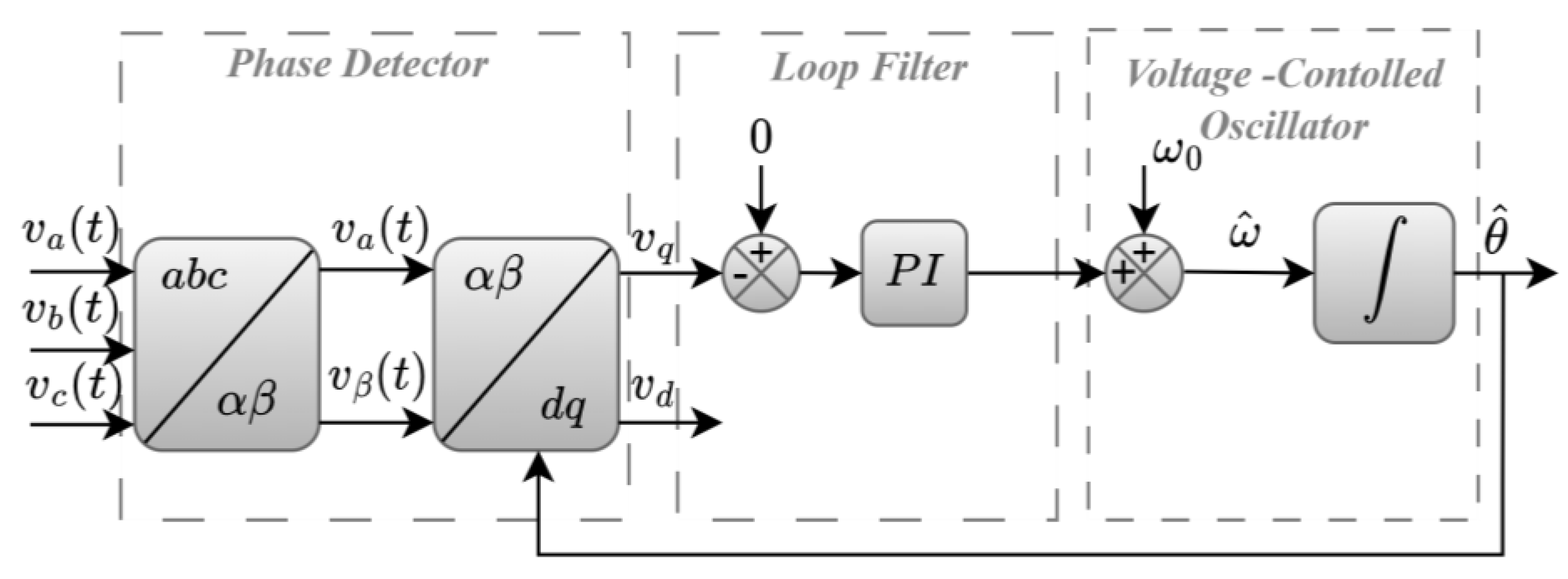
4.1. PID SRF-PLL-Based Algorithm for Positive-Sequence Synchrophasor Estimation

The authors in [35] implemented an SRF-PLL-based algorithm to estimate the positive sequence of the synchrophasor, employing the symmetrical components’ theorem of Fortescue introduced in [36]. A microcontroller unit (MCU) is used to examine the compatibility of the proposed algorithm with the IEEE standard [4,5,6,7] for classes P and M. In (15), the positive-, negative- and zero-sequence components are presented, where $x_a\left[n\right]$, $x_b\left[n\right]$, $x_c\left[n\right]$ are the instantaneous three-phase input signals sampled by the analog to digital converter (ADC) unit of the MCU with a sampling period $T$. The values $a^{+}\left[n\right]$, $a^{-}\left[n\right]$, $a^0\left[n\right]$, ${\phi }^{+}\left[n\right]$, ${\phi }^{-}\left[n\right]$, ${\phi }^0\left[n\right]$ are the instantaneous magnitudes and angles of the positive-, negative- and zero-sequence components, respectively, derived from the fundamental component of the three-phase input signal of the PLL.

$$\begin{gathered} \left[\begin{array}{c}{x}_a\left[n\right]\\ x_b\left[n\right]\\ x_c\left[n\right]\end{array}\right]=a^0\left[n\right]\left[\begin{array}{c}\mathit{cos}\left(\omega nT+{\phi }^0\left[n\right]\right)\\ cos\left(\omega nT+{\phi }^0\left[n\right]\right)\\ cos\left(\omega nT+{\phi }^0\left[n\right]\right)\end{array}\right]+a^{+}\left[n\right]\left[\begin{array}{c}\mathit{cos}\left(\omega nT+{\phi }^{+}\left[n\right]\right)\\ cos\left(\omega nT+{\phi }^{+}\left[n\right]-\frac{2\pi }{3}\right)\\ cos\left(\omega nT+{\phi }^{+}\left[n\right]+\frac{2\pi }{3}\right)\end{array}\right] \\ +a^{-}\left[n\right]\left[\begin{array}{c}\mathit{cos}\left(\omega nT+{\phi }^{-}\left[n\right]\right)\\ cos\left(\omega nT+{\phi }^{-}\left[n\right]+\frac{2\pi }{3}\right)\\ cos\left(\omega nT+{\phi }^{-}\left[n\right]-\frac{2\pi }{3}\right)\end{array}\right] \end{gathered}$$

(15)

At the beginning, the sampled three-phase input signals are transformed into a rotation reference frame (d-q) using the ABC-dq transform matrix depicted in Equation (16), which, in other words, is the Park transform matrix [20]. The d-q components obtained from the transformation ($x_{dq}\left[n\right]=T_{ABC\to dq}{x}_{abc}\left[n\right]$) are presented in Equation (17), where the zero-sequence component has been neglected.

$$T_{ABC\to dq}=\frac{2}{3}\left[\begin{array}{ccc}cos\left(\omega nT\right)& cos\left(\omega nT-\frac{2\pi }{3}\right)& cos\left(\omega nT+\frac{2\pi }{3}\right)\\ -sin\left(\omega nT\right)& -sin\left(\omega nT-\frac{2\pi }{3}\right)& -sin\left(\omega nT+\frac{2\pi }{3}\right)\end{array}\right]$$

(16)

$$x_{dq}\left[n\right]=a^{+}\left[n\right]\left[\begin{array}{c}\mathit{cos}\left({\phi }^{+}\left[n\right]\right)\\ \mathit{sin}\left({\phi }^{+}\left[n\right]\right)\end{array}\right]+a^{-}\left[n\right]\left[\begin{array}{c}\mathit{cos}\left(2\omega nT+{\phi }^{-}\left[n\right]\right)\\ \mathit{sin}\left(2\omega nT+{\phi }^{-}\left[n\right]\right)\end{array}\right]$$

(17)

It can be observed from Equation (17) that the negative-sequence component appears with twice the frequency on the rotating frame axis in case the three-phase input is unbalanced. Passing the d-q signals through a LPF finite impulse response (FIR) filter [23], the negative-sequence component is eliminated [37]. The filtered signal of q-component $y_q\left[n\right]$ after the normalization depicted in Equation (18) feeds the LPF block, where, in this case, is a proportional–integral–derivative (PID) controller that addresses the steady-state error and improves the dynamic response of the PLL. Applying the integral to the output of the PID controller, the estimated angle of the positive-sequence component is obtained and fed back to the ABC-dq matrix for the next computation. In case the PLL is locked, the q-component is close to zero; therefore, the estimated amplitude ${\hat{a}}^{+}\left[n\right]$ can be obtained from the filtered d-component $y_d\left[n\right]$.

$$e\left[n\right]=\frac{y_q\left[n\right]}{\sqrt{y_d^2\left[n\right]+y_q^2\left[n\right]}}$$

(18)

The estimated values of frequency and ROCOF are calculated at each reporting time interval $\Delta t$ of the proposed algorithm. The preliminary estimated frequency ${\hat{f}}_k^p$ of the utility is derived from (19), where ${\hat{\phi }}_k^{+}$ and ${\hat{\phi }}_{k-1}^{+}$ are the current and previous estimated positive-sequence angle, respectively, and $f_0$ is the nominal frequency. The ${\widehat{ROCOF}}_k$ is then calculated from (20) employing the current and previous values of the preliminary estimated frequency ${\hat{f}}_k^p$ and ${\hat{f}}_{k-1}^p$ obtained at each time interval $\Delta t$. Finally, the estimated frequency ${\hat{f}}_k^f$ is computed from Equation (21), where the correction factor ${\widehat{ROCOF}}_k/f_0$ is added to the preliminary estimated frequency. In Figure 4, the block diagram of the proposed SRF-PLL-based algorithm for positive-sequence synchrophasor estimation is presented where the hat denotes the corresponding estimated value.

$${\hat{f}}_k^p=f_0+\frac{1}{2\pi }\frac{{\hat{\phi }}_k^{+}-{\hat{\phi }}_{k-1}^{+}}{\Delta t}$$

(19)

$${\widehat{ROCOF}}_k=\frac{{\hat{f}}_k^p-{\hat{f}}_{k-1}^p}{\Delta t}$$

(20)

$${\hat{f}}_k^f={\hat{f}}_k^p+\frac{{\widehat{ROCOF}}_k}{f_0}$$

(21)

4.1.1. Experimental Results under Steady-State Conditions

The reporting rate used in this work is 25 FPS, and according to experimental results provided in [35], the proposed algorithm complies with the IEEE standard [4,5,6,7] for both classes P and M. Adding filters against input signal noise and harmonics presents positive results even in the out-of-band interference tests.

4.1.2. Experimental Results under Dynamic Conditions

The experimental results of the dynamic performance tests provided in [35] are as follows:

• Amplitude modulation test: The TVE is almost proportional to the value of the modulation frequency. Consequently, the TVE is considerably smaller for P class compared to M class since the required modulation frequency for P class is smaller than the corresponding M-class modulation frequency. Nevertheless, the proposed algorithm meets the requirement for both P and M classes.
• Phase angle modulation test: In this test, the proposed algorithm performs satisfactorily in terms of error values required by the standard making it compatible with both P and M classes.
• Linear frequency ramp test: The linear frequency ramp test results depict that the proposed algorithm fulfils all requirements for both PMU classes P and M.
• Amplitude step change test: The test results show that the TVE, FE and RFE narrowed very fast within the acceptable limits of the IEEE standard. Consequently, the proposed algorithm fulfils the requirements.
• Phase step change test: During the transient period, a small overshoot in the estimated signal amplitude occurred, causing phase and frequency errors that did not exceed the acceptable range for P and M classes.

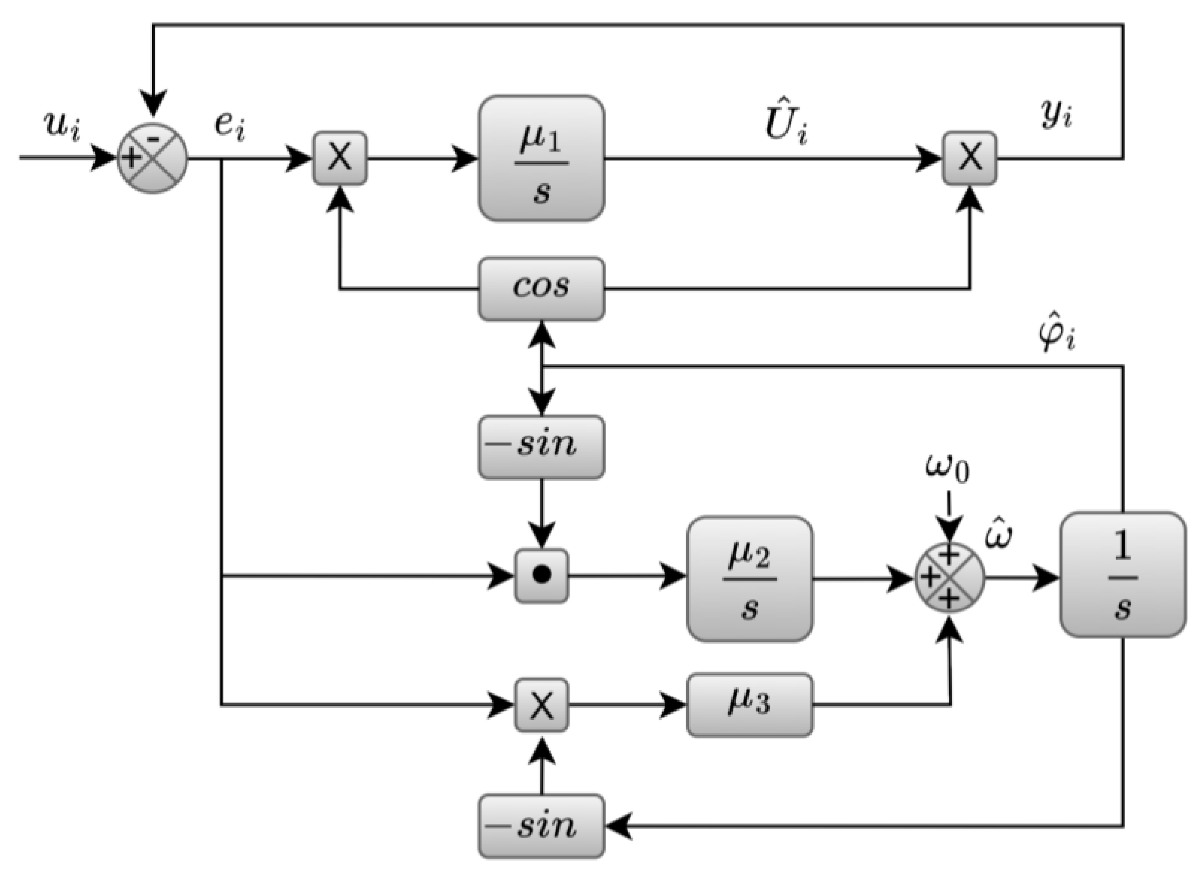
4.2. Three-Phase Enhanced PLL (EPLL)-Based Algorithm for Synchrophasor Estimation

The authors in [21] implemented a three-phase PLL-based algorithm for synchrophasor estimation, where the frequency and ROCOF are obtained by processing the estimated values of all three signals. The proposed three-phase PLL is derived from the extension of the single-phase EPLL in [2]. In Equation (22), the measured three-phase signals are depicted, while the corresponding filtered signals free from harmonics, inter-harmonics, switching ripples and noise are shown in Equation (23):

$$u\left(t\right)=\left[\begin{array}{c}{u}_a\left(t\right)\\ u_b\left(t\right)\\ u_c\left(t\right)\end{array}\right]=\left[\begin{array}{c}{U}_{a}cos\left({\phi }_a\right)\\ U_{b}cos\left({\phi }_b\right)\\ U_{c}cos\left({\phi }_c\right)\end{array}\right], {\phi }_i={{\displaystyle \int }}_0^t\omega \left(\tau \right)d\tau +{\delta }_i, i=a,b,c$$

(22)

$$\hat{u}\left(t\right)=\left[\begin{array}{c}{\hat{u}}_a\left(t\right)\\ {\hat{u}}_b\left(t\right)\\ {\hat{u}}_c\left(t\right)\end{array}\right]=\left[\begin{array}{c}{\hat{U}}_{a}cos\left({\hat{\phi }}_a\right)\\ {\hat{U}}_{b}cos\left({\hat{\phi }}_b\right)\\ {\hat{U}}_{c}cos\left({\hat{\phi }}_c\right)\end{array}\right], {\hat{\phi }}_i={{\displaystyle \int }}_0^t\hat{\omega }\left(\tau \right)d\tau +{\hat{\delta }}_i, i=a,b,c$$

(23)

where $U_i$ and ${\phi }_i$ for $i=a,b,c$ are the amplitudes and phase angle of the signals, and $\omega$ and ${\delta }_i$ for $i=a,b,c$ are the corresponding angular frequency of the system and the initial phase angle at time zero. The instantaneous error of the measured and the filtered signals is defined by the cost function depicted in Equation (24) [38].

$$J=\Vert u\left(t\right)-\hat{u}\left(t\right)\Vert {}^2={\left(u_a-{\hat{u}}_a\right)}^2+{\left(u_b-{\hat{u}}_b\right)}^2+{\left(u_c-{\hat{u}}_c\right)}^2$$

(24)

The differential equations shown in Equations (25)–(27) are obtained by applying the gradient descent method to the cost function. The parameters ${\mu }_1$, ${\mu }_2$ and ${\mu }_3$ are step sizes of the gradient descent method, and $e_i$ represents the error signal corresponding to $u_i-{\hat{u}}_a$ for $i=a,b,c$. The block structure of the proposed PLL is shown in Figure 5. The symbol × means that the multiplication of the input vectors is executed element-wise, while the dot symbol means that the multiplication of the input vectors is performed in vector format.

$${{\hat{U}}^{\prime }}_i={\mu }_1{e}_i\mathit{cos}{\hat{\phi }}_i, i=a,b,c$$

(25)

$${\hat{\omega }}^{\prime }=-{\mu }_2\left[e_{\alpha }\mathit{sin}\left({\hat{\phi }}_a\right)+e_b\mathit{sin}\left({\hat{\phi }}_b\right)+e_c\mathit{sin}\left({\hat{\phi }}_c\right)\right]$$

(26)

$${{\hat{\phi }}^{\prime }}_i=\hat{\omega }-{\mu }_3{e}_i\mathit{sin}\left({\hat{\phi }}_i\right), i=a,b,c$$

(27)

In Figure 5, the filtered signals are represented by $y_i$, and the vectors $U_i$ and ${\phi }_i$ denote the magnitudes and phase angles, respectively. It is observed from Equations (25)–(27) that factors ${\mu }_2$ and ${\mu }_3$ depend on the magnitudes $U_i$ for $i=a,b,c$, and for cases where the magnitudes fluctuate over a large range of values, the authors recommend the modification depicted in Equations (28)–(30) in order to maintain the system performance.

$${{\hat{U}}^{\prime }}_i={\mu }_1{e}_i\mathit{cos}{\hat{\phi }}_i, i=a,b,c$$

(28)

$${\hat{\omega }}^{\prime }=-{\mu }_2\left[\frac{e_{\alpha }\mathit{sin}\left({\hat{\phi }}_a\right)}{\left|{\hat{U}}_i\right|+\epsilon }+\frac{e_b\mathit{sin}\left({\hat{\phi }}_b\right)}{\left|{\hat{U}}_i\right|+\epsilon }+\frac{e_c\mathit{sin}\left({\hat{\phi }}_c\right)}{\left|{\hat{U}}_i\right|+\epsilon }\right]$$

(29)

$${{\hat{\phi }}^{\prime }}_i=\hat{\omega }-{\mu }_3\frac{e_i\mathit{sin}\left({\hat{\phi }}_i\right)}{\left|{\hat{U}}_i\right|+\epsilon }, i=a,b,c$$

(30)

where $\epsilon$ is a small positive number to avoid division by zero.

In Equations (31) and (32), the calculation of the positive-sequence phasor is depicted by considering the estimated magnitude $U_p$ and phase angle ${\phi }_p$ of the three-phase system obtained from the above proposed PLL. The use of the second-order linear bandpass filter (BPF) is recommended by the authors to attenuate undesirable noises obtained from the input signal shown in Equation (33). The proposed filter can block the dc component that may be introduced into the input signal, while high-frequency noises can be reduced with a trivial impact on the phase shift and magnitude distortion of the measured signal. Therefore, for the sake of accuracy, a compensation stage for the magnitude and phase angle is needed. Thus, the compensation is performed by employing the estimated angular frequency obtained from the proposed PLL as in Equation (34).

$$U_p=\left|\hat{M}\right|, {\phi }_p=\angle \hat{M}$$

(31)

$$\begin{gathered} \hat{M}=\frac{1}{3}\left[{\hat{U}}_{a}cos\left({\hat{\phi }}_a\right)+{\hat{U}}_{b}cos\left({\hat{\phi }}_b+\frac{2\pi }{3}\right)+{\hat{U}}_{c}cos\left({\hat{\phi }}_c\frac{2\pi }{3}\right)\right] \\ +j\frac{1}{3}\left[{\hat{U}}_{a}sin\left({\hat{\phi }}_a\right)+{\hat{U}}_{b}sin\left({\hat{\phi }}_b+\frac{2\pi }{3}\right)+{\hat{U}}_{c}sin\left({\hat{\phi }}_c\frac{2\pi }{3}\right)\right] \end{gathered}$$

(32)

$$H_{BPF}\left(s\right)=\frac{2\xi {\omega }_{0}s}{s^2+2\xi {\omega }_{0}s+{\omega }_0^2}$$

(33)

$$U_i^{comp}=\frac{U_i}{\left|H_{BPF}\left(j\hat{\omega }\right)\right|}, {\phi }_i^{comp}={\phi }_i-\angle H_{BPF}\left(j\hat{\omega }\right)$$

(34)

Moreover, a moving-average filter (MAF), to further attenuate undesired spikes from the magnitudes and frequency of the estimated signal, is recommended. In Figure 6, the block structure of the proposed phasor measurement algorithm is presented.

4.2.1. Simulation Results

In this section, the simulation results performed by the authors in [21] are summarized.

• Amplitude step change test: The initial three-phase balanced grid voltages undergo a step change of 10% of the fundamental amplitude. In steady-state conditions, the TVE value is below 1%. During the transient, the FE reaches 25 mHz, ROCOF reaches 4 Hz/s and the phase angle error reaches 1.25°.
• Phase angle step change test: The initial three-phase balanced grid voltages undergo a phase angle step change of 10°. In steady-state conditions, the TVE value is below 1%. During the transient, the FE reaches 100 MHz and ROCOF reaches 6 Hz/s. The phase angle is accurately detected.
• Frequency step change test: The initial three-phase balanced grid voltages undergo a frequency step change of 0.1 Hz. In steady-state and dynamic conditions, the TVE value is below 1%. During the transient, the ROCOF reaches 5 Hz/s and the phase angle error reaches 0.25°. The frequency step change is accurately detected.
• Linear frequency ramp test: The frequency of the grid voltages increases with a ramp function of 1 Hz/s. Under this dynamic behavior, the TVE is about 0.1%, the phase angle presents an error of 0.1°, and the frequency is tracked with a steady-state error of 20 MHz. It is worth mentioning that the ROCOF is accurately detected.
• Unbalanced Signal test: Negative- and zero-sequence components with a magnitude of 10% are induced in the three-phase balanced voltages. The PLL rejects the undesired components providing TVE less than 2% during transients and less than 1% in steady state.
• Harmonic distortion test: A signal containing 1% of each harmonic up to the 15th is induced in the three-phase balanced voltages. The TVE value is below 0.8%, the phase angle error is less than 0.5°, and no steady-state error has been observed in terms of frequency and ROCOF.
• Amplitude and Phase Modulation test: The modulation amplitude with a frequency of 2 Hz and a magnitude of 10% is applied to the PLL. The phase angle provides a peak error of about 0.25°, the FE is about 60 MHz, the peak value of RFE reaches 0.5 Hz/s and the TVE is almost 1%.

It should be mentioned that work [21] was first published in 2012, while the IEEE Standard for Synchrophasor Measurements for Power Systems, IEEE Std C37.118.1a-2014 (Amendment to IEEE Std C37.118.1-2011), was published later, resulting in some limits, which were used to be violated, as no longer being violated considering the latest revised standard.

4.2.2. Experimental Results

The authors in [39] implemented and tested the proposed algorithm on a 200 MHz digital signal processor (DSP) by making minor modifications to the original one. It is worth mentioning the low computational burden cost since the total execution time of the proposed algorithm is 21.6 μs. The two-area system proposed in [40] is used by the authors in order to test the proposed method in a more realistic scenario. The following test cases were simulated:

• Initially, the grid voltages are in normal condition when at time t = 0.5 s the following harmonics are injected into the grid: 5th, 7th, 11th and 13th, with the corresponding amplitude of 8%, 5%, 3% and 1% of the fundamental component. Under steady-state abnormal conditions, the TVE value is below 1%, FE is ±0.002 Hz and ROCOF is 40 Hz/s. The ROCOF value reaches 60 Hz/s during the transient period.
• Initially, the grid voltages are in normal condition when at the time t = 0.5 s a source voltage is connected to the network that bears an imbalance factor of 10% of the negative sequence. Under steady-state abnormal conditions, the TVE value is below 1%, FE is negligible and ROCOF is 0 Hz/s. The ROCOF value reaches 80 Hz/s during the transient period.
• In this test case, harmonics (from the first case) and low-frequency oscillations (of 1 Hz) are injected into the grid voltages. Under steady-state abnormal conditions, the TVE value is below 1%, while the ROCOF value reaches 40 Hz/s.
• In this final test case, all the above abnormal conditions are considered (harmonics, sequence unbalance and low-frequency oscillations). Under steady-state abnormal conditions, the TVE value is below 1%, while the ROCOF value reaches 30 Hz/s.

For all the above cases, it is observed that the proposed PLL provides low overshoots as well as a fast transient response for the respective measured values, such as amplitude, phase angle and frequency.

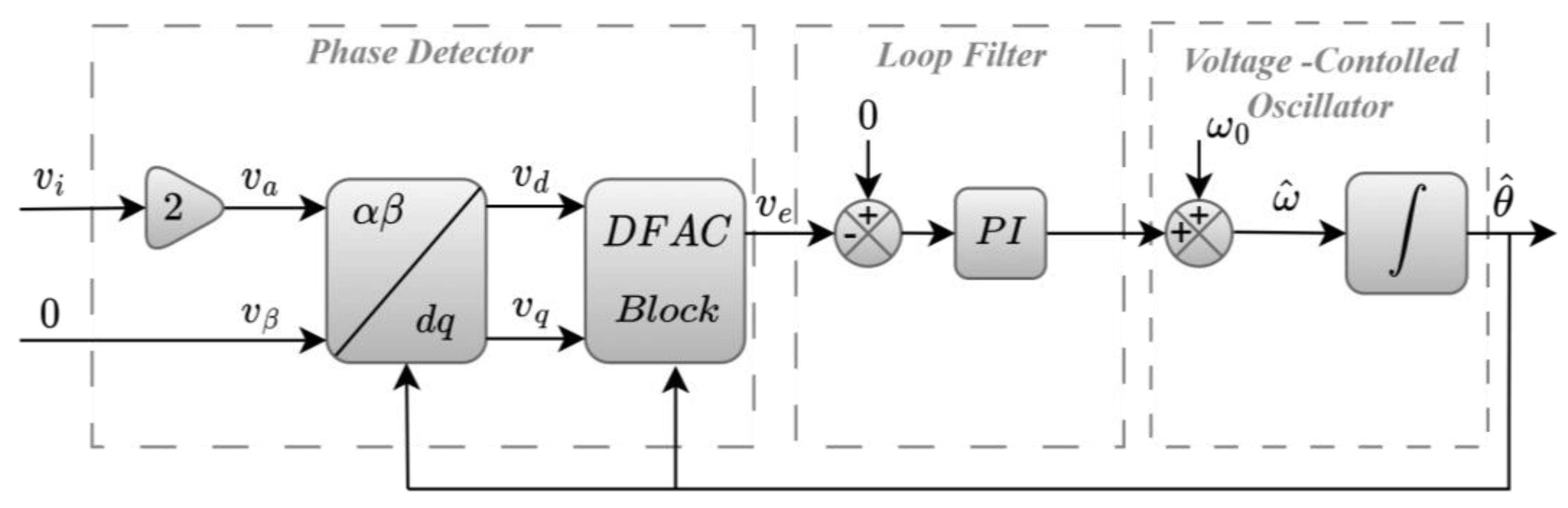
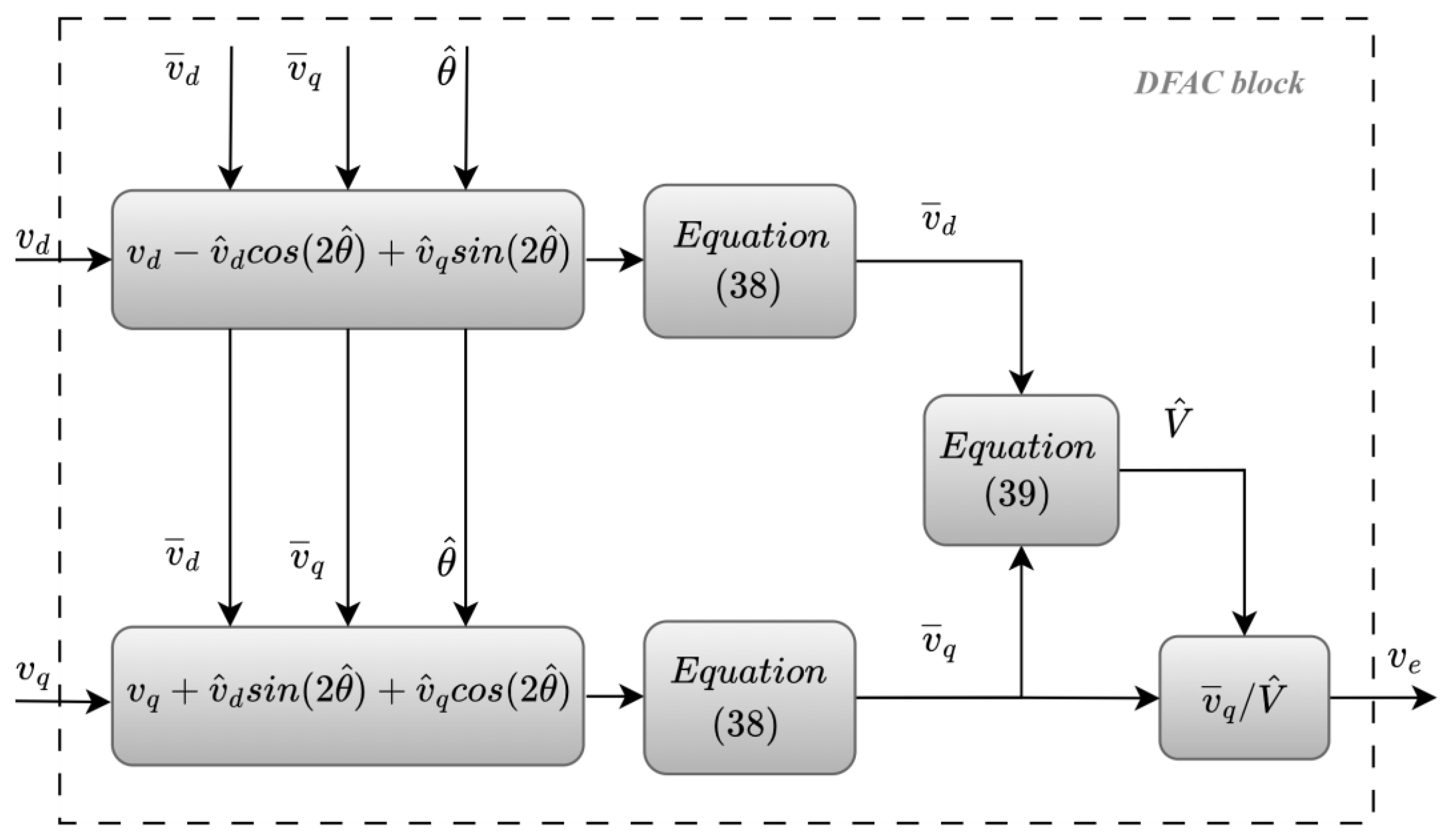
4.3. Double Frequency and Amplitude Compensation (DFAC)-PLL-Based Algorithm for Single-Phase Synchrophasor Estimation

The authors in [41] investigated the compliance of the single-phase EPLL [2] and DFAC-PLL [42] with the IEEE standard [7] for M-class PMU without considering the pre-filtering and post-filtering stages. In this section, the single-phase EPLL is not discussed due to the previous analysis of the three-phase EPLL in Section 4.2. The basic structure of DFAC-PLL consists of two blocks, namely, the αβ-dq block and DFAC block depicted in Figure 7. The single-phase signal $v_i\left(t\right)=Vcos\left(\omega t+\phi \right)$ is transformed into rotation reference frame $v_d\left(t\right)$, $v_q\left(t\right)$ using the Park Transformation in Equation (35):

$$\left[\begin{array}{c}{v}_d\left(t\right)\\ v_q\left(t\right)\end{array}\right]=\left[\begin{array}{cc}cos\left(\hat{\theta }\right)& sin\left(\hat{\theta }\right)\\ -sin\left(\hat{\theta }\right)& cos\left(\hat{\theta }\right)\end{array}\right]\left[\begin{array}{c}2v_i\left(t\right)\\ 0\end{array}\right]=V\left[\begin{array}{c}cos\left(\theta -\hat{\theta }\right)+cos\left(\theta +\hat{\theta }\right)\\ sin\left(\theta -\hat{\theta }\right)-sin\left(\theta +\hat{\theta }\right)\end{array}\right]$$

(35)

where $V$ is the amplitude of the input cosine function signal, $\theta =\omega t+\phi$, $\omega$ is the angular frequency of the power network, $\hat{\theta }$ is the estimated phase angle and $\phi$ is the initial phase angle at time zero. Considering ${\theta }_e=\theta -\hat{\theta }$, Equation (35) can be written as in Equations (36) and (37).

$$v_d\left(t\right)=Vcos\left({\theta }_e\right)+Vcos\left({\theta }_e\right)\mathit{cos}\left(2\hat{\theta }\right)-Vsin\left({\theta }_e\right)\mathit{sin}\left(2\hat{\theta }\right)$$

(36)

$$v_q\left(t\right)=Vsin\left({\theta }_e\right)-Vsin\left({\theta }_e\right)\mathit{cos}\left(2\hat{\theta }\right)-Vcos\left({\theta }_e\right)\mathit{sin}\left(2\hat{\theta }\right)$$

(37)

In case the PLL is locked, meaning that the estimated angle is very close to the corresponding actual angle, ${\theta }_e$ becomes very small, and the terms $Vcos\left({\theta }_e\right)$ and $Vsin\left({\theta }_e\right)$ of Equations (36) and (37) can be considered almost dc components. Additionally, it is observed that the amplitudes of the trigonometric functions running at twice the nominal frequency rely on these dc components. The authors in [42] proposed a method to eliminate these undesired double-frequency components by generating the same signals in order to subtract them from the $v_d$ and $v_q$ components, as depicted in Figure 8. The DFAC structure comprises a double-frequency elimination block and an amplitude compensation block. The LPF block is considered as a first-order low-pass filter as shown in Equation (38):

$$LPF\left(s\right)=\frac{{\omega }_p}{s+{\omega }_p}$$

(38)

where ${\omega }_p$ is the cut-off frequency of the LPF. Moreover, the estimated amplitude of the input signal is derived from the filtered values of the dq components as in Equation (39).

$$\hat{V}=\sqrt{{\overline{v}}_d^2+{\overline{v}}_q^2}$$

(39)

The proposed PLL presents satisfactory compensation for the unwanted double-frequency oscillations, as well as the input signal amplitude fluctuations, while providing a fast dynamic response. Furthermore, it provides high rejection capability in the presence of disturbances, as well as stable and reliable performance.

4.3.1. Simulation Results under Steady-State Conditions

In this section, the simulation results for the steady-state conditions of M-class PMU performed by the authors in [41] are summarized. The reporting rate is considered 100 FPS.

• Amplitude step change test: The amplitude of the input signal applied to the PLL varies from 10% to 120% in steps of 10% of the nominal amplitude. The limits for FE, RFE and TVE defined in IEEE standard [4,7] are 0.005 Hz, 0.1 Hz/s and 1%, respectively. The corresponding estimated values provided by the PLL meet the requirements.
• Phase angle step change test: The phase angle of the input signal applied to the PLL varies from −180° to 180°. The error limits are the same as the amplitude step test. The error values FE, RFE and TVE provided by the PLL comply with the IEEE standard [4,7].
• Frequency step change test: The frequency of the input signal applied to the PLL varies from 45 to 55 Hz. The limits for FE, RFE and TVE are the same as the amplitude step test. The corresponding estimated values, provided by the PLL, meet the requirements.
• Harmonics distortion test: Different sinusoidal signals containing harmonics (from 2nd to 50th) one at a time with an amplitude of 10% are applied to the PLL. The limits for FE and TVE defined in IEEE standard [4,7] are 0.025 Hz and 1%, respectively. The PLL provides TVE and FE within limits for harmonic orders greater than 10th and 39th, respectively.
• Out-of-band interference test: Different sinusoidal signals with frequency range 10–44 Hz and 56–100 Hz in steps of 1 Hz having 10% of nominal amplitude are applied to the PLL. The proposed PLL failed to comply with the IEEE standard [4,7].

4.3.2. Simulation Results under Dynamic Conditions

In this section, the simulation results for the dynamic conditions of M-class PMU performed by the authors in [41] are summarized. The reporting rate is considered 100 FPS.

• Amplitude and phase angle modulation test: A sinusoidal modulation in the amplitude (with modulation frequency varying from 0.1 to 5 Hz) with a magnitude of 10% is applied to the PLL. According to the IEEE standard [4,7], the limits for FE, RFE and TVE are 0.3 Hz, 14 Hz/s and 3%, respectively. The proposed PLL succeeds in complying with the Standard for the FE and TVE but violates the RFE limit.
• Linear frequency ramp test: The frequency of the grid voltages increases with a ramp function of 1 Hz/s. Under this dynamic condition, the PLL complies with the IEEE standard [4,7].
• Amplitude and phase angle step change test: The purpose of this test is to determine the time response of the algorithm in the step change of the amplitude and phase angle. In this test, the DFAC-PLL violates the requirements of the IEEE standard [4,7].

It should be mentioned that the above tests for steady-state and dynamic conditions were performed without the use of pre- and post-filtering stages.

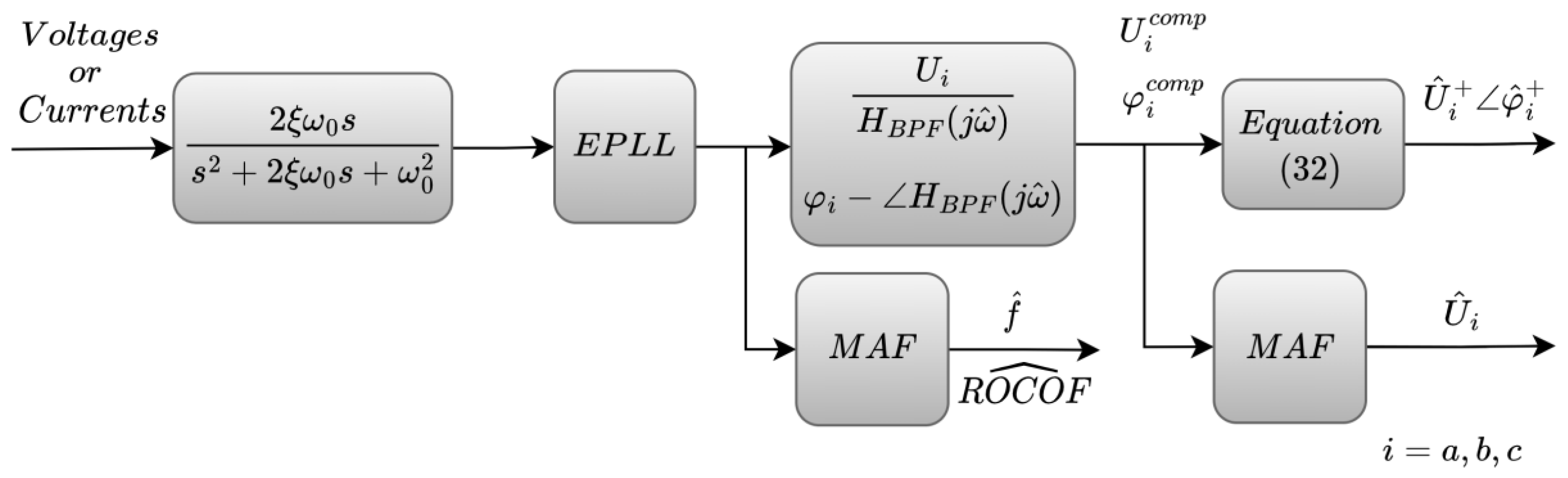
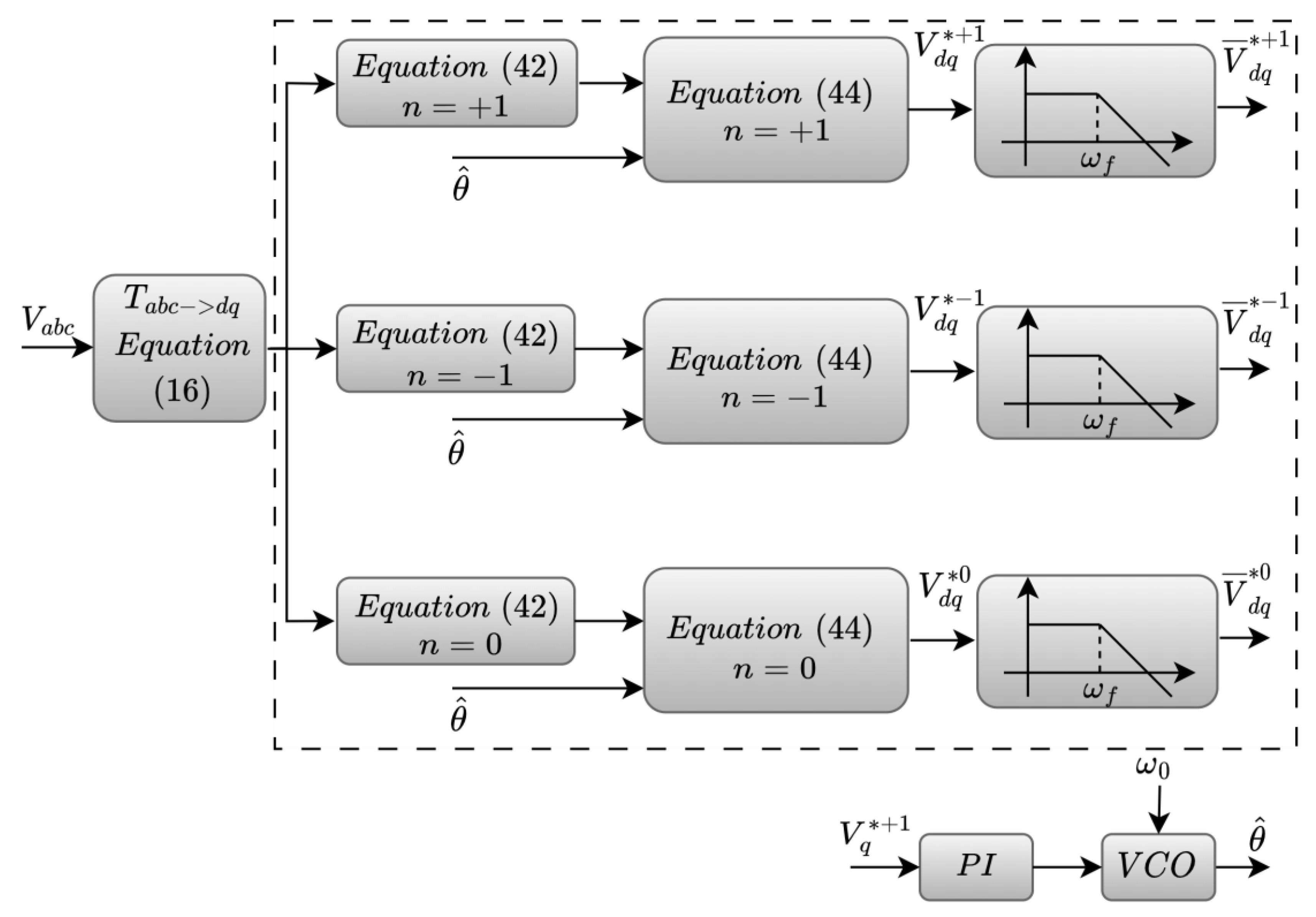
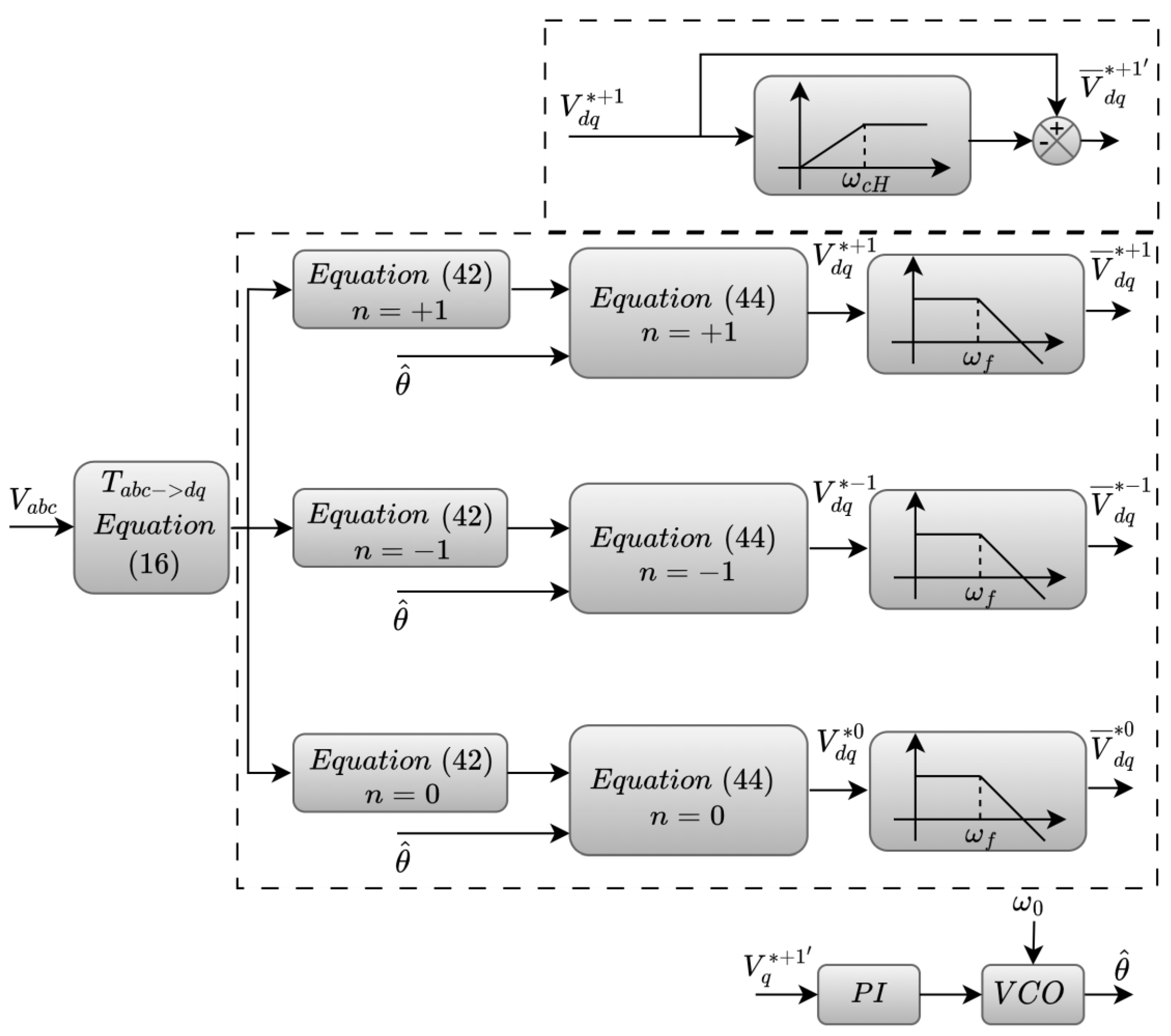
4.4. Harmonic Inter-Harmonic and DC Offset (HIHDO)-PLL-Based Algorithm for Three-Phase System Synchrophasor Estimation

The authors in [43] explore by testing the performance of four types of PLL techniques to find the most suitable candidate for PMU algorithm implementation, namely, the SRF-PLL, Decoupling Network Alpha-Beta (DNαβ)-PLL, Harmonic Inter-harmonic and DC Offset (HIHDO)-PLL and Alpha-Beta Enhanced Prefiltering Moving Average (αβEPMAF)-PLL. In this section, the HIHDO-PLL [44] is presented since it shows satisfactory experimental results in order to be employed for PMU development [43].

The proposed PLL in [44] considers the effect of harmonics, inter-harmonics and DC-offset components in the grid voltage while estimating the grid voltage by using decoupling network cells (DCs). The three-phase grid signals ${\mathit{v}}_{abc}$ transformed into dq frame ${\mathit{v}}_{dq}$ can be expressed as in Equation (40):

$${\mathit{v}}_{dq}={\mathit{v}}_{dq}^{+1}+{\mathit{v}}_{dq}^{-1}+{\mathit{v}}_{dq}^0+\sum v_{dq}^h$$

(40)

where ${\mathit{v}}_{dq}^{+1}$, ${\mathit{v}}_{dq}^{-1}$ and ${\mathit{v}}_{dq}^0$ are the positive-sequence, negative-sequence and DC offset components in the rotating reference frame, respectively, while $\sum {\mathit{v}}_{dq}^h$ is the sum of the remaining harmonic and inter-harmonic components that appear in the dq-frame due to the network’s abnormal conditions. The transformation of the three-phase signals into a dq-frame is performed using Equation (41). Under normal grid conditions, the transformation of the three-phase input signals ${\mathit{v}}_{abc}$ presented in Equation (41) leads to only a positive-sequence component, which in principle is a dc component without any oscillation term. However, in case of abnormal grid conditions, the dq components contain the undesired oscillation term because of the negative-sequence component, the DC-offset component, and the remaining harmonic and inter-harmonic components of the grid distortion depicted in Equation (41):

$${\mathit{v}}_{dq}^n=V^n\left[\begin{array}{c}cos\left({\theta }_n\right)\\ sin\left({\theta }_n\right)\end{array}\right]+{\displaystyle \sum }_{n\ne m}\left\{V^m\left[T_{dq}^{n-m}\right]\left[\begin{array}{c}cos\left({\theta }_m\right)\\ sin\left({\theta }_m\right)\end{array}\right]\right\}$$

(41)

where the Park transformation matrix is shown in Equation (42).

$$\left[T_{dq}^n\right]=\left[\begin{array}{cc}cos\left(nwt\right)& sin\left(nwt\right)\\ -sin\left(nwt\right)& cos\left(nwt\right)\end{array}\right]$$

(42)

The oscillation term, rotating at the angular speed of $nwt$, and the dc term caused by the abnormal conditions of the grid are observed in Equation (41). This oscillation term results in inaccurate computation of the amplitude and phase angle of the positive-sequence component and must be removed.

In Figure 9, the cells that eliminate the presence of the negative-sequence component and DC-offset component without considering the presence of harmonic and inter-harmonic components are presented. This kind of PLL is also known as DC-offset compensation cell (DOCC)-PLL.

For $n=+1,-1$ and 0, Equation (41) can be written as in Equation (43). Rearranging Equation (43) and substituting vector ${\mathit{V}}_{dq}^n$ with the filtered estimated dc-component vector ${\overline{\mathit{V}}}_{dq}^{\ast n}$ used for the feedback terms, Equation (44) is acquired, where the LPF for the mitigation of the high-frequency components is depicted in Equation (45), and ${\omega }_f$ denotes the cut-off frequency of the filter. The decoupled filtered positive sequence of the q-component is used in the final stage of the PLL for phase tracking.

$$\left[\begin{array}{c}{\mathit{v}}_{dq}^{+1}\\ {\mathit{v}}_{dq}^{-1}\\ {\mathit{v}}_{dq}^0\end{array}\right]=\left[\begin{array}{c}{\mathit{V}}_{dq}^{+1}\\ {\mathit{V}}_{dq}^{-1}\\ {\mathit{V}}_{dq}^0\end{array}\right]+\left[\begin{array}{ccc}\left[0\right]& T_{dq}^{+1-\left(-1\right)}& T_{dq}^{+1-\left(0\right)}\\ T_{dq}^{-1-\left(+1\right)}& \left[0\right]& T_{dq}^{-1-\left(0\right)}\\ T_{dq}^{0-\left(+1\right)}& T_{dq}^{0-\left(-1\right)}& \left[0\right]\end{array}\right]\left[\begin{array}{c}{\mathit{V}}_{dq}^{+1}\\ {\mathit{V}}_{dq}^{-1}\\ {\mathit{V}}_{dq}^0\end{array}\right]$$

(43)

$$\left[\begin{array}{c}{\mathit{V}}_{dq}^{\ast +1}\\ {\mathit{V}}_{dq}^{\ast -1}\\ {\mathit{V}}_{dq}^{\ast 0}\end{array}\right]=\left[\left[\begin{array}{c}{\mathit{v}}_{dq}^{+1}\\ {\mathit{v}}_{dq}^{-1}\\ {\mathit{v}}_{dq}^0\end{array}\right]-\left[\begin{array}{ccc}\left[0\right]& T_{dq}^{+1-\left(-1\right)}& T_{dq}^{+1-\left(0\right)}\\ T_{dq}^{-1-\left(+1\right)}& \left[0\right]& T_{dq}^{-1-\left(0\right)}\\ T_{dq}^{0-\left(+1\right)}& T_{dq}^{0-\left(-1\right)}& \left[0\right]\end{array}\right]\left[\begin{array}{c}{\overline{\mathit{V}}}_{dq}^{\ast +1}\\ {\overline{\mathit{V}}}_{dq}^{\ast -1}\\ {\overline{\mathit{V}}}_{dq}^{\ast 0}\end{array}\right]\right]$$

(44)

$$\left[F\left(s\right)\right]=LPF\left(s\right)=\frac{{\omega }_f}{s+{\omega }_f}\left[\begin{array}{cc}1& 0\\ 0& 1\end{array}\right]$$

(45)

The effects of harmonic and inter-harmonic imposed on the grid are faced by adding a distinctive harmonic compensation network cell (HCN) in the existing DOCC-PLL. This addition constitutes the HIHDO-PLL, proposed in [44]. Figure 10 depicts the HIHDO-PLL block structure.

The transfer functions of the harmonic compensation network cell of the dq- and αβ-domain are presented in Equations (46) and (47), respectively, while the overall transfer function of the proposed method is shown in Equation (48).

$$F_{HCN}\left(s\right)=\frac{{\mathit{V}}_{dq}^{\ast +1^{\prime }}}{{\mathit{V}}_{dq}^{\ast +1}}=1-\frac{s}{s+{\omega }_{cH}}$$

(46)

$$T_{HCN}\left(s\right)=\frac{{\mathit{V}}_{\alpha \beta }^{\ast +1^{\prime }}}{{\mathit{V}}_{\alpha \beta }^{\ast +1}}=1-\frac{s-j\omega }{s+({\omega }_{cH}-j\omega )}$$

(47)

$$H_{HIHDO}\left(s\right)=\left[1-\frac{s-j\omega }{s+({\omega }_{cH}-j\omega )}\right]\left\{\frac{1-\left[TF{T}^{-1}+TF{T}^0\right]}{1-\left[TF{T}^{-1}+TF{T}^0\right]TF{T}^{+1}}\right\}$$

(48)

where ${\omega }_{cH}$ is the cut-off frequency of the high-pass filter (HPF) and $T^n$ and $F$ are expressed in Equations (42) and (45), respectively. The decoupled filtered (from the oscillation term) positive sequence of the q-component is used in the final stage of the PLL for phase tracking. In case the PLL is locked, meaning that ${\overline{\mathit{V}}}_q^{\ast +1^{\prime }}=0$, the estimated positive-sequence phase amplitude and angle, as well as frequency, are obtained from the final stage of the PLL, ${\overline{\mathit{V}}}_d^{\ast +1^{\prime }}$, $\hat{\theta }$ and $\hat{\omega }/2\pi$, respectively.

4.4.1. Simulation Results of the HIHDO PLL-Based PMU Algorithm

The HIHDO PLL-based PMU algorithm first undergoes a phase angle jump of +30°, followed by a grid unbalanced fault. The PLL presents a fast dynamic response, about 50 ms, for estimating the frequency and phase angle of the three-phase input signal, whereas it provides a small delay for estimating the corresponding amplitude. Then, the three-phase input signal of the PLL was distorted by adding 5% of the 7th harmonic and 6% of DC offset. The simulation results showed that the proposed PLL mitigates the undesired oscillations caused by the abnormal grid conditions, without sacrificing the accuracy of the measured values.

4.4.2. Experimental Results of the HIHDO PLL-Based PMU Algorithm

In this section, the numerical results of the experimental testing of the HIHDO PLL-based PMU conducted in [43] are summarized. The following tests have been performed:

• Phase angle step change test: The three-phase input signals undergo a phase angle jump of +30°. The PMU managed to track the phase angle step change while it obtained the value of +30° in 70 ms. During transients, slight overshoots occurred in the waveforms of the estimated signal amplitude and frequency with a settling time of 80 ms. Under this condition, the frequency reached 2.1 Hz and the amplitude 0.1 per unit at the time the phase angle step change occurred.
• Harmonic distortion test: In the grid voltages, the following harmonics were injected: 5th and 7th with the corresponding amplitude of 6% and 5% of the fundamental component. Furthermore, a phase angle step of −20° was introduced. The PMU succeeded in rejecting the high-frequency components while accurately estimating the signal amplitude, angle and frequency. During the transients, the voltage amplitude and frequency overshot were 1.6 Hz and 0.05 per unit, respectively. The settling times for the frequency, magnitude and phase estimations were 80 ms, 66 ms and 65 ms, respectively.
• Inter-harmonics and DC-offset rejection test: The PMU succeeded in rejecting the inter-harmonic and DC-offset components while accurately estimating the voltage amplitude, phase angle and frequency.
• Harmonics and voltage sag injection, and frequency step test: A combined set of test signals were applied to the proposed PLL-based PMU, comprising of 5% 7th, 3.5% 11th, 3% 15th and 2% 17th harmonics, voltage sag of 37% and frequency step change of −2 Hz. The harmonics were effectively compensated, resulting in an accurate estimation of voltage amplitude, phase angle and frequency. The proposed algorithm managed to detect the voltage sag within 10 ms while the settling time for the estimated frequency and phase angle were 80 ms and 140 ms, respectively. Furthermore, the PMU tracked the step change of the frequency within 100 ms.

5. Discussion

Based on extensive mathematical analysis and numerical results of experiments and simulations with various PLL-based PMU methods presented in the recent literature, a summary of the challenges to be addressed are discussed, while possible research extensions in the field of PMU algorithms are suggested.

• The PID SRF-PLL-based PMU algorithm provides satisfactory experimental results in the estimation of positive-sequence amplitude, phase angle, frequency and ROCOF. In addition, the implementation of the algorithm presents a low computational burden, making it capable of being developed on a general-purpose microcontroller with DSP features. The experimental results showed that the proposed PLL-based PMU algorithm for the synchrophasor estimation complies with all the IEEE standard requirements [4,7] for both PMU classes P and M, while in conjunction with the low computational cost, makes it attractive for implementation of low-cost PMUs in order to be used in distribution networks [35], although it provides a low reporting rate.
• The EPLL-based PMU algorithm provides good experimental and simulation results in estimating positive-sequence amplitude, phase angle, frequency and ROCOF for a P-class PMU. It is worth noting that the estimated frequency and ROCOF are derived from the processing of the information obtained from all three signal components, making these estimated measurements more reliable and stable. In terms of amplitude and phase angle modulation tests, the proposed method meets TVE requirements but failed in estimating accurately the frequency as well as the ramp frequency test [21]. The proposed PMU algorithm addresses the abnormal grid conditions such as imbalances and harmonics, while also providing a fast dynamic response and acceptable steady-state accuracy which make it a potential candidate algorithm for a P-class phasor measurement unit [39]. It can be observed from [39] that the computational complexity of the proposed algorithm is low; therefore, it can be implemented on a low-cost microprocessor.
• The DFAC-PLL is a single-phase PLL that can estimate the phase amplitude, angle and frequency of the input signal [42]. Although the compliance testing of the PLL in accordance with the IEEE standard [4,7] is performed without the pre- and post-filtering stages, it shows that it can meet the requirements of the steady-state condition tests, while exceeding the acceptable limits in the harmonic distortion and out-of-band interference tests. In terms of dynamic condition tests, the proposed PLL meets the requirements for the synchrophasor estimation when subjected to the amplitude modulation test but exceeded the limitations in the phase angle modulation test. In case the DFAC-PLL is to be used for synchrophasor estimation algorithm, the filtering and compensation stages are required.
• The HIHDO-PLL-based PMU successfully faces the normal and abnormal grid conditions, while presenting excellent simulation results in the estimation of the positive-sequence component of phase magnitude and angle of the power grid. Moreover, it provides fast dynamic response and slight overshoots without sacrificing the required accuracy under harmonically polluted and faulty network conditions which is also the case for the estimation of the synchrophasor in a more realistic power grid. The proposed PLL presents a lower computational burden compared with existing PLL algorithms in the recent literature for addressing both the imbalances and harmonic distortion due to abnormal grid conditions, but its execution requires 106 mathematical operations, which is an important burden if its implementation is performed by a general-purpose microcontroller with DSP features. With the exception of the computational burden, the mathematical analysis and simulation results on network faults showed that the HIHDO-PLL has the potential to be used for synchrophasor estimation algorithms [43].

The performance of the discussed PLL-based PMU algorithms is summarized in

Table 1. Performance summary of PLL-based PMU methods.

	PLL-Based PMU Approach
	PID SRF-PLL	EPLL	DFAC-PLL	HIHDO-PLL
Harmonic rejection	Good	Good	Poor	Very good
Dynamic response	Faster	Fast	Slow	Fast
Computational burden	Low	Medium	Medium	High
Compliant with IEEE Std.	Yes, for P and M classes	Yes, for P class. Minor deviations	No	Should be investigated

.

6. Conclusions

In this literature review, various PLL-based PMUs have been extensively analyzed through mathematical analysis by providing numerical results of experimental and simulation tests according to their measurement applicability, for addressing the major challenges of synchrophasor estimation under normal and abnormal grid conditions. Overall, PLL algorithms are widespread in the field of power electronics converters connected to the utility network owing to their fast dynamic response, good tracking of frequency and phase angle and estimation quality. Exploiting their existing technological maturity as well as their flexibility and adaptability of the implementation makes them attractive and suitable candidates for reliable and low-cost PMUs. The SRF-based PLL, including their modifications such as decoupling cells for the harmonic and inter-harmonic rejection, proves to be most suitable for developing synchrophasor estimation algorithms, while providing fast response and accuracy under non-ideal grid conditions. The main topics that should be further investigated in future PLL-based PMU implementations focus on accuracy, computational efficiency, response under dynamic conditions as well as harmonic and inter-harmonic rejection capability.

References

1. Monti, A.; Muscas, C.; Ponci, F. (Eds.) Phasor Measurement Units and Wide Area Monitoring Systems: From the Sensors to the System; Elsevier: Amsterdam, The Netherlands, 2016; ISBN 978-0-12-804569-5. [Google Scholar]
2. Karimi-Ghartemani, M.; Ooi, B.-T.; Bakhshai, A. Application of Enhanced Phase-Locked Loop System to the Computation of Synchrophasors. IEEE Trans. Power Deliv. 2011, 26, 22–32. [Google Scholar] [CrossRef]
3. Talukder, Z.; Nishat Tasnim, K.; Reza, M.S. A Comparative Study of Various Methods of Phasor Measurement Unit Algorithms. In Proceedings of the 2019 1st International Conference on Advances in Science, Engineering and Robotics Technology (ICASERT), Dhaka, Bangladesh, 3–5 May 2019; pp. 1–6. [Google Scholar]
4. IEEE Std C37.118.1-2011; IEEE Standard for Synchrophasor Measurements for Power Systems. IEEE: Piscateville, NJ, USA, 2011.
5. IEEE Std C37.118-2005 (Revision of IEEE Std 1344-1995); IEEE Standard for Synchrophasors for Power Systems. IEEE: Piscateville, NJ, USA, 2006; pp. 1–65.
6. IEEE Std C37.118.1a-2014 (Amendment to IEEE Std C37.118.1-2011); IEEE Standard for Synchrophasor Measurements for Power Systems Amendment 1: Modification of Selected Performance Requirements. IEEE: Piscataway, NJ, USA, 2014.
7. IEEE Std C37.118.2-2011; IEEE Standard for Synchrophasor Data Transfer for Power Systems. IEEE: Piscataway, NJ, USA, 2011.
8. Karimi-Ghartemani, M.; Ooi, B.-T.; Bakhshai, A. Investigation of DFT-Based Phasor Measurement Algorithm. In Proceedings of the IEEE PES General Meeting, Providence, RI, USA, 25–29 July 2010; pp. 1–6. [Google Scholar]
9. Zhan, L.; Liu, Y.; Liu, Y. A Clarke Transformation-Based DFT Phasor and Frequency Algorithm for Wide Frequency Range. IEEE Trans. Smart Grid 2018, 9, 67–77. [Google Scholar] [CrossRef]
10. Derviškadić, A.; Romano, P.; Paolone, M. Iterative-Interpolated DFT for Synchrophasor Estimation in M-Class Compliant PMUs. In Proceedings of the 2017 IEEE Manchester PowerTech, Manchester, UK, 18–22 June 2017; pp. 1–6. [Google Scholar]
11. Romano, P.; Paolone, M. Enhanced Interpolated-DFT for Synchrophasor Estimation in FPGAs: Theory, Implementation, and Validation of a PMU Prototype. IEEE Trans. Instrum. Meas. 2014, 63, 2824–2836. [Google Scholar] [CrossRef]
12. Romano, P.; Paolone, M. An Enhanced Interpolated-Modulated Sliding DFT for High Reporting Rate PMUs. In Proceedings of the 2014 IEEE International Workshop on Applied Measurements for Power Systems Proceedings (AMPS), Aachen, Germany, 24–26 September 2014; pp. 1–6. [Google Scholar]
13. De la O Serna, J.A.; Rodriguez-Maldonado, J. Instantaneous Oscillating Phasor Estimates with TaylorK-Kalman Filters. IEEE Trans. Power Syst. 2011, 26, 2336–2344. [Google Scholar] [CrossRef]
14. Dash, P.K.; Hasan, S. A Fast Recursive Algorithm for the Estimation of Frequency, Amplitude, and Phase of Noisy Sinusoid. IEEE Trans. Ind. Electron. 2011, 58, 4847–4856. [Google Scholar] [CrossRef]
15. Platas-Garza, M.A.; de La O Serna, J.A. Dynamic Phasor and Frequency Estimates through Maximally Flat Differentiators. IEEE Trans. Instrum. Meas. 2010, 59, 1803–1811. [Google Scholar] [CrossRef]
16. Roscoe, A.J.; Abdulhadi, I.F.; Burt, G.M. P and M Class Phasor Measurement Unit Algorithms Using Adaptive Cascaded Filters. IEEE Trans. Power Deliv. 2013, 28, 1447–1459. [Google Scholar] [CrossRef] [Green Version]
17. De La O Serna, J.A. Synchrophasor Measurement with Polynomial Phase-Locked-Loop Taylor–Fourier Filters. IEEE Trans. Instrum. Meas. 2015, 64, 328–337. [Google Scholar] [CrossRef]
18. Castello, P.; Liu, J.; Muscas, C.; Pegoraro, P.A.; Ponci, F.; Monti, A. A Fast and Accurate PMU Algorithm for P+M Class Measurement of Synchrophasor and Frequency. IEEE Trans. Instrum. Meas. 2014, 63, 2837–2845. [Google Scholar] [CrossRef]
19. Toscani, S.; Muscas, C.; Pegoraro, P.A. Design and Performance Prediction of Space Vector-Based PMU Algorithms. IEEE Trans. Instrum. Meas. 2017, 66, 394–404. [Google Scholar] [CrossRef]
20. Toscani, S.; Muscas, A. Space Vector Based Approach for Synchrophasor Measurement. In Proceedings of the 2014 IEEE International Instrumentation and Measurement Technology Conference (I2MTC) Proceedings, Montevideo, Uruguay, 12–15 May 2014; pp. 257–261. [Google Scholar]
21. Karimi-Ghartemani, M.; Mojiri, M.; Bakhshai, A.; Jain, P. A Phasor Measurement Algorithm Based on Phase-Locked Loop. In Proceedings of the PES T&D 2012, Orlando, FL, USA, 7–10 May 2012; pp. 1–6. [Google Scholar]
22. Sun, K.; Zhou, Q.; Liu, Y. A Phase Locked Loop-Based Approach to Real-Time Modal Analysis on Synchrophasor Measurements. IEEE Trans. Smart Grid 2014, 5, 260–269. [Google Scholar] [CrossRef]
23. Messina, F.; Marchi, P.; Rey Vega, L.; Galarza, G.; Laiz, H. A Novel Modular Positive-Sequence Synchrophasor Estimation Algorithm for PMUs. IEEE Trans. Instrum. Meas. 2017, 66, 1164–1175. [Google Scholar] [CrossRef]
24. Ferrero, R.; Pegoraro, P.A.; Toscani, S. A Space Vector Phase-Locked-Loop Approach to Synchrophasor, Frequency and Rocof Estimation. In Proceedings of the 2019 IEEE International Instrumentation and Measurement Technology Conference (I2MTC), Auckland, New Zealand, 20–23 May 2019; pp. 1–6. [Google Scholar]
25. Ferrero, R.; Pegoraro, P.A.; Toscani, S. Proposals and Analysis of Space Vector-Based Phase-Locked-Loop Techniques for Synchrophasor, Frequency, and ROCOF Measurements. IEEE Trans. Instrum. Meas. 2020, 69, 2345–2354. [Google Scholar] [CrossRef]
26. Trento, B.; Wang, B.; Sun, K.; Tolbert, L.M. Integration of Phase-Locked Loop Based Real-Time Oscillation Tracking in Grid Synchronized Systems. In Proceedings of the 2014 IEEE PES General Meeting|Conference & Exposition, Washington, DC, USA, 27–31 July 2014; pp. 1–5. [Google Scholar]
27. De Carvalho, G.U.; Weber Denardin, G.; Cardoso, R.; Moraes, F. Design and Test of a SRF-PLL Based Algorithm for Positive-Sequence Synchrophasor Measurements. In Proceedings of the 2019 IEEE 15th Brazilian Power Electronics Conference and 5th IEEE Southern Power Electronics Conference (COBEP/SPEC), Santos, Brazil, 1–4 December 2019; pp. 1–6. [Google Scholar]
28. Golestan, S.; Guerrero, J.M.; Vasquez, J. Three-Phase PLLs: A Review of Recent Advances. IEEE Trans. Power Electron. 2017, 32, 1894–1907. [Google Scholar] [CrossRef] [Green Version]
29. Santos Filho, M.; Seixas, P.F.; Cortizo, P.; Torres, L.A.B.; Souza, A.F. Comparison of Three Single-Phase PLL Algorithms for UPS Applications. IEEE Trans. Ind. Electron. 2008, 55, 2923–2932. [Google Scholar] [CrossRef]
30. Karimi-Ghartemani, M.; Iravani, M. A Method for Synchronization of Power Electronic Converters in Polluted and Variable-Frequency Environments. IEEE Trans. Power Syst. 2004, 19, 1263–1270. [Google Scholar] [CrossRef]
31. Chung, S.-K. A Phase Tracking System for Three Phase Utility Interface Inverters. IEEE Trans. Power Electron. 2000, 15, 431–438. [Google Scholar] [CrossRef] [Green Version]
32. Velasco, D.; Trujillo, C.; Garcera, G.; Figueres, E. An Active Anti-Islanding Method Based on Phase-PLL Perturbation. IEEE Trans. Power Electron. 2011, 26, 1056–1066. [Google Scholar] [CrossRef] [Green Version]
33. Kaura, V.; Blasko, V. Operation of a Phase Locked Loop System under Distorted Utility Conditions. IEEE Trans. Ind. Appl. 1997, 33, 58–63. [Google Scholar] [CrossRef]
34. Liu, B.; Zhuo, F.; Zhu, Y.; Yi, H.; Wang, F. A Three-Phase PLL Algorithm Based on Signal Reforming Under Distorted Grid Conditions. IEEE Trans. Power Electron. 2015, 30, 5272–5283. [Google Scholar] [CrossRef]
35. De Carvalho, G.U.; Denardin, G.W.; Cardoso, R.; Grando, F.L. A PID SRF-PLL Based Algorithm for Positive-sequence Synchrophasor Measurements. Int. Trans. Electr. Energy Syst. 2021, 31, e12777. [Google Scholar] [CrossRef]
36. Fortescue, L. Method of Symmetrical Co-Ordinates Applied to the Solution of Polyphase Networks. Trans. Am. Inst. Electr. Eng. 1918, XXXVII, 1027–1140. [Google Scholar] [CrossRef]
37. Rodriguez, P.; Pou, J.; Bergas, J.; Candela, J.I.; Burgos, P.; Boroyevich, D. Decoupled Double Synchronous Reference Frame PLL for Power Converters Control. IEEE Trans. Power Electron. 2007, 22, 584–592. [Google Scholar] [CrossRef]
38. Karimi-Ghartemani, M.; Mojiri, M.; Safaee, A.; Walseth, J.A.; Khajehoddin, S.A.; Jain, P.; Bakhshai, A. A New Phase-Locked Loop System for Three-Phase Applications. IEEE Trans. Power Electron. 2013, 28, 1208–1218. [Google Scholar] [CrossRef]
39. Costa, T.B.; Berriel, O.; Lima, A.S.; Dias, F.S. Evaluation of a Phase-Locked Loop Phasor Measurement Algorithm on a Harmonic Polluted Environment in Applications Such as PMU. J. Control Autom. Electr. Syst. 2019, 30, 424–433. [Google Scholar] [CrossRef]
40. Kundur, P. Power System Stability and Control; McGraw-Hill Professional: New York, NY, USA, 1994. [Google Scholar]
41. Kumar, P.; Gurrala, G. IEEE C37.118.1a-2014 Compliance Testing of EPLL and DFAC-PLL for Synchrophasors. In Proceedings of the 2018 North American Power Symposium (NAPS), Fargo, ND, USA, 9–11 September 2018; pp. 1–6. [Google Scholar]
42. Golestan, S.; Monfared, M.; Freijedo, F.D.; Guerrero, J.M. Design and Tuning of a Modified Power-Based PLL for Single-Phase Grid-Connected Power Conditioning Systems. IEEE Trans. Power Electron. 2012, 27, 3639–3650. [Google Scholar] [CrossRef] [Green Version]
43. Ali, Z.; Saleem, K.; Brown, R.; Christofides, N.; Dudley, S. Performance Analysis and Benchmarking of PLL-Driven Phasor Measurement Units for Renewable Energy Systems. Energies 2022, 15, 1867. [Google Scholar] [CrossRef]
44. Ali, Z.; Christofides, N.; Hadjidemetriou, L.; Kyriakides, E. Design of an Advanced PLL for Accurate Phase Angle Extraction under Grid Voltage HIHs and DC Offset. IET Power Electron. 2018, 11, 995–1008. [Google Scholar] [CrossRef]
Figure 1. Block diagram of the single-phase PLL.
Energies 16 05465 g001
Figure 2. Convention for synchrophasor representation.
Energies 16 05465 g002
Figure 3. Block diagram of the three-phase SRF-PLL.
Energies 16 05465 g003
Figure 4. Block diagram of the SRF-PLL-based algorithm for positive-sequence synchrophasor estimation.
Energies 16 05465 g004
Figure 5. Block structure of the EPLL.
Energies 16 05465 g005
Figure 6. Block structure of the EPLL-based phasor measurement.
Energies 16 05465 g006
Figure 7. Basic block diagram of DFAC-PLL.
Energies 16 05465 g007
Figure 8. Block diagram of DFAC.
Energies 16 05465 g008
Figure 9. The block diagram of DOCC-PLL.
Energies 16 05465 g009
Figure 10. The block diagram of the HIHDO-PLL.
Energies 16 05465 g010