Article

Machine Learning Estimation of Battery Efficiency and Related Key Performance Indicators in Smart Energy Systems

1
Department of Electronic Technology, University of Seville, 41004 Seville, Spain
2
Chair of Electrical Energy Storage Technology, Department of Energy and Process Engineering, TUM School of Engineering and Design, Technical University of Munich (TUM), 80333 Munich, Germany
3
Department of Mechanical Engineering, Institute for Energy and Propulsion Technologies (IEAT), Kempten University of Applied Sciences, 87435 Kempten, Germany
*
Author to whom correspondence should be addressed.
Energies 2023, 16(14), 5548; https://doi.org/10.3390/en16145548
Submission received: 21 June 2023 / Revised: 16 July 2023 / Accepted: 20 July 2023 / Published: 22 July 2023
(This article belongs to the Special Issue Machine Learning and Data Based Optimization for Smart Energy Systems)

Abstract

:
Battery systems are extensively used in smart energy systems in many different applications, such as Frequency Containment Reserve or Self-Consumption Increase. The behavior of a battery in a particular operation scenario is usually summarized using different key performance indicators (KPIs). Some of these indicators such as efficiency indicate how much of the total electric power supplied to the battery is actually used. Other indicators, such as the number of charging-discharging cycles or the number of charging-discharging swaps, are of relevance for deriving the aging and degradation of a battery system. Obtaining these indicators is very time-demanding: either a set of lab experiments is run, or the battery system is simulated using a battery simulation model. This work instead proposes a machine learning (ML) estimation of battery performance indicators derived from time series input data. For this purpose, a random forest regressor has been trained using the real data of electricity grid frequency evolution, household power demand, and photovoltaic power generation. The results obtained in the research show that the required KPIs can be estimated rapidly with an average relative error of less than 10%. The article demonstrates that the machine learning approach is a suitable alternative to obtain a very fast rough approximation of the expected behavior of a battery system and can be scaled and adapted well for estimation queries of entire fleets of battery systems.

1. Introduction

The number and applications of battery-powered devices have significantly increased over the last decades [1]. Mobile phones, laptops, electronic watches, portable radios, children’s toys, and many others are a few examples of daily-life battery-operated appliances.
Additionally, battery systems are playing an increasingly prevalent role in the support of smart energy systems [2,3] by means of providing energy storage functionalities to make the electric grids more flexible, clean, and efficient.
Smart energy systems are the application of Information and Communication Technologies (ICT), computer-based algorithms, and/or artificial intelligence (AI) methodologies to design, operate, and maintain a sustainable, efficient, and reliable energy supply infrastructure [4]. As modern smart energy systems incorporate more intelligent devices with their own computing and connectivity capabilities, they build up an Internet of Energy [5] where the centralized control is complemented with, and in certain cases even substituted by, a distributed control over cloud computing architectures [6].
Frequency Containment Reserve (FCR) is one of these applications of battery storage systems (BSSs) to power networks. According to the European Union Network Code on System Operation [7], FCR denotes “the active power reserves available to contain system frequency after the occurrence of an imbalance”. These reserves are used whenever a deviation of nominal frequency occurs, either absorbing or supplying the imbalanced amount of energy. The main target of FCR is to provide a fast response (in seconds) to changes in the network frequency to contain and limit its deviation from the nominal value (50 Hz in Europe), while other energy storage or sources with more capacity but larger time responses can begin to operate and restore the normal operation state.
Self-Consumption Increase (SCI) in the private sector is considered, besides FCR, one of the most prominent applications of BSSs to power systems [8,9]. In a typical SCI application, a household owner with a private photovoltaic (PV) installation tries to accommodate its power demand to the solar-dependent generation profile. When PV-generated power exceeds the demanded power, the surplus energy is stored in a battery system. On the other hand, when the electricity demand surpasses solar-dependent generation, the BSS supplies the lacking power.
In this article, we focus on FCR and SCI only, although batteries can be employed in smart energy systems for a variety of other applications such as peak shaving [10], electric service reliability [11], spot market trading [12], and many others, as are summarized in [13].
The behavior and performance of a BSS in a certain application can be analyzed using different approaches. In the first place, a set of physical experiments on laboratory-controlled or in-field conditions can be undertaken [14]. However, these tests require physical (and usually expensive) equipment, they must be run in real time (which is very time-consuming), and they lack enough flexibility to investigate many different scenarios and assess rare events.
To overcome these problems, simulation-based analysis is a common practice for BSS assessment. For running these simulations, the most precise and detailed models consider the physicochemical equations ruling the BSS behavior [15]. Besides that, thermal, mechanical, and electrical models complement the theoretical description of all the subsystems that make up a complex BSS [16].
Physicochemical models have shown themselves to be very accurate, offer a deep and detailed insight into internal processes, and are very flexible in testing different experimental conditions. They are also about one order of magnitude faster than physical tests, which means that the most optimized models can be run in about one-tenth of the real-time duration of the simulated experiment [17]. However, although these results are a remarkable improvement over the physical test, they require a well-parametrized and battery-chemistry-specific model. Additionally, they require an enormous amount of computing resources, making them useless for long-term experiments. For instance, a one-year-length analysis would still require about one month to be simulated using this type of model.
An extensively used alternative to physicochemical simulations is based on considering the battery cells as black box electric circuits which can be described using an equivalent electric model [18]. While they still offer very good estimations of the BSS behavior, the corresponding simulations can be run about two to four orders of magnitude faster than the real test. Then, for instance, a one-year-length experiment could be simulated in about one day. Therefore, due to this reduced computation time, many battery operation conditions can be tested and compared. Some examples of simulators based on equivalent electric models are summarized in [19].
Although electric circuit models are certainly suitable for many analyses, they already have severe limitations when many different BSSs and/or operation conditions have to be considered. To cope with these cases, several machine learning (ML) approaches have been proposed [20,21,22]. They use the inputs and outputs of previous experiments, either real or simulated, to build a data-driven ML model that, once completely trained, can obtain remarkable estimations of the outputs corresponding to novel inputs. Training an ML model is usually a time-demanding process in human and computer resources which mainly depends on the complexity of the model and the size of the dataset available. On the other hand, the prediction step can be performed with the highest computing efficacy (about five to eight orders of magnitude faster than real tests). The comparison of different analysis methods of BSSs is sketched in Figure 1.
The impact that a certain input (for instance, the frequency signal for FCR or the household load and PV generation for SCI) has on a BSS can be described in terms of a set of output signals. They typically measure the evolution of some physical magnitudes, such as the storage power provided for (drawn from) the BSS, its state of charge (SOC), or its state of health (SOH). It is a common practice to summarize this impact, that is, the set of output signals, using a handful of KPIs [23] to better analyze and compare the storage load profiles. Using KPIs is a way to summarize the behavior of a BSS in a handful of values. The KPIs selected in this research either emphasize the performance of the BSS, such as the battery efficiency ( η ), or they are precursory indicators of the expected battery degradation, such as the number of Full Equivalent Cycles (FEC) and the number of charging-discharging swaps ( n s w a p ).
This research is focused on the development of an ML methodology to estimate the impact, as it is summarized by a set of KPIs, of a given input signal in a BSS when it is used for FCR or SCI applications. This methodology does not require any knowledge about the physicochemical process inside the BSS, nor even an equivalent electric model. The ML approach is based on an agnostic model which is trained using datasets with the results of previous experiments.
The main contribution of the research is to show the capabilities of the ML techniques to describe, in a very fast way, the behavior of a BSS under different operation conditions. The use of ML methods in this research has been proposed mainly for three reasons: they do not require an explicit set of equations to describe the BSS (agnostic model); they can be run in much less time (see Figure 1); and, finally, because ML is a well-established discipline that has proven successful in many different applications.
The paper is organized as follows: in Section 2, the datasets employed and the proposed methodology are described; the main results are explained in Section 3, outlining the estimation errors of the different KPIs; Section 4 discusses these results and takes into consideration their dependence on design parameters such as the length of the input signals, their time resolution, or the number of input profiles available for training; and finally, the main conclusions of the research are presented in Section 5.

2. Materials and Methods

2.1. General Description

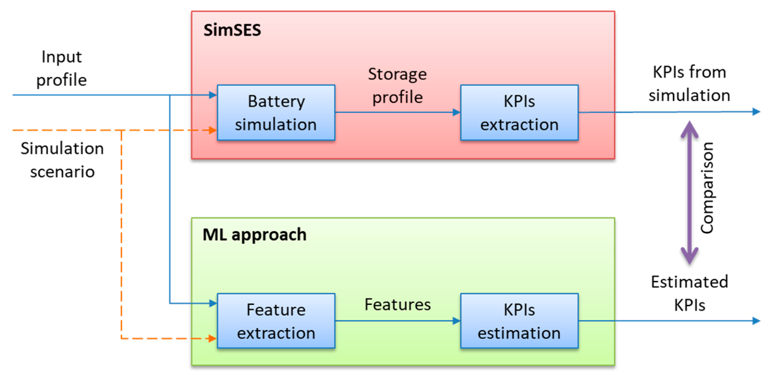
This research explores ML methods to obtain BSS KPIs when they are excited with some input profile (one or several input signals). On one side, an input profile is used as the stimulus of an equivalent circuit model operating in a particular simulation scenario. As a result, the corresponding storage profile is obtained, containing two signals: the storage power supplied to the battery (positive when charging) and the SOC. Then, from the storage profile, several KPIs are extracted summarizing the overall impact of the input profile in the BSS. In this research, the Simulation Tool for Stationary Energy Storage Systems (SimSES) [19] is used for these purposes.
On the other hand, each input profile is characterized using a set of features or attributes: that is, a reduced set of values that approximately describe this input profile. Then, the extracted features are used for an ML model to estimate the corresponding KPIs. This ML model is trained using the datasets described in the following subsection. To evaluate the results produced by the ML approach, the estimated KPIs are compared to the KPIs obtained by SimSES, which are considered as the true values. An overall description of the process is depicted in Figure 2.

2.2. Datasets

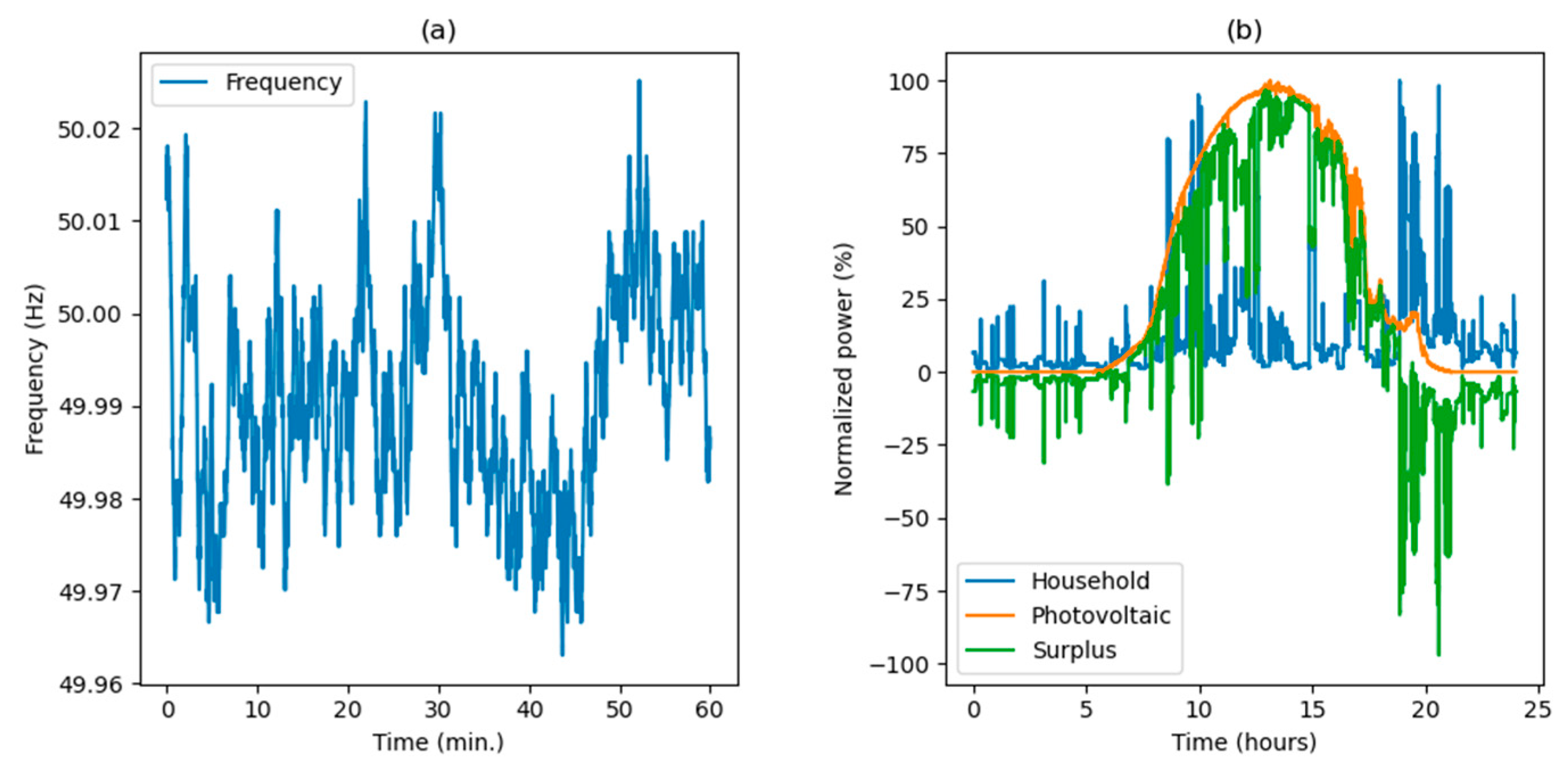
For the FCR application, the evolution of the grid frequency for Continental Europe in a five-year period (2013–2017) is used as the input profile. This information, with a one-second resolution, is provided by the transmission system operator 50 hertz Transmission GmbH [24]. A typical example of the evolution of this signal over one hour is shown in Figure 3a.
For the SCI applications, two signals are required to define an input profile: first, the power demanded over one year for 74 households, information which has been published by the HTW Berlin [25]. Second, SCI requires us to know how much solar power is available. For this purpose, the power generated by a photovoltaic installation at the TU Munich has been recorded during a one-year (2009) experiment [26]. Both signals also have a resolution of one second and, to match their scales, they are normalized in the range of 0–100% of their respective maximum values. Then, the surplus of generation (normalized photovoltaic power minus normalized household demand) is used as a single combined input signal. An example of these two signals for a typical household on a sunny day and the corresponding surplus is shown in Figure 3b.
Until now, the number of instances (examples of input profiles) in the dataset is limited: only one example for FCR and 74 for SCI. These numbers are insufficient to train an ML model. Therefore, to increase the number of instances, each input signal is split into segments of one-day length. In this way, up to 1825 ( 365 × 5 ) FCR and 27,010 ( 365 × 74 ) SCI segments are available. As each FCR segment is analyzed in three different simulation scenarios (two scenarios in the case of SCI), a total of 59,495 instances are available after data preprocessing. Simulation scenarios will be described in the following subsection, while the validity of splitting the input signals into segments of one-day length will be analyzed in the discussion section.
The proper characterization of the input signals is also a key element in the development of these models [27,28,29]. Once a one-day input segment has been obtained, it is described using a feature extraction procedure. For this purpose, no specific application-oriented feature set has been developed. Instead, an off-the-shelf set of general-purpose attributes is used. Up to 16 time-domain and 13 frequency-domain features are computed using several mathematical operations on the input segments. The resulting 29 features are described in [30]. Additionally, the information about the simulation scenario must be included for a fully defined input segment. This can be made by using a single column containing a category value (one out of five possibilities) or, alternatively, using five columns in a one-hot coding scheme. The latter is the solution implemented in this research. Finally, the resulting ML design matrix contains 59,495 rows and 34 columns.

2.3. Simulation Scenarios

To analyze the performance of the ML approach in estimating the KPIs of BSS under different operating conditions, five simulation scenarios have been explored (see Table 1). On one side, two types of battery are considered: a Lithium-Iron-Phosphate (LFP) cathode and a Carbon-Graphite (C) anode; and a Nickel-Manganese-Cobalt-Oxide (NMC) cathode with C anode. The batteries used in FCR applications have a storage capacity of 1.6 MWh and a maximum power of 1.6 MW, while in SCI these parameters are 5 kWh and 5 kW, respectively.
On the other hand, the power electronic required in the BSS is usually modeled as a single unit. However, in certain highly demanding applications such as FCR, an alternative 3-unit modular power electronic system is also considered.
Finally, three different operation strategies have been simulated. In the case of FCR applications, the simulation was executed according to the German regulatory framework [31] where the BSS must provide a certain maximum prequalified power for a predefined time. On the other hand, SCI applications are operated using either greedy or a feed-in damp strategy. In the first case, the solar power surplus is directly devoted to charging the battery. However, to obtain a more stable power fed into the grid, a feed-in damp strategy [26] is also considered.

2.4. Key Performance Indicators

The simulation process yields a storage profile defined by two signals: the storage power (SP) supplied to (or drawn from) the battery; and the SOC. These signals span over the same time interval as the input profile segment, in our case, for one day. Several variables and parameters can be defined from the SP and SOC. They are summarized in Table 2.
Based on the previous definition, three KPIs are defined to characterize the impact of the input profiles on the BSS. The KPIs have been proposed in [23] and are summarized in Table 3. The importance of the KPI “efficiency” has a straightforward interpretation. On the other hand, the other two KPIs have a direct influence on the battery lifetime, as the aging process is due to the number and type of charge-discharge cycles (besides some other factors such as temperature and c-rate) [32], as well as calendric effects [33].
From an ML point of view, the 3 KPIs are the target variables. The ML estimation can be addressed by modeling either a single multiple (3)-target problem or multiple (3) single-target problems. In the first case, the target information is defined in a target matrix containing 59,495 rows and three columns, while in the second case, three target vectors are used, each one containing 59,495 rows. Both approaches have been considered and compared in the following sections.

2.5. Regression Performance Metrics

To compare different options in the modeling process and to select the best algorithms, a regression performance metric must be defined. For that purpose, the coefficient of determination is generally used [34] that, for the k -th KPI, is defined as
R k 2 = 1 i = 1 n y k i y ^ k i 2 i = 1 n y k i y ¯ k 2 ,
where y k i and y ^ k i are the respective actual and estimated values of that KPI for the i -th input profile and y ¯ k is the mean of the actual value of the KPI. The coefficient of determination can be in the range of R k 2 [ , 1 ] . A naïve regressor which always predicts the mean value y ¯ k as the estimation y ^ k i for any input profile would yield a coefficient of determination of R k 2 = 0 . As such, for models with a better prediction than the naïve regressor, the coefficient of determination will be in the range of R k 2 [ 0 ,   1 ] . This result is a very convenient range to compare models and, therefore, R 2 will be the metric used to tune and select the different ML models.
Although R 2 is a very convenient and extended metric, it is mainly algorithm-oriented and does not have an intuitive meaning. Seeking a more human-oriented way to assess the predictions produced by the final selected regressor, a first and more straightforward metric is the error between the actual and the estimated value for a KPI instance. More formally, the prediction error of the k -th KPI corresponding to the i -th input profile can be defined as
e k i = y ^ k i y k i ,
where y k i and y ^ k i are the respective actual and estimated values for that KPI and input profile.
In many cases, the important fact relies on how far the prediction from the actual value is, and not if their difference is positive or negative. For that reason, it is a common practice to measure the absolute values of the differences. Then, the absolute error of the k -th KPI corresponding to the i -th input profile can be defined as
A E k i = e k i = y ^ k i y k i .
The errors for a certain KPI are expressed in the units of that KPI. Then, as these units may be different, it makes no sense to compare the errors for different KPIs. Moreover, even in the case that all the KPIs were in the same unit, they may be in different scales, making a comparison between KPIs meaningless. To tackle this problem, errors can be normalized using a reference value. For instance, a relative absolute error of the k -th KPI corresponding to the i -th input profile can be defined using the actual value as the reference, that is,
r A E k i = e k i y k i = y ^ k i y k i y k i = y ^ k i y k i 1 .
The relative error so defined has the problem that a small absolute error relative to a very low actual value (near 0 ) yields a very large relative error with a significant distortion of the average error. Then, it is usually preferred to make the errors relative, not to a single actual value, but to an average (the mean) of these values. Then, the relative (to the mean) absolute error of the k -th KPI corresponding to the i -th input profile can be defined as
R A E k i = A E k i y ¯ k = e k i y ¯ k = y ^ k i y k i y ¯ k .
For each KPI, the statistical distribution of these errors can be drawn in the form of histograms, probability density functions, or other techniques. In this research, the distribution of the errors will be depicted using boxplots, where the central values are computed using the median as it is more robust than the mean in the presence of outliers (values of errors rarely large). For the same robustness reason, boxplots indicate the statistical dispersion using the 25th and 75th percentile values and the difference between them, called the interquartile range (IQR).
For a dataset containing many input profiles, it is useful to summarize the error values in a single metric, for instance, the average value of the boxplot. For that purpose, the median of the absolute error ( M A E ) and the relative absolute error ( M R A E ) of the k -th KPI are defined as
M A E k = median i A E k i = median i y ^ k i y k i .
M R A E k = median i R A E k i = median i y ^ k i y k i y ¯ k .

2.6. Regression Models

The estimation of the KPIs corresponding to a certain input profile is a good example of an ML regression problem where the target variables (the KPIs) are continuous. Although dozens of regression algorithms have been described in the literature, this paper focuses on three of them: the linear regressor with Tikhonov’s regularization (also known as ridge regressor) [35], the random forest regressor (an ensemble of decision trees) [36], and a feed-forward neural network [37].
Each of the three models contains many parameters and several hyperparameters. To select their values, a hold-out technique has been applied [38]; that is, the dataset (design matrix and target matrix or vector) has been split into three parts, each one containing randomly selected instances: the training (60%), validation (20%), and testing (20%) datasets. First, the training dataset is used to train the models: that is, to select the values of their parameters that minimize an error-related cost function. Second, a validation dataset is used to determine the hyperparameters of the models (including the selection of the best model). Finally, the testing dataset is used to generalize the selected and fitted model: that is, to give an estimation of the error that should be expected when the model is excited with new instances not previously seen.

3. Results

3.1. Optimal Models

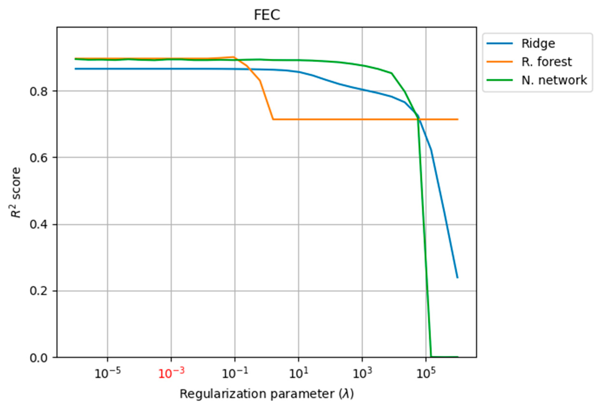
The optimal models are obtained through a validation process which selects the best hyperparameters of the models. An example of this process is shown in Figure 4, where the regression performance (coefficient of determination R 2 ) is drawn for different values of the regularization hyperparameter ( λ ) for a single-target model. In this case, a value of λ = 10 3 has been selected as one that yields the best regression performance.
Using a similar validation process, 100 decision trees have been selected for the random forest regressor. Analogously, an architecture of two hidden layers with 200 nodes each has been the choice for the neural network regressor.
Using these hyperparameters, the R 2 metric has been computed for the predictions obtained using the validation dataset and the six single-target and multiple-target regression algorithms. The results are summarized in Table 4, where the best results for each KPI are in bold font. The random forest regressor overperforms the other two models in all cases. The best results are obtained using a single-target approach for the F E C and n s w a p KPIs, and a multi-target model for the efficiency ( η ). These will be the optimal models used in the remaining sections.

3.2. Generalization of Predictions

Applying the design matrix of the instances in the testing dataset to the optimal regressors, a generalization of the expected errors in the prediction of unseen data can be obtained. In Figure 5, the optimal prediction for each KPI is depicted versus its actual value. As the number of instances in the testing dataset is high (more than ten thousand), a random sample (5%) of these results is plotted to avoid an overcrowded, too-dense, and unreadable graph. The main diagonal (dotted line) in the graph represents a perfect prediction ( y ^ k i = y k i ). As most of the dots are close to this diagonal line, a good result should be expected for the error metrics.
The generalization errors can be summarized using the median absolute error ( M A E ) and the median relative absolute error ( M R A E ) metrics, defined in Section 2.5. The values obtained are described in Table 5, where the selected optimal regressor for each KPI and the corresponding R 2 score are also indicated. The M R A E s are below 8% for all KPIs under investigation.
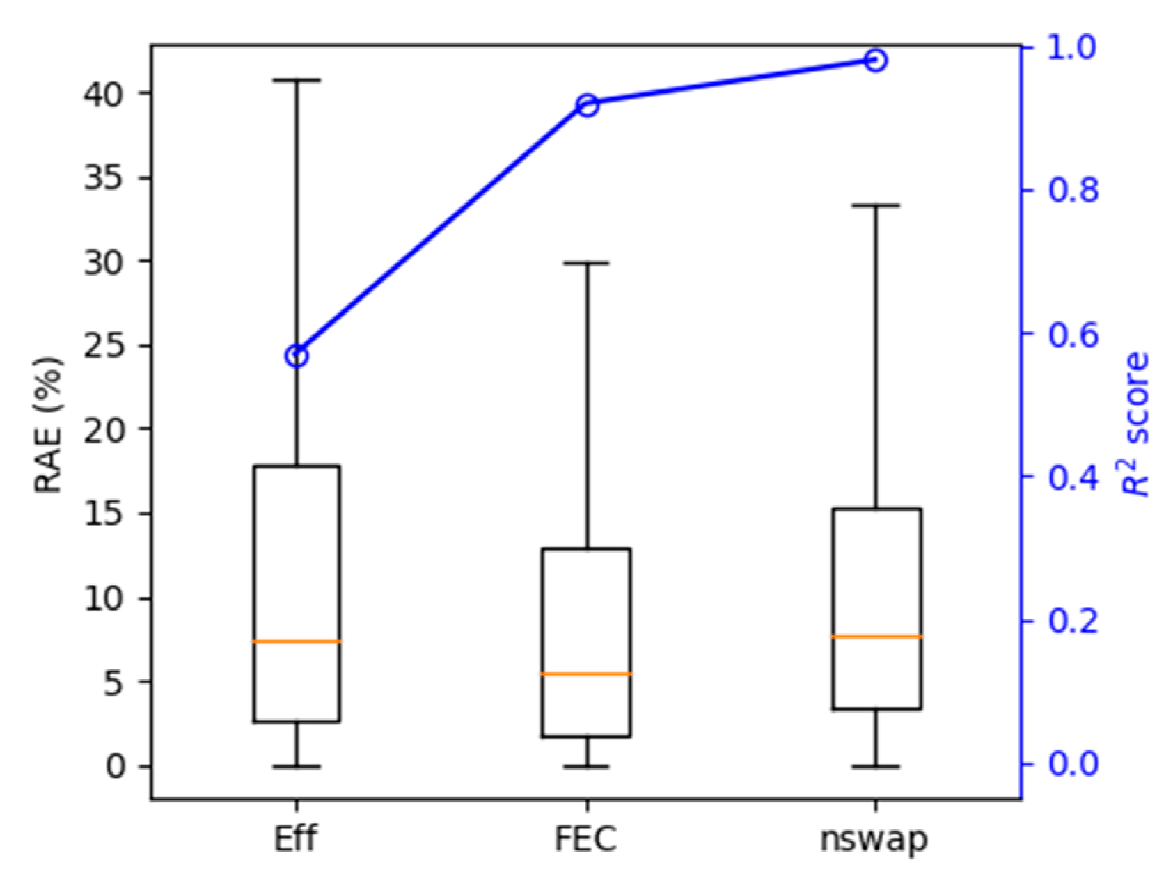
For a more detailed description of the prediction errors, it is important to know not only the average value ( M R A E ) but also the dispersion. For that reason, a boxplot for each KPI is also shown in Figure 6. It can be seen that although the average errors are low, some predictions may have significant errors. However, 75% of the predictions have a R A E below 15%, and 90% are lower than 30%. In this figure, the value of the R 2 score is also plotted.
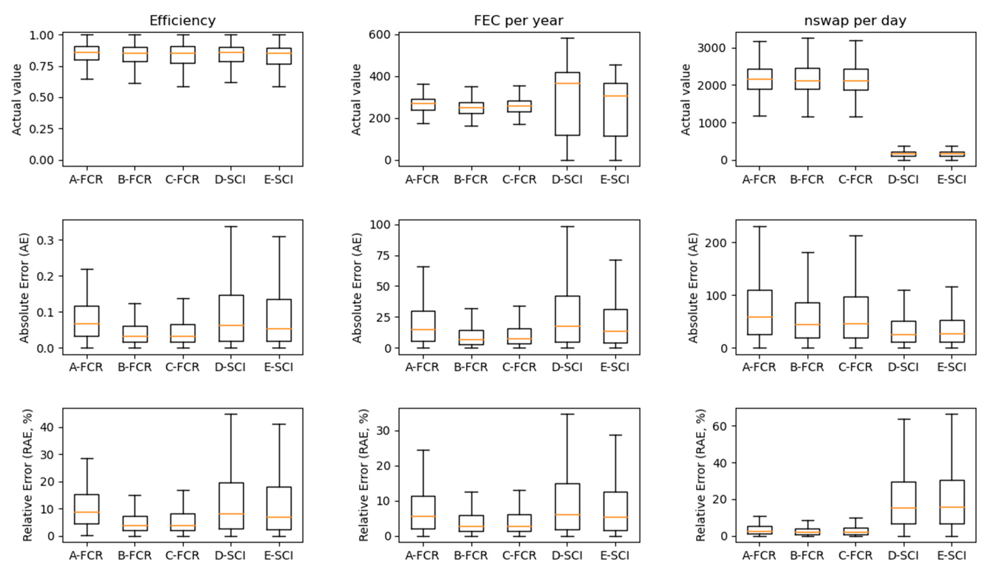
The prediction errors can now be analyzed for each simulation scenario. The corresponding breakdown of the R A E is shown in Figure 7. For a better interpretation of the results, the actual values of the KPIs (first row) and the distribution of the absolute errors (central row) are also depicted in that figure.
The average value ( M R A E ) only slightly depends on the simulation scenario, but this relationship is certainly stronger for error dispersion. The prediction errors of battery efficiency and F E C are more spread out in SCI applications than in FCR, while the opposite happens for the estimations of n s w a p .
A summary of the dependence of the M R A E on the simulation scenario for each KPI is shown in Figure 8. First, for SCI applications, the average prediction error ( M R A E ) is about 10%, slightly higher for the greedy operation than for the feed-in damp. On the other hand, for the FCR applications, the use of one power electronic unit (scenario A-FCR) yields an average error which is three percentual points higher than the errors obtained using three modular units (scenarios B-FCR and C-FCR). It can also be noted that the average errors for n s w a p are significantly higher in the SCI scenarios.
The preceding results show that ML techniques can provide a rough estimation of different KPIs with a medium level of precision. These estimations will probably not be as accurate as those obtained using equation-based simulations or, even more, those based on physical experiments. On the other hand, they can be obtained in much less time. The estimation of the three KPIs presented in Table 3 for a one-year input signal takes, on average, less than 3 s in a desktop computer: that is, approximately 10 7 times less than the physical experiment and 10 3 times less than the SimSES simulation. More than 99% of this time is required for the feature extraction process explained in Section 2.2, which is very dependent on the signal resolution.
The processing times, summarized in Table 6, have been obtained using a computer with a processor based on an Intel® Core™ i7-11700 @ 2.50 GHz processor, with 64 GB of RAM and solid-state disk storage (SSD) of 2TB. The extraction and estimation processes have been developed in Python 3.9 under a Windows 11 operating system, using the scikit-learn 1.0 and TensorFlow 2.10 libraries for the ML-related tasks.

4. Discussion

4.1. Interpreting Results

The results obtained using ML techniques to predict the KPIs of a BSS operating in a certain scenario can be assessed using four approaches as presented in the previous section: a plot comparing predicted and actual values (Figure 5), the M A E error metric, the M R A E error metric, and the R 2 determination coefficient. According to three of these indicators, the best predictions are obtained for n s w a p , closely followed by F E C , and, with a lower performance, E f f . The only exception to that unanimity is found for n s w a p in SCI applications, showing high relative errors (with the best performance in the remaining three criteria). However, this anomaly can be explained because, although the absolute errors in SCI scenarios are low, the actual n s w a p values are very low (see Figure 7), yielding high relative errors.
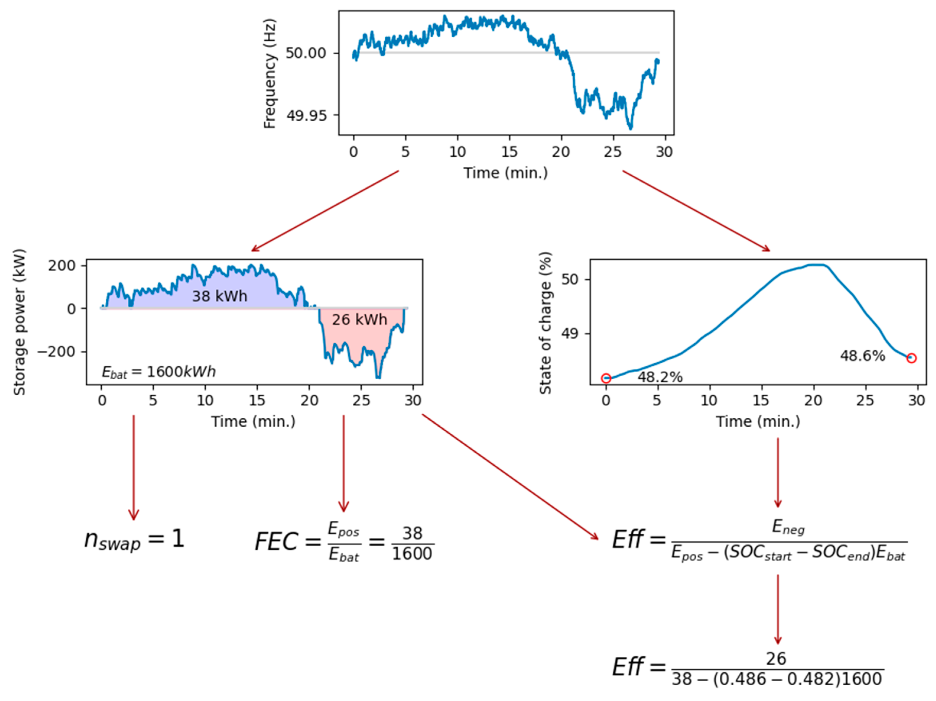
By ordering the KPIs from low to high prediction errors, the following list is obtained: n s w a p , F E C , and E f f . This order can be explained intuitively. Let us consider, for example, a 30 min evolution of the frequency in the electric grid as it is shown in the left part of Figure 9. In an FCR application, the storage power and the SOC of the BSS will follow an evolution as indicated in the central part of the Figure. To predict the number of swaps, it is required to estimate the number of positive power regions (in blue in the graph). On the other hand, to predict the F E C , it is required to estimate not only the number of regions but also their areas. Finally, to predict the efficiency, it is required in addition to estimate the initial and final values of the SOC. So, the more information required to estimate a KPI, the more difficult it should be to predict its value, which explains the results obtained.
On the other hand, when different simulation scenarios are considered, the results show that FCR applications obtain better estimations than SCI. Additionally, for a more detailed analysis, in the FCR case, the KPIs for a BSS with three modular power electronic units obtain (slightly) better estimations than those simulations where a single power electronic unit is used. Finally, the estimation of KPIs in the feed-in damp SCI scenario is better than the estimations for the greedy SCI strategy.
To gain some intuition on the reasons for these results, the smoothness of the input profiles will be considered. The underlying idea is that the estimation of the KPIs must be easier for a smooth input profile than for those with sudden unpredictable changes. To depict these ideas, two random examples are drawn in Figure 10.
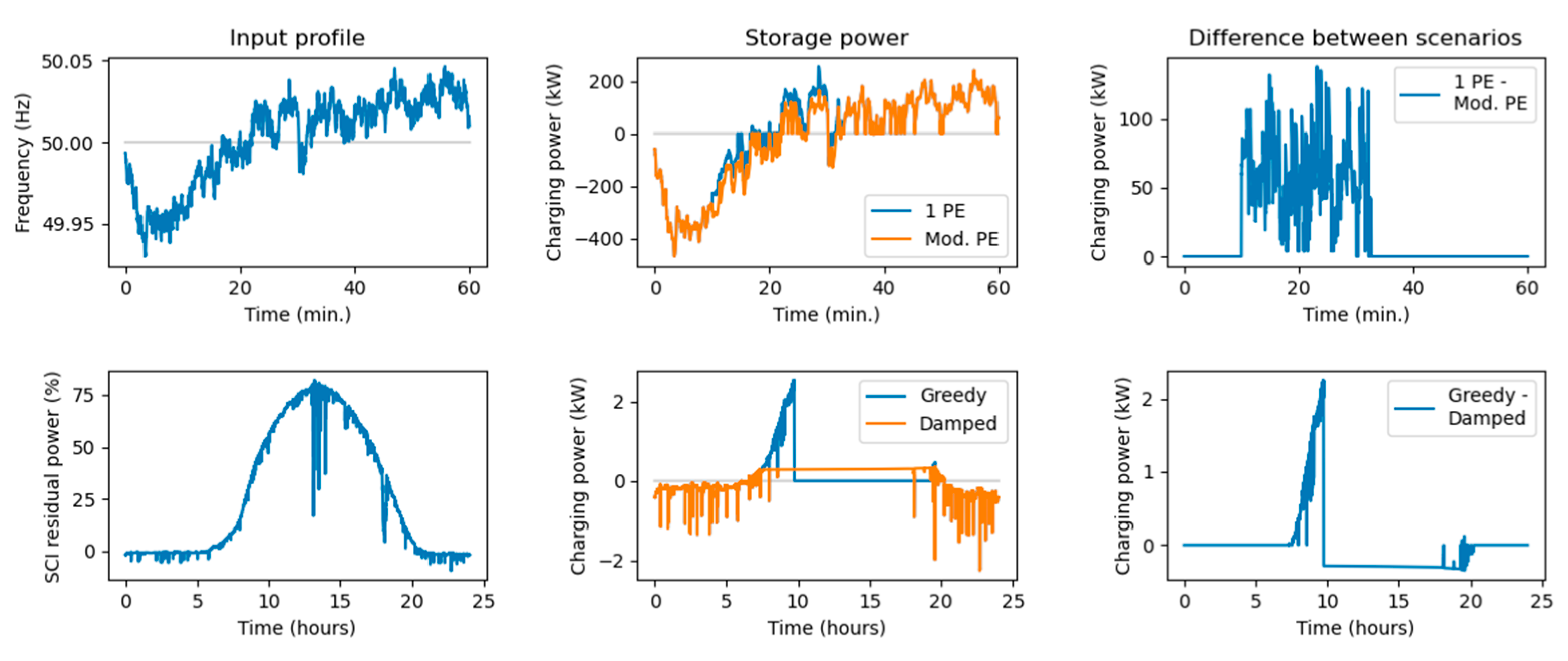
In the top part, a 60 min FCR simulation is shown, while in the bottom row, a one-day SCI application is considered. In the first column, the input profiles are plotted, clearly showing that significantly more unpredicted events occur in the SCI case. In this example (a household), the sudden changes in SCI are probably due to an increase in the power demand during lunchtime and after-work activities. On the other hand, for the FCR application, the frequency signal responds to an aggregated demand showing a more stable evolution.
To explain the differences between the prediction performances in different operation strategies, the storage power in the BSS is considered, as is shown in the upper (FCR) and lower (SCI) rows of the central column in Figure 10. For an easy reading of the signals in the example, the differences between the charging power in both scenarios are plotted in the right column of the Figure.
It can be seen that the smoothness of the signal in different operation strategies is not so different than those seen when comparing different applications (FCR vs. SCI). However, in the FCR 1PE scenario, the charging power is always equal to or greater than the modular PE operation. As only one power electronic unit is available, a less flexible operation can be provided, yielding (slightly) less smooth signals. A similar situation occurs in SCI applications where the charging power signal in the greedy operation directly follows the unpredicted changes in the photovoltaic residual power (photovoltaic generation minus household demand), while the feed-in damp operation attenuates this impact by a more tempered charge of the battery, also yielding (slightly) smoother signals. These reasons explain the differences found in prediction performances between applications and operation strategies.

4.2. Learning Curves

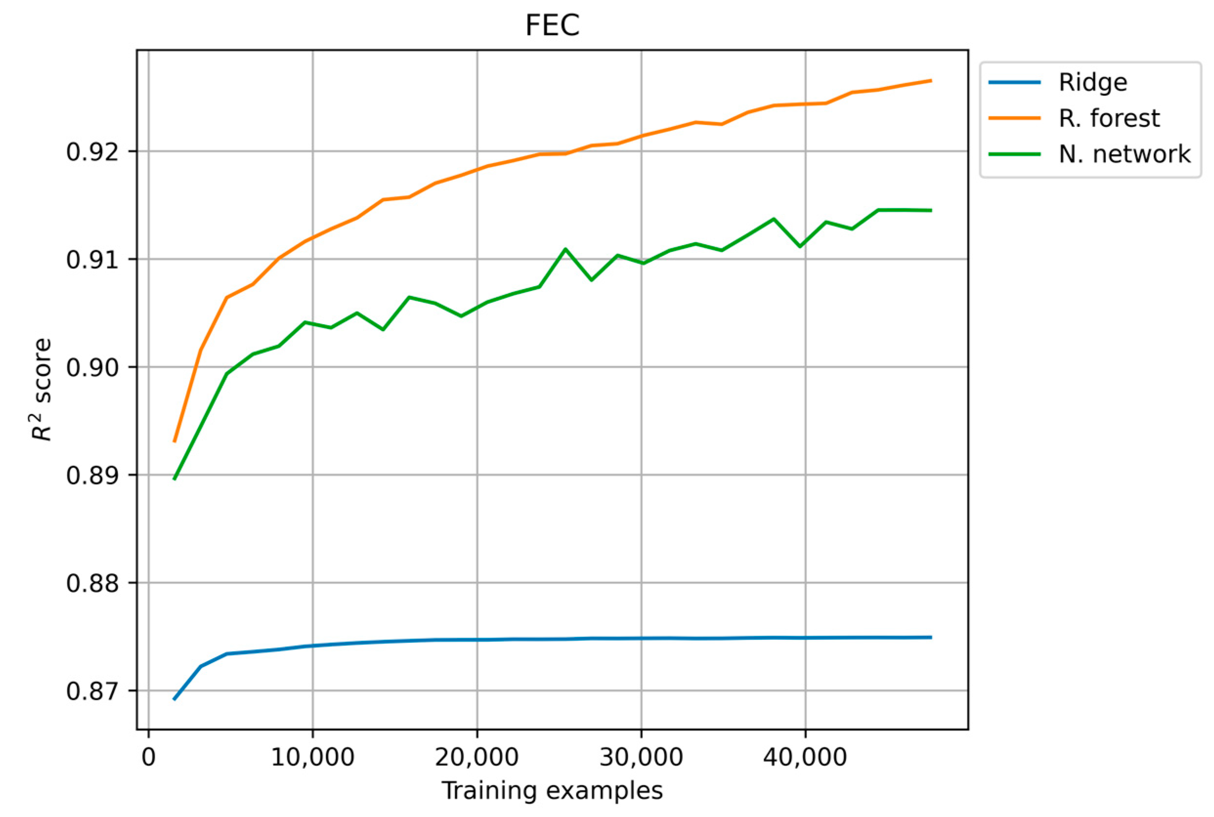
Once the hyperparameters have been selected in the validation process, the training and validation datasets are unified in an extended training dataset containing 80% of the total number of instances: that is, about 50,000 instances. To assess if this is a sufficient amount of training samples, a learning curve is plotted, where the regression performance ( R 2 metric) is computed for an increasing number of training examples. The resulting learning curves for a particular KPI ( F E C ) and three single-target regressors are depicted in Figure 11. Similar results are obtained for other KPIs and regressors. It can be seen that the ridge regressor reaches the maximum performance for about 10,000 training instances. Still, neither the random forest nor the neural network regressors achieve a maximum flat performance for the available number of training samples.
These results can be explained by considering the number of parameters required to define each model, which are summarized in Table 7. The higher the number of parameters, the more complex a model is, and a greater number of instances is required for its training. So, if larger datasets were available, better estimations should be expected.

4.3. Length of Input Profiles

The design matrix used to train the models was generated by splitting each one-year-length input into segments of one-day length. By decreasing the length of these segments, a greater number of segments was obtained. To check the dependence of the values of a certain KPI on the length of segments, a one-year-length input signal is split into several segments. For each segment, several values of that KPI are obtained: the shorter the segment, the greater the number of values. These values can be statistically described using, for instance, their median and IQR. The relationship between these statistics and the length of the segments is depicted for an FCR scenario in Figure 12 and for an SCI application in Figure 13. Similar results are obtained for the remaining scenarios.
In these Figures, it can be seen that the statistical distribution of the values of the KPIs remains stable if the input profiles are split up into one-day-length segments. For shorter segments, a qualitative change in the KPI values should be expected. So, it is not advisable to increase the datasets by reducing the length of segments.

4.4. Sampling Times

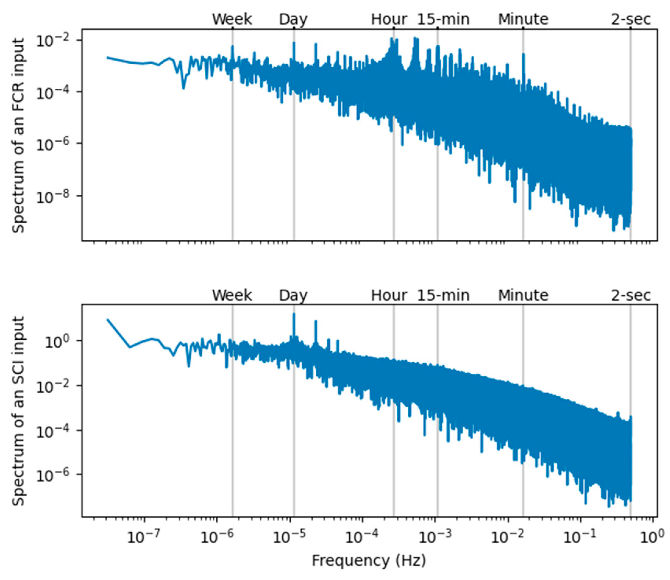
Input profiles are available in the datasets with a resolution of one second and a length of one year. That means that each input profile contains 31,536,000 values. Therefore, processing these high-resolution signals is computationally demanding. To explore if it is possible to down-sample these profiles, a frequency analysis has been performed. For that purpose, the spectrum of amplitude is obtained for each input profile, using a fast Fourier transform (FFT) algorithm.
The results for an example of FCR and SCI input profiles are shown in Figure 14. It can be seen that the highest frequency of a significant harmonic for an FCR signal corresponds to a sampling period of about one minute. For the SCI input profiles, this harmonic corresponds to about four hours. Therefore, input profiles could be significantly down-sampled, using resolutions higher than 30 s for FCR and two hours for SCI.

5. Conclusions

This research has shown that the behavior of a BSS can successfully be estimated from its input power signal using machine learning (ML) techniques, which can be applied to unseen new datasets as long as they have the same statistical distribution: that is, the input profiles are independent and identically distributed (IID). Different KPIs summarizing the functioning of the battery have been predicted with an average relative error ( M R A E ) of less than 10%. These average errors may differ depending on the KPI and the battery operation scenario, ranging from 2% in the better case to 16% in the worst case.
Although the precisions estimating the battery KPIs are not very high, the ML approach proposed in this article offers the advantage of obtaining a prediction in a relatively short time (a few seconds), a remarkable result compared to the computing effort required when using simulations based on electric-equivalent circuits (several hours).
The precision obtained in this research highly depends on the number of training examples available. As the learning curves have shown, the selected ML algorithm (a random forest regressor) has not reached its maximum performance and better predictions should be expected with a larger training dataset.
The predicting models are valid for the same conditions employed to obtain the datasets. If the application, the operation strategy, and/or the parameters of the battery system change, a new ML model has to be trained from the corresponding dataset.
From the previous paragraphs, it can be stated that the methods proposed in this research have two main limitations: they can only be used in cases where similar examples have been previously analyzed, either in lab tests or by equation-based simulations; and, on the other hand, the estimation of KPIs through ML techniques does include an estimation error (10% on average in our study).
ML techniques are a very powerful tool to have at hand, but they do not replace an in-depth analysis and domain knowledge-based discussion of results altogether. As applied herein, they do not eliminate the need for precise physical-model-based simulations or lab-controlled experimentation, but they can offer a first and very fast rough approximation of the expected behavior of a BSS.
The results presented in this article, mainly those concerning to F E C and n s w a p , indicate that ML techniques can probably be extended to estimate the SOH of a battery after a given input profile, a question that the authors will research in the future.

Author Contributions

Conceptualization, H.H.; methodology, J.L.; software, J.L. and B.T.; validation, H.H., D.L. and C.L.; resources, H.H. and C.L.; writing—original draft preparation, J.L. and D.L.; writing—review and editing, B.T., H.H. and C.L. All authors have read and agreed to the published version of the manuscript.

Funding

This research received no external funding.

Data Availability Statement

Publicly available datasets were analyzed in this study. This data can be found here: https://www.50hertz.com/de/Transparenz/Kennzahlen/Regelenergie/ArchivNetzfrequenz (accessed on 19 July 2023); https://solar.htw-berlin.de/elektrische-lastprofile-fuer-wohngebaeude/ (accessed on 19 July 2023).

Acknowledgments

The authors thank Andreas Jossen and Julius Bahrke for their insightful and encouraging comments during this research.

Conflicts of Interest

The authors declare no conflict of interest.

References

  1. Zhao, Y.; Pohl, O.; Bhatt, A.I.; Collis, G.E.; Mahon, P.J.; Rüther, T.; Hollenkamp, A.F. A Review on Battery Market Trends, Second-Life Reuse, and Recycling. Sustain. Chem. 2021, 2, 167–205. [Google Scholar] [CrossRef]
  2. Figgener, J.; Stenzel, P.; Kairies, K.-P.; Linßen, J.; Haberschusz, D.; Wessels, O.; Angenendt, G.; Robinius, M.; Stolten, D.; Sauer, D.U. The Development of Stationary Battery Storage Systems in Germany–A Market Review. J. Energy Storage 2020, 29, 101153. [Google Scholar] [CrossRef]
  3. Figgener, J.; Hecht, C.; Haberschusz, D.; Bors, J.; Spreuer, K.G.; Kairies, K.-P.; Stenzel, P.; Sauer, D.U. The Development of Battery Storage Systems in Germany: A Market Review (Status 2023). arXiv 2023, arXiv:2203.06762v3. [Google Scholar] [CrossRef]
  4. Han, B.; Bompard, E.; Profumo, F.; Xia, Q. Paths toward Smart Energy: A Framework for Comparison of the EU and China Energy Policy. IEEE Trans. Sustain. Energy 2014, 5, 423–433. [Google Scholar] [CrossRef]
  5. Luís Schaefer, J.; Siluk, J.C.M.; Siluk, M.; De Carvalho, P.S. Critical Success Factors for the Implementation and Management of Energy Cloud Environments. Int. J. Energy Res. 2022, 46, 13752–13768. [Google Scholar] [CrossRef]
  6. Alhasnawi, B.N.; Jasim, B.H.; Esteban, M.D.; Guerrero, J.M. A Novel Smart Energy Management as a Service over a Cloud Computing Platform for Nanogrid Appliances. Sustainability 2020, 12, 9686. [Google Scholar] [CrossRef]
  7. ENTSO-E. Commission Regulation (EU) 2017/1485 of 2 August 2017 Establishing a Guideline on Electricity Transmission System Operation; ENTSO-E: Brussels, Belgium, 2017. [Google Scholar]
  8. Hesse, H.C.; Schimpe, M.; Kucevic, D.; Jossen, A. Lithium-Ion Battery Storage for the Grid—A Review of Stationary Battery Storage System Design Tailored for Applications in Modern Power Grids. Energies 2017, 10, 2107. [Google Scholar] [CrossRef] [Green Version]
  9. Resch, M.; Buehler, J.; Klausen, M.; Sumper, A. Impact of Operation Strategies of Large Scale Battery Systems on Distribution Grid Planning in Germany. Renew. Sustain. Energy Rev. 2017, 74, 1042–1063. [Google Scholar] [CrossRef] [Green Version]
  10. Henni, S.; Becker, J.; Staudt, P.; vom Scheidt, F.; Weinhardt, C. Industrial Peak Shaving with Battery Storage Using a Probabilistic Forecasting Approach: Economic Evaluation of Risk Attitude. Appl. Energy 2022, 327, 120088. [Google Scholar] [CrossRef]
  11. Gong, H.; Ionel, D.M. Improving the Power Outage Resilience of Buildings with Solar Pv through the Use of Battery Systems and Ev Energy Storage. Energies 2021, 14, 5749. [Google Scholar] [CrossRef]
  12. Lund, P.D. Improving the Economics of Battery Storage. Joule 2020, 4, 2543–2545. [Google Scholar] [CrossRef]
  13. Eyer, J.; Corey, G. Energy Storage for the Electricity Grid: Benefits and Market Potential Assessment Guide. Sandia Natl. Lab. 2010, 20, 5. [Google Scholar]
  14. Schmidt, A.P.; Bitzer, M.; Imre, Á.W.; Guzzella, L. Experiment-Driven Electrochemical Modeling and Systematic Parameterization for a Lithium-Ion Battery Cell. J. Power Sources 2010, 195, 5071–5080. [Google Scholar] [CrossRef]
  15. Liu, K.; Gao, Y.; Zhu, C.; Li, K.; Fei, M.; Peng, C.; Zhang, X.; Han, Q.-L. Electrochemical Modeling and Parameterization towards Control-Oriented Management of Lithium-Ion Batteries. Control Eng. Pract. 2022, 124, 105176. [Google Scholar] [CrossRef]
  16. Miranda, D.; Gonçalves, R.; Wuttke, S.; Costa, C.M.; Lanceros-Méndez, S. Overview on Theoretical Simulations of Lithium-Ion Batteries and Their Application to Battery Separators. Adv. Energy Mater. 2023, 13, 2203874. [Google Scholar] [CrossRef]
  17. Xia, L.; Najafi, E.; Li, Z.; Bergveld, H.J.; Donkers, M.C.F. A Computationally Efficient Implementation of a Full and Reduced-Order Electrochemistry-Based Model for Li-Ion Batteries. Appl. Energy 2017, 208, 1285–1296. [Google Scholar] [CrossRef]
  18. Moškon, J.; Gaberšček, M. Transmission Line Models for Evaluation of Impedance Response of Insertion Battery Electrodes and Cells. J. Power Sources Adv. 2021, 7, 100047. [Google Scholar] [CrossRef]
  19. Möller, M.; Kucevic, D.; Collath, N.; Parlikar, A.; Dotzauer, P.; Tepe, B.; Englberger, S.; Jossen, A.; Hesse, H. SimSES: A Holistic Simulation Framework for Modeling and Analyzing Stationary Energy Storage Systems. J. Energy Storage 2022, 49, 103743. [Google Scholar] [CrossRef]
  20. Gasper, P.; Collath, N.; Hesse, H.C.; Jossen, A.; Smith, K. Machine-Learning Assisted Identification of Accurate Battery Lifetime Models with Uncertainty. J. Electrochem. Soc. 2022, 169, 80518. [Google Scholar] [CrossRef]
  21. Aykol, M.; Herring, P.; Anapolsky, A. Machine Learning for Continuous Innovation in Battery Technologies. Nat. Rev. Mater. 2020, 5, 725–727. [Google Scholar] [CrossRef]
  22. Wei, Z.; He, Q.; Zhao, Y. Machine Learning for Battery Research. J. Power Sources 2022, 549, 232125. [Google Scholar] [CrossRef]
  23. Kucevic, D.; Tepe, B.; Englberger, S.; Parlikar, A.; Mühlbauer, M.; Bohlen, O.; Jossen, A.; Hesse, H. Standard Battery Energy Storage System Profiles: Analysis of Various Applications for Stationary Energy Storage Systems Using a Holistic Simulation Framework. J. Energy Storage 2020, 28, 101077. [Google Scholar] [CrossRef]
  24. 50Hertz Transmission GmbH. Archiv Netzfrequenz (in German): Daten Der Entso-E; 50Hertz Transmission GmbH: Berlin, Germany, 2019; Available online: https://www.50hertz.com/de/Transparenz/Kennzahlen/Regelenergie/ArchivNetzfrequenz (accessed on 19 July 2023).
  25. Tjaden, T.; Bergner, J.; Weniger, J.; Quaschning, V.; Solarspeichersysteme, F. Repräsentative Elektrische Lastprofile Für Wohngebäude in Deutschland Auf 1-Sekündiger Datenbasis. Hochsch. Für Tech. Und Wirtsch. HTW Berl. 2015. Available online: https://solar.htw-berlin.de/elektrische-lastprofile-fuer-wohngebaeude/ (accessed on 19 July 2023).
  26. Truong, C.N.; Naumann, M.; Karl, R.C.; Müller, M.; Jossen, A.; Hesse, H.C. Economics of Residential Photovoltaic Battery Systems in Germany: The Case of Tesla’s Powerwall. Batteries 2016, 2, 14. [Google Scholar] [CrossRef] [Green Version]
  27. Luque, J.; Personal, E.; Perez, F.; Romero-Ternero, M.; Leon, C. Low-Dimensional Representation of Monthly Electricity Demand Profiles. Eng. Appl. Artif. Intell. 2023, 119, 105728. [Google Scholar] [CrossRef]
  28. Luque, J.; Carrasco, A.; Personal, E.; Pérez, F.; León, C. Customer Identification for Electricity Retailers Based on Monthly Demand Profiles by Activity Sectors and Locations. IEEE Trans. Power Syst. 2023. [Google Scholar] [CrossRef]
  29. Luque, J.; Personal, E.; Garcia-Delgado, A.; Leon, C. Monthly Electricity Demand Patterns and Their Relationship with the Economic Sector and Geographic Location. IEEE Access 2021, 9, 86254–86267. [Google Scholar] [CrossRef]
  30. Yan, X.; Jia, M. A Novel Optimized SVM Classification Algorithm with Multi-Domain Feature and Its Application to Fault Diagnosis of Rolling Bearing. Neurocomputing 2018, 313, 47–64. [Google Scholar] [CrossRef]
  31. 50Hertz Transmission GmbH. Prequalification Process for Balancing Service Providers (FCR, aFRR, mFRR) in Germany . June 2022. Available online: https://www.regelleistung.net/xspproxy/api/StaticFiles/Regelleistung/Infos_f%C3%BCr_Anbieter/Wie_werde_ich_Regelenergieanbieter_Pr%C3%A4qualifikation/Pr%C3%A4qualifikationsbedingungen_FCR_aFRR_mFRR/PQ-Bedingungen-03.06.2022(englisch).pdf (accessed on 19 July 2023).
  32. Naumann, M.; Spingler, F.B.; Jossen, A. Analysis and Modeling of Cycle Aging of a Commercial LiFePO4/Graphite Cell. J. Power Sources 2020, 451, 227666. [Google Scholar] [CrossRef]
  33. Naumann, M.; Schimpe, M.; Keil, P.; Hesse, H.C.; Jossen, A. Analysis and Modeling of Calendar Aging of a Commercial LiFePO4/Graphite Cell. J. Energy Storage 2018, 17, 153–169. [Google Scholar] [CrossRef]
  34. Di Bucchianico, A. Coefficient of Determination (R2). Encycl. Stat. Qual. Reliab. 2008. [Google Scholar] [CrossRef]
  35. McDonald, G.C. Ridge Regression. Wiley Interdiscip. Rev. Comput. Stat. 2009, 1, 93–100. [Google Scholar] [CrossRef]
  36. Segal, M.R. Machine Learning Benchmarks and Random Forest Regression; UCSF: San Francisco, CA, USA, 2004; Available online: https://escholarship.org/uc/item/35x3v9t4 (accessed on 19 July 2023).
  37. Specht, D.F. A General Regression Neural Network. IEEE Trans. Neural Netw. 1991, 2, 568–576. [Google Scholar] [CrossRef] [PubMed] [Green Version]
  38. Arlot, S.; Celisse, A. A Survey of Cross-Validation Procedures for Model Selection. Stat. Surv. 2010, 4, 40–79. [Google Scholar] [CrossRef]
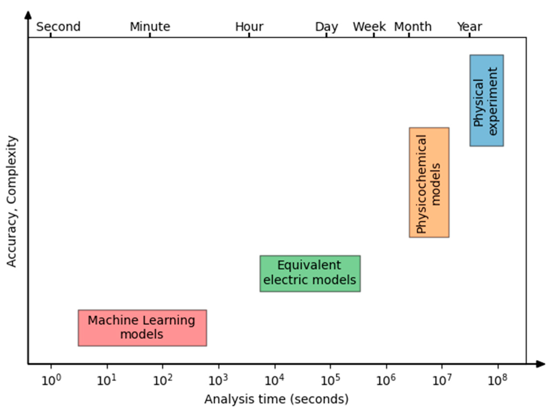
Figure 1. Comparison of different analysis methods of battery cell and system behavior.
Energies 16 05548 g001
Figure 2. General description of the research methodology. “SimSES” refers to a battery time series simulation tool incorporating an ECM battery model [16].
Energies 16 05548 g002
Figure 3. Example of input profiles: (a) Evolution of the frequency in Continental Europe for one hour; (b) Normalized values of the photovoltaic power generated in a typical sunny day, the electric power demanded by a household, and the difference between them (surplus).
Energies 16 05548 g003
Figure 4. Selection of the regularization parameter. The value λ = 10 3 is selected for the three regression models.
Energies 16 05548 g004
Figure 5. Generalization results: estimated values of the KPIs using the optimal predictor versus their actual value. Results obtained for a random 5% of the testing dataset.
Energies 16 05548 g005
Figure 6. Relative absolute errors ( R A E ) and R 2 score of the optimal prediction for each KPI using the testing dataset.
Energies 16 05548 g006
Figure 7. Errors of the optimal prediction for each KPI and each simulation scenario. Top row: actual value; central row: absolute errors ( A E ); bottom row: relative absolute errors ( R A E ). Results obtained using the testing dataset.
Energies 16 05548 g007
Figure 8. Mean relative absolute errors ( M R A E ) of the optimal prediction for each KPI and each simulation scenario. Results obtained using the testing dataset.
Energies 16 05548 g008
Figure 9. Example of obtaining KPIs for an FCR application. Left: evolution of the frequency in the electric grid; center: storage power (top) and state-of-charge (bottom) of the battery system; right: derivation of the KPIs.
Energies 16 05548 g009
Figure 10. Examples of random FCR and SCI segments. Left: input profiles; center: storage power with two different operation strategies; right: difference in charging power between the two strategies.
Energies 16 05548 g010
Figure 11. Learning curves for regression models predicting F E C .
Energies 16 05548 g011
Figure 12. Relationship between the values of the KPIs and the length of the segments in an FCR scenario. The median and IQR of the KPI are plotted.
Energies 16 05548 g012
Figure 13. Relationship between the values of the KPIs and the length of the segments in an SCI scenario. The median and IQR of the KPI are plotted.
Energies 16 05548 g013
Figure 14. Frequency analysis of an FCR (top) and an SCI (bottom) input profile.
Energies 16 05548 g014
Table 1. Simulation scenarios.
ScenarioA-FCRB-FCRC-FCRD-SCIE-SCI
ApplicationFCRFCRFCRSCISCI
Battery typeLFP:CLFP:CNMC:CLFP:CLFP:C
Storage Capacity1.6 MWh1.6 MWh1.6 MWh5 kWh5 kWh
Maximum Power1.6 MW1.6 MW1.6 MW5 kW5 kW
Power ElectronicSingle unit3 modular3 modularSingle unitSingle unit
Operation strategyFCR regulations Germany (status 2021)GreedyFeed-in damp
Table 2. Variables and parameters describing the storage profile signals.
NameDescription
E b a t Energy storage capacity of the battery
E p o s Positive energy (supplied to the battery); when S P > 0
E n e g Negative energy (drawn from the battery); when S P < 0
S O C s t a r t SOC at the start of the signal
S O C e n d SOC at the end of the signal
Table 3. Key Performance Indicators (KPIs).
NameDescriptionExpression
η Efficiency E n e g E p o s S O C s t a r t S O C e n d E b a t
F E C Full Equivalent Cycles E p o s E b a t
n s w a p Number of swaps
(charging-discharging)
Defined in [23]
Table 4. Performance of different regression models ( R 2 score). Optimal models in boldface and green background.
KPISingle TargetMulti-Target
RidgeR. ForestN. NetworkRidgeR. ForestN. Network
η0.0110.122−0.0640.0160.570−0.034
FEC0.8110.9270.9180.8660.9190.902
ηswap0.9540.9850.9650.9530.9800.962
Table 5. Generalization errors of the optimal models ( M R A E metric and R2 score).
KPIMAEMARER2 ScoreOptimal Regressor
AlgorithmTargets
η0.0567.38%0.570R. forestMulti-target
FEC14.425.42%0.919R. forestSingle target
ηswap28.047.72%0.980R. forestSingle target
Table 6. Average computing times required to estimate the 3 KPIs from a one-year-length input profile.
AlgorithmProcessing Time
AbsoluteRelative
Feature extraction2391 ms.99.41%
KPI estimation14 ms.0.59%
Total2406 ms.100.00%
Table 7. Number of parameters of the regression models.
KPIRegression Algorithm
R i d g e R. ForestN. Network
η 35 21,138,550 47,401
F E C 35 21,236,200 47,401
n s w a p 35 18,130,410 47,401
Multi-target 105 29,910,412 47,803
Disclaimer/Publisher’s Note: The statements, opinions and data contained in all publications are solely those of the individual author(s) and contributor(s) and not of MDPI and/or the editor(s). MDPI and/or the editor(s) disclaim responsibility for any injury to people or property resulting from any ideas, methods, instructions or products referred to in the content.