Abstract
The integration of PV and energy storage systems (ESS) into buildings is a recent trend. By optimizing the component sizes and operation modes of PV-ESS systems, the system can better mitigate the intermittent nature of PV output. Although various methods have been proposed to optimize component size and achieve online energy management in PV-ESS systems, the optimal interconnection between them has received less attention. In order to maximize the effectiveness of systems with limited component sizes and address the impact of uncertainty on the system, an optimization framework is proposed for determining the optimal size of the PV-ESS system. The proposed framework consists of five parts: determination of optimal size, analysis of component output characteristics, system state prediction, parameter calibration of energy management strategies, and update of system components output features, and it considers uncertain factors, including climate, different components, and battery degradation caused by irregular charging and discharging, to establish the model for energy saving. To validate the results, four different climates in a year were considered. The obtained results indicate that the proposed framework can effectively achieve the optimal working state of the system, realizing a matching degree of 94.55% between the offline size optimization and online management strategy. The proposed framework’s universality and effectiveness were demonstrated through simulation analysis across four cities with different climates in China.
1. Introduction
In recent years, power systems worldwide have gradually advanced towards “decentralization”, “decarbonization”, and “democratization” to control power costs, alleviate the aging of infrastructure, improve the resilience and reliability of power systems, reduce carbon dioxide emissions and mitigate climate change, and provide reliable power for areas lacking power infrastructure [1,2]. For the effective deployment of distributed energy, PV-ESS systems have become a reliable alternative and have been employed extensively in recent years [3,4]. Although developments in the global energy industry have stagnated to a certain extent since 2018, the new energy market forecast released by the International Energy Agency (IEA) in 2019 states that the installation of PV systems in commercial buildings, residential buildings, and other areas will change the traditional mode of power generation and consumption, and that these measures will gradually lead to the “secondary Renaissance” of the new energy market [5,6]. Therefore, many researchers have carried out a series of studies on this topic [7,8,9].
Through the deployment of home energy management systems (HEMS) and the implementation of demand side management (DSM) in residential buildings, peak shaving, valley filling, and load regulation can be achieved, thereby improving the power quality and maintaining power system stability. PV-ESS systems can be more beneficial to residential users, thereby achieving high clean energy penetration and sustainable development [10]. The progress in lithium-ion battery-related technologies in recent years has increased its energy density and reduced its cost. Coupled with the vigorous developments in the energy industry, the combination of distributed energy storage and new energy technology has become an alternate technical route. Due to the gradual diversification of energy storage devices, optimizing the component sizes of the system according to the radiation and load in the region can maximize the benefits of high energy utilization [11,12]. Recently, Al-Ghussain et al. discussed the different types of ESS that can be applied to PV and wind energy systems. Furthermore, a university campus was selected for a case study, by which the significant impact of the type and size of ESS on the economics of the system was proved [13]. Wang et al. studied DSM in commercial buildings integrated with PV systems, ESS, and grid-connected electric vehicles and demonstrated that a modest number of electric vehicles (EV) can reduce overall operating costs, revealing the benefits of large-scale EV integration into smart buildings in the future [14]. Abbassi et al. accurately modeled a PV system with a hybrid energy storage system (HESS). By controlling the power outputs of each energy storage unit, it was shown that the configuration of the super-capacitor (SC) could avoid the rapid charge and discharge cycles and thus alleviate the degradation of the battery [15]. The above studies have all proved that, in addition to the technical and environmental advantages, the collaboration of PV-ESS systems can effectively improve the system’s economics and reduce charging costs.
1.1. Literature Review
At present, there are a number of studies on the size optimization of distributed power generation devices in residential applications. Sandhu et al. proposed a method for optimizing the size of BESS to reduce output power fluctuations generated by wind and solar power. Further, the particle swarm optimization (PSO) algorithm was used to determine the optimal sizing of ESS [16]. Babacan et al. considered the cost of ESS, land, and installation and developed a two-layer optimization method based on a genetic algorithm (GA) to reduce the voltage fluctuations caused by the instability of PV generation by installing BESS between the power distribution system nodes [17]. Chaudhari et al. proposed a method to determine the optimal size of the BESS. By establishing an artificial neural network (ANN), the optimal size of BESS was evaluated according to the ability of the system to regulate frequency and voltage [18]. Wang et al. proposed a method to obtain the optimal size of a multi-source power system according to its different working modes. Considering the system reliability, an energy management strategy using the discrete Fourier transform was proposed [19,20]. To achieve the minimum purchase and operation costs in the system, Alhaider et al. optimized the number of PV panels and the size of the ESS based on the randomness of PV output and converted the problem into a mixed integer linear programming problem. The decomposition strategy was then used to solve the optimization problem [21,22,23]. Eltamally et al. considered various components, including wind, PV, batteries, and diesel generators, and designed fuzzy logic controllers to achieve demand response. Additionally, two improved search algorithms were successively proposed to optimize the size of each component [24,25]. Khorramdel et al. conducted a cost–benefit analysis on the microgrid and considered 12 possible scenarios in ESS during operation. On this basis, particle swarm optimization was used for the size optimization of the ESS to minimize the cost [26]. In the above research, the output of the PV-ESS system was optimized using algorithms such as the genetic algorithm and particle swarm algorithm. The optimal system size was then obtained through comparison. However, most scheduling models are multi-constrained, nonlinear, and non-real-time. Due to the system characteristics, during the actual operation, the HEMS cannot perform DSM on the load according to the output curves obtained using these types of optimization algorithms.
Meanwhile, research on methods to achieve efficient load dispatching and increased renewable energy consumption through demand response for reducing household power consumption has attracted considerable attention. Aryani et al. proposed a control strategy based on model predictive control (MPC) to smoothen the output fluctuations in PV systems through battery ESS. The battery charging and discharging action were observed while considering some constraints, such as battery power and battery SOC, to effectively track the parameter value of system output [27]. Ye et al. proposed an adaptive hybrid optimization algorithm for ESS management, which uses a rule-based method for energy storage management in PV system-integrated electric vehicle charging stations [28]. Olaszi et al. analyzed three scheduling strategies for PV-ESS systems: rule-based strategy, adaptive algorithm-based strategy, and energy market-oriented remote-control strategy [29]. Korjani et al. identified and clustered the characteristics of consumer groups based on online energy management tools and determined the working status of PV-ESS according to the established rules [30]. Wang also used MPC to analyze the power scheduling problem in the PV-ESS microgrid to ensure that the power scheduling in the system is flexible and robust [31]. However, there is little consideration of the current scheduling problem of the PV-ESS system in these studies. Due to the intermittence and instability of PV output, accurate prediction through analysis of historical data is critical to the planning and management of the system [32,33]. At present, the traditional methods for forecasting the source end generation capacity of renewable energy sources include physical and statistical methods. With the development of soft computing technology, the prediction model based on artificial intelligence is often considered superior to physical and statistical methods because of its data mining and feature extraction abilities [34,35,36].
1.2. Contribution
By comparing and summarizing relevant studies, it should be noted that some research methods used, such as heuristic algorithms, cannot guarantee the optimal energy output between system components. In contrast, theoretically, the optimal capacity obtained using globally optimal optimization algorithms is smaller because it can fully utilize the limited size of system components, which is often not achievable in the actual operation of the system. However, the literature shows a research gap in the combination of system operation and planning optimization. This study tries to close this gap by developing a new size optimization framework for the PV-ESS system and establishing a PV-ESS system by considering the lifespan and operational status of each system component.
The main purpose of the proposed framework is to obtain the discretization representation of the output of each component using the obtained optimal operating state of the system components. Additionally, we aim to implement real-time rolling optimization of the system based on the obtained results and the previous prediction results. In summary, the main contributions of this study are as follows:
- -
- A novel method is proposed to obtain the optimal size of the system and the optimal operating strategy under the optimal size.
- -
- The optimal operating state of the battery energy storage system is obtained and implemented in the energy management strategy.
- -
- The impacts of different components and electricity pricing mechanisms are analyzed on the optimization framework.
- -
- Considering the randomness of the system, a system rolling optimization strategy is proposed.
- -
- Based on the proposed optimization framework, four representative cities in China with different climates are selected for analysis and discussion, demonstrating the robustness of the proposed framework.
2. Structure of the PV-ESS System
The structure of the system considered in this study is shown in Figure 1. Its components include a PV system, building load, ESS, converter, controller (HEMS), and grid terminal. The PV system and grid provide electrical power to the load; the ESS adjusts the power to achieve consumer requirements and economic optimality; the controller controls the overall system by implementing an optimization algorithm. There are two main working modes of the system. When the PV power generation cannot meet the required power of the load, the difference in electricity can be met by purchasing electricity from the grid side or discharging it from ESS. When the PV power generation can meet the load power demand, the excess electricity can be stored by ESS, and when the available charging capacity of ESS is insufficient, the PV system stops generating electricity.
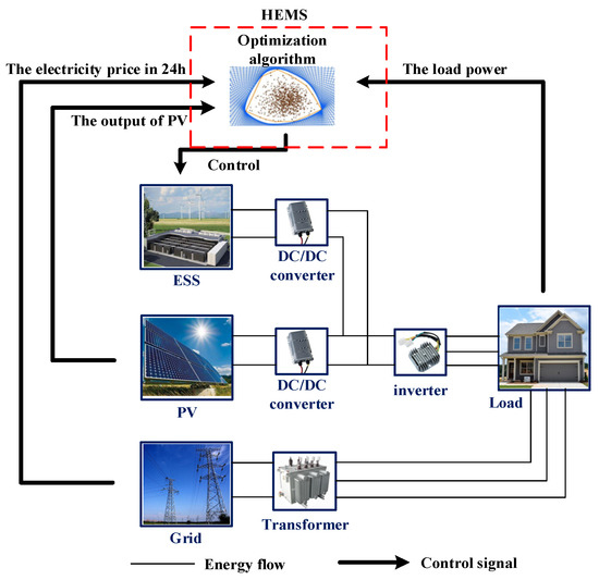
Figure 1.
The structure of PV-ESS.
In this study, only the types of ESSs in household PV-ESS systems are discussed. Regarding ESS, Abbassi A et al. conducted an analysis and economic comparison of the efficiency and the connection of the existing energy storage equipment to the power grid. The performance of various energy storage components can be represented by radar charts, as shown in Figure 2 [37,38].
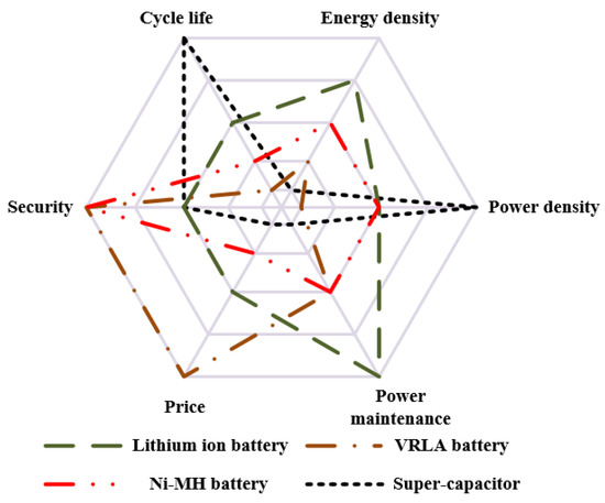
Figure 2.
Energy storage element performance comparison.
Battery energy storage is a common choice when PV power generation is equipped with energy storage systems. Its flexible capacity, power characteristics, and relatively compact size can be applied to various distributed systems. According to Figure 2, among several energy storage batteries, lithium-ion batteries can better meet the requirements of the demand side. However, during the operation of lithium-ion batteries, due to the particularity and instability of PV output, the working state is often complicated. This irregular charging and discharging behavior will lead to accelerated degradation of lithium-ion batteries, which will damage the durability and safety of the system to a certain extent. Additionally, with the development of lithium-ion batteries in recent years, their energy density has increased, their cost is constantly reduced, and the vigorous development of the new energy industry, resulting in the combination of distributed energy storage and new energy technology, has become a new technology route. The cooperation of energy storage systems and photovoltaic power generation systems can effectively alleviate the intermittence and instability of photovoltaic output. In the selection of energy storage system components, the cycle life of lithium-ion batteries needs to be further improved. Because of its high power density and long life, a super-capacitor–battery hybrid energy storage system becomes a reasonable scheme. Therefore, this study considers the use of lithium-ion batteries with SC and evaluates the feasibility of composite energy storage systems.
2.1. Modeling of PV-ESS System
2.1.1. Modeling of PV Module
PV cells have similar P-N junction structures. Under its electric field, the circuit is connected to generate current. A PV array is formed by connecting multiple solar cell modules in series and parallel [39,40]. The output power of the PV module is:
Here, PPV is the PV output power, kW; ηconv is the DC/DC converter efficiency; ηPV is the PV panel efficiency, it represents its ability to convert sunlight into electrical energy, %; S is the photovoltaic area, m2; It is the incident solar radiation at time t, W/m2. It should be noted that the size of the studied PV system is based on the unit kWp, and the actual PV system size can be obtained by multiplying the efficiency of the PV panel by solar radiation.
2.1.2. Modeling of ESS
Considering the accuracy and complexity of the model in the long term, the battery Rint equivalent circuit model is selected for the lithium-ion battery. The battery current Ibat can be obtained as:
The operating cost of the battery is the cost incurred by its irregular charging and discharging during operation, which in turn causes battery degradation. After conducting several experimental studies on the degradation process of LiFePO4 cells, Wang et al. proposed a semi-empirical model for estimating the battery capacity degradation as follows [41]:
Here, Qloss is the battery capacity degradation, Crate is the absolute value of the battery charge and discharge current rate, R is the ideal gas constant, Ea is the activation energy, A0 is the pre-exponential coefficient, Ah is the ampere–hour (Ah)-throughput, B is the third undetermined coefficient, z is the second undetermined coefficient, and Tbat is the temperature of the battery in Kelvin. Note that this model is based on the Arrhenius degradation model, wherein the effects of different charge and discharge rates, temperature, and charge and discharge power are considered.
Equation (3) can be rearranged as follows:
Next, finding the derivative of Ah in Equation (3) yields the following.
By introducing Equation (4) into Equation (5), it can obtain:
Here, Qloss,t+1 and Qloss,t denote the degradations of the battery from time t to time t + 1, respectively, and ΔAh is the accumulated A–h throughput of the battery during the same time period, determined as follows. For SC, the open circuit voltage USC of SC has a linear relationship with its state of charge SOCSC.
Normally, when SOCSC is less than 50%, it will not be used further unless it is charged. This is because the power contained in the SC is represented by the following equation.
Here, QSC is the energy released when SC discharges to SOCSC, CSC is the capacity of SC, and USC_max is its maximum voltage. When SOCSC is 50%, the SC will release 75% of the energy.
2.1.3. Modeling of Converter
The converter is an important part of the PV-ESS system and is the key factor affecting the economy of the system. From the user’s point of view, economy, high efficiency, reliability, and service life are the main requirements for the inverter. Because of the randomness, instability, and other characteristics of the PV output, it is necessary to employ a bidirectional DC/DC converter between the PV system and ESS to control the stability of charging and discharging, extend the life of the battery, and ensure the reliability of the system. Therefore, a high-power DC/DC converter is required.
The density and efficiency, the control mode and the structure should be relatively simple to improve the stability and service life of the system. During the PV-ESS system operation, the output power of each component is determined by Equation (9).
Here, ξconv_DC and ξconv_AC are 0/1 variables, which are determined by the connection between system components.
3. The Proposed Optimal Operation and Optimal Sizing of the PV-ESS System
The framework proposed in this study is shown in Figure 3, which can be roughly divided into two stages and five parts. In the first stage, by importing historical data, the theoretical optimal load scheduling solution is obtained based on dynamic programming (DP), and the optimal component size is obtained by comparison. Then, the outputs of each component are discretely characterized to obtain their output characteristics and to utilize the potential of the system. Additionally, in the second stage, based on the weather/load forecast and the result of the one-stage, by adjusting the weights of the objective functions in the MPC control algorithm, the output of the system components is controlled. The proposed study is implemented in the MATLAB environment, and the differential evolution algorithm (DE) is used to solve the proposed problem. Finally, periodically replace the original dataset with the newly generated system data.
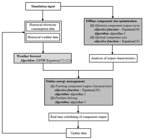
Figure 3.
The optimization framework of the PV-ESS system.
3.1. First-Stage
3.1.1. Objective Function and Constraints
The proposed PV-ESS system component sizing optimization framework is based on obtaining the average daily electricity savings under different system configurations and its comparison. The average daily electricity savings are obtained from the comprehensive system cost and the electricity fees required before and after optimization, as shown in Equation (10).
Here, Pgrid is the transmission power measured by the power grid at the current time, and it can be divided into two states according to whether the system has PV-ESS. Δt is an optimization interval of the optimization problem; λ and λann are the unit price and the average unit price of the corresponding item, which are obtained by conversion from the discount rate model; S is the size of the corresponding component. The model divides the total system cost into average purchase cost, daily average operation and maintenance cost, power purchase cost, and real-time battery degradation cost. However, the use of a stepped tariff can help achieve peak load cutting and valley filling, maintain the stability of the power system, and encourage users to form energy-saving habits. The Harbin Power Grid Corporation of China determined the electricity price as CNY 0.51/kWh. To account for the impact of electricity price, the stepped tariff used in reference [42] was selected for comparison with Harbin’s electricity price. The stepped tariff is processed to meet Equation (11).
Here, λa and λb are the fixed tariff and the stepped tariff, CNY/kWh; β is the adjustment ratio, which is the ratio of the sum of the two electricity prices in one day. When using a stepped tariff, the sum of the two different electricity prices in one day is equal. The adjusted electricity price is shown in Figure 4.
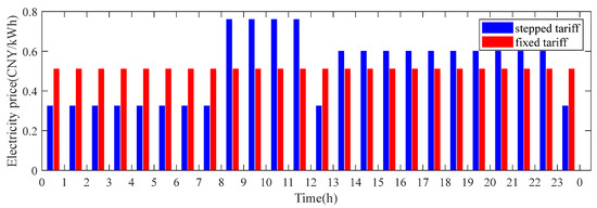
Figure 4.
Two electrovalence models after adjustment.
According to Figure 4, the stepped tariff varies greatly during different periods, among which the high electricity price periods are concentrated in the intervals 8:00~11:00, 17:00~22:00, and other peak consumption periods. Compared with the fixed tariff, a certain capacity of ESS can reduce the system operation cost by charging during the low electricity price period and supplying power to the load during the high electricity price period. Therefore, the objective of this study is to minimize electricity saving by minimizing the system purchase sharing cost, battery recession cost, and power purchase cost, and thereby obtain the optimal system capacity configuration under various constraints. The optimal capacity configuration of the system (OCS) is:
Here, i, j, k represent the size component serial number, which corresponds to components of different sizes; CPV(i) is the optimal PV capacity, kWp; Cbat(j) is the optimal lithium-ion battery capacity, kWh; CSC(k) is the optimal SC capacity, kWh. Additionally, in the process of system operation, the following constraints need to be met. During system operation, the following constraints should be met.
- (1)
- Power balance constraint
Here, Pload(t) on the left side of Equation (14) is the power required by the load, kW. On the right is the sum of photovoltaic power generation power PPV(t), grid side transmission power Pele(t), lithium-ion battery output power PBat(t), and supercapacitor output power PSC(t), kW.
- (2)
- Capacity constraint of ESS
SOCbat(t) and SOCSC(t) are, respectively, the SOC of battery and SC at time t, %. The capacity constraint of ESS is mainly determined by the SOC of the previous stage of ESS and the current charge–discharge capacity contraction.
- (3)
- Power constraint of ESS
The power constraint of the ESS is used to set the available charge and discharge capacity of the lithium-ion battery and supercapacitor, respectively, during system operation. The power constraint for ESS is given in Equation (16).
3.1.2. Optimization Framework
Based on the proposed cost model, the DP algorithm is used to calculate the optimal operation trajectory of each component of the system first. Thereafter, the theoretical optimal size of the system is obtained through comparison to maximize the system potential. The DP algorithm is a traditional and mature optimization algorithm. Compared with other algorithms, DP can obtain accurate global optimal solutions. Combined with the research objectives, the reverse order optimization process is provided in Algorithm 1.
| Algorithm 1: The optimization framework based on DP. |
| input: The PV-ESS parameters, aggregate of different component sizing systems, initial state of the system, simulation time interval, and length. |
| 1 repeat |
| 2 for each component size system do |
| 3 Divide the stages: Ts = 1 h |
| 4 Identify initial SOC of the ESS: 55% |
| 5 Identify state variable and decision variable: SOCbat and Pbat 6 Build the state transition function: 7 Build the evaluation function: 8 for each optimization interval 9 Optimize in reverse order 10 Update the state of the system 11 Save minimum objective function 12 end 13 Compare and analyze each electric cost 14 Update the optimal capacity allocation based on the minimum objective function 15 end 16 until The simulation length is reached output: The power curve of each component, the optimal component size in theory. |
Here, Cbat is the capacity of ESS in kW; Φt is the electricity saved by deciding Pbat from time t to time t + 1; φt is the maximum electricity saved by the system from time t + 1 until the end. By the hierarchical processing of the proposed method and according to the states before and after each optimization interval during the system operation, the scenarios corresponding to different decisions can be obtained. Thereafter, the theoretical optimal solution of load dispatching can be obtained.
3.2. Second-Stage
3.2.1. The PV Output Prediction Based on Long Short-Term Memory (LSTM)
For the PV prediction model in the proposed framework, LSTM, as a special recurrent neural network (RNN), can selectively input and remove information by introducing “gate operation”. It can not only process short-term information but also handle long-term dependence, thus enabling the overall network to process sequence-changing data and solve gradient disappearance and gradient explosion problems during long sequence training, as shown in Figure 5.
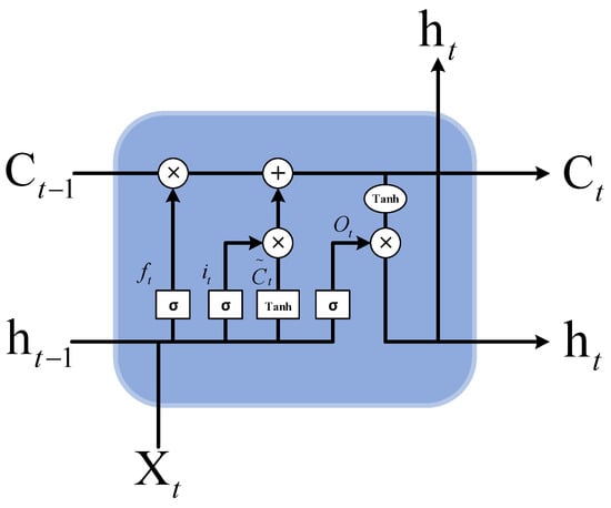
Figure 5.
LSTM internal unit structure.
When data flow into the LSTM unit, according to Equation (17), the forgetting gate reads the hidden layer state ht−1 and the last external input xt, multiplies the weight values, and outputs Wf. Finally, the sum of the superposition with the offset value bf is input into the activation function σ, and the probability of retaining the previous state ft is obtained as a result. According to Equation (18), the probability of keeping the new state is determined by the input gate it. Equation (19) provides the neuron candidate state, which is used to calculate the reserved part of the old state and the selected part of the candidate state so as to obtain the final state Ct of the current neuron. The output gate determines the output of the neuron and calculates the output hidden layer state ht from Equations (21) and (22). In this study, the learning rate is set to 0.001, epoch to 250, and dropout to 0.2. RMSE is used as the loss function.
3.2.2. The Dispatch Strategy Based on MPC
Because of the large amount of calculation, online application of DP is not easy. Although the optimal power flow between system components and the theoretical minimum operating cost of the system can be obtained, the full potential of the system cannot be exerted because of the inconsistent power flow between the two systems caused by the absence of real-time control. Therefore, an online control algorithm should be used to schedule the power flow among system components in real-time so that the system is robust. MPC solves a finite time domain optimization problem online using the current measurement information at each sampling time. It applies the first element of the obtained control sequence to the controlled object and repeats the above process at the next sampling time to refresh and solve the optimization problem. According to the linear discrete state space model:
Here, [PESS(k) Pcut(k) Pgrid(k)]T is the state vector, representing the real-time output power of each component in the system; [ΔPESS(k) ΔPcut(k) ΔPgrid(k)]T is the control variable vector; [rESS(k) rcut(k) rgrid(k)]T is the system disturbance caused by prediction error. The optimal output value of each component in the future finite time domain can be obtained through rolling optimization, as shown in Equation (23).
Here, Pu(k + i|k) represents the state variable of each component obtained in the k + i phase through prediction in the k phase; Δxu(k + i|k) represents the output increment of each component in the corresponding period; N is the total number of periods in the prediction time domain. Considering the particularity of the studied problem, the objective function is set as follows:
According to Equation (25), the objective function is temporarily divided into three terms: electricity price adjustment, battery power output, and battery power change rate term. Through follow-up, the optimal output status of each system component can be analyzed. The equation and the weight of each term can be adjusted to obtain the online energy management strategy. The proposed scheduling framework algorithm is provided in Algorithm 2.
| Algorithm 2: The Dispatch strategy based on MPC. |
| Input: The PV-ESS parameters, optimal components sizing in theory, initial state of the system, PV output prediction results, simulation time interval and length. |
| 1 repeat |
| 2 for each prediction interval do |
| 3 identify the initial state of system components |
| 4 build the output prediction model of each component: Pbat(k + 1) |
| 5 solve the rolling optimization problem based on DE (according to Section 3.2.2) 6 save the adjusted output sequence: Pbat(k + 1): 7 dispatch according to the first item of the optimization result sequence 8 time window backward 9 if (T ≠ Tmax) 10 then 11 continue rolling optimization 12 update the dispatch sequence 13 else 14 update the optimal prediction interval 15 end 16 end 17 until The simulation length is reached; output: The optimal prediction interval, the dispatch results of each component. |
3.2.3. The Model Solving Based on DE
Differential evolution (DE) is an intelligent algorithm based on population evolution and has the advantages of easy use, good convergence, and robustness. It is suitable for solving nonlinear and multivariable problems. The model proposed in Section 3.2.2 is solved using DE. According to the operation procedure of DE, the output sequence of ESS is taken in the finite time domain as the population individual. Each individual is expressed as:
Here, i is the number of individuals in the population sequence, representing the population size; G is the number of population evolution generations. At the beginning of the search for the optimal output curve, it is assumed that the initial individuals of the population obey the uniform probability distribution within the constraints. To increase population diversity, the crossover operator CR is introduced to perform crossover operations on the optimization population, as expressed in Equation (27).
For each population individual, the variation vector is obtained using Equation (28), where r1, r2, r3 is the sequence number of randomly selected individuals. The expansion of the population is controlled by the variation operator F.
In this study, the crossover probability is set to 0.9, the mutation probability is set to 0.4, the initial population number is set to 100, and the number of iterations is set to 200. To improve the probability of finding the optimal solution, the DE/rand-to-best/1/bin strategy is adopted for each generation of the population. Moreover, an adaptive mutation operator is introduced, as expressed in Equation (29).
The model solution framework based on DE is provided in Algorithm 3.
| Algorithm 3: The Model solving based on DE. |
| input: The PV-ESS parameters, prediction interval. |
| 1 initialize population |
| 2 calculate the fitness of each individual according to the fitness function |
| 3 if (failure, meet the termination conditions) |
| 4 then |
| 5 introduce adaptive mutation operator cross and variation 6 cross and variation 7 consider constraint condition 8 select the next generation population according to the objective function 9 else 10 output optimal individual 11 end 12 save the output sequence output: The optimal output sequence in a prediction interval. |
4. Simulation and Results
4.1. Meteorological Data and Load Profile
PV power generation is directly affected by temperature and seasonal changes. To reflect on the impact of climatic, seasonal variations, and other factors on the system capacity allocation, a case study of Harbin, China, was conducted. Harbin, Heilongjiang Province, China, is located between 125°42′~130°10′ E and 44°04′~46°40′ N, in the central region of Northeast Asia. As shown in Figure 6, there are four distinct seasons, with an average temperature of −19 °C in winter and 23 °C in summer. Precipitation is usually seen during the months of June–September. Due to these special climatic conditions, light intensity varies greatly in the four seasons.
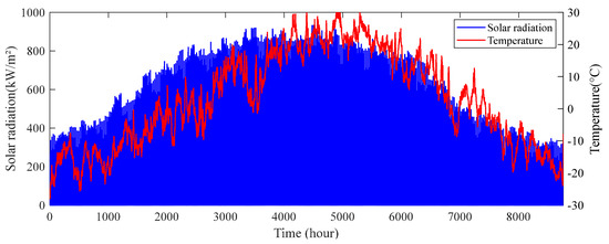
Figure 6.
Hourly average temperature and Solar radiation in Harbin.
The trends in solar radiation and temperature throughout the year are similar, indicating the direct impact of temperature on PV power generation and the importance of PV system capacity. When the changes in the residential load are small, a large-capacity PV system can meet the power demand in winter. However, PV power generation will inevitably be surplus in summer. On the contrary, a small-capacity photovoltaic system can meet the power demand in summer but cannot in winter. Furthermore, the parameters selected in this study are shown in Table 1.

Table 1.
Parameters of each component.
4.2. Simulation Results of the First-Stage
4.2.1. The Model Solving Based on DE
To prove the effectiveness of the proposed method, the PV-ESS system with sufficient capacity is first simulated, and the optimal output curve of each component is obtained, as shown in Figure 7.
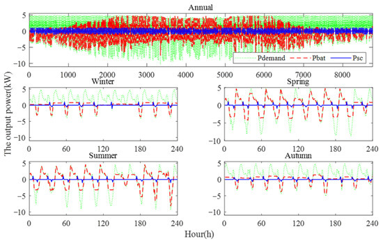
Figure 7.
The output curve of the components in the PV-ESS system.
Figure 7 shows the optimized annual output curve of the PV-ESS system when the PV capacity is 10 kWp, the lithium-ion battery capacity is 40 kWh, and the SC capacity is 2 kWh. Considering the seasonal changes, ten representative days in the four different seasons were selected for analysis. From the annual output curve of the system, it can be concluded that under the current capacity configuration, the PV-ESS system alone is not sufficient to supply the load demand. Most of the power gap is seen during autumn and winter. However, except for certain periods in summer, the ESS is able to absorb and use most of the redundant PV power generated.
By analyzing each component in ESS, it can be seen that the ESS can fully absorb the insufficient PV power generated during autumn and winter and release it during the period of power consumption. In terms of PV capacity, under the condition of constant daily load, excessive PV panels can be used to meet the power demand of the month under weak illumination intensity in winter; however, excess PV generation in summer is unavoidable. To avoid the wastage of resources, the ESS should absorb excess power. Conversely, a few PV panels are sufficient to meet the power demand in summer; however, in winter, the PV generation is insufficient. The proposed method considers the impact of irregular charging and discharging on the life of a lithium-ion battery and control its output to maintain constant current discharge during the discharge period. In the case of excess power generation, the proposed method can fully supply the system load when the available discharge capacity of the ESS is sufficient and conduct constant current discharge during other periods. Similarly, the charging rules can be determined based on the available charging capacity of ESS.
In addition, according to the system output curve of selected periods in different seasons, the system will predict the power required in the subsequent periods when the available electricity is sufficient. Thus, the charging and discharging of ESS can be controlled effectively. Based on the algorithm proposed in Section 3.1.2, the annual electricity cost savings of PV-ESS under two electricity price modes and different capacity configurations are simulated. The respective optimal capacity configurations are obtained through comparison. The simulation results are shown in Table 2 and Table 3.
Table 2.
The OCS of different components size of the system at a fixed tariff.
Table 3.
The OCS of different components size of the system at stepped tariff.
According to Table 2, when the system is at a fixed tariff, the optimal components sizes of the system are 8 kWp, 10 kWh, and 0 kW for photovoltaic panels, lithium-ion batteries, and SC, respectively. This indicates that the SC module cannot function effectively in this setting. The main reason is that, among the component sizes obtained, the lithium-ion battery has a large capacity, while the charging power of ESS is not more than 10 kW, which leads to an insufficient maximum charging rate of 0.5 C. The degradation cost of batteries under a relatively healthy working environment is small. Therefore, the ability of SC to smoothen the output power of the system is limited. The main function of SC is to smoothen the output from lithium-ion batteries. The other functions are similar to that of the grid, which makes it difficult for SC to function properly. In addition, the unit price of lithium-ion batteries differs greatly from that of SCs, so SCs bring small profits. The excessive redundant PV power generation can be consumed by configuring the battery with appropriate capacity. The system operation cost can be reduced if the redundant power generation is greater than the battery degradation cost.
In contrast, when the system is under stepped tariff, the optimal system capacity configuration obtained is 12 kWp, 25 kWh, and 0 kW. It indicates that the full advantage of ESS can be obtained using a stepped tariff. Due to the coupling relationship between system components, when the optimal size of the battery increases, a larger PV system is needed to match the requirements. ESS is always in an active state due to the differences in electricity prices. In addition, when the PV size is too small, and the PV generation capacity is insufficient, the SC module is in an empty state. Therefore, the battery degradation cost is far less than the average cost of SC.
4.2.2. The Model Solving Based on DE
The output characteristics of each component of the system should be analyzed to obtain a reasonable online energy management strategy. Discrete characterization is conducted according to the output of each component under the obtained optimal capacity configuration of the system. The SOC of the ESS when using fixed and stepped tariffs is shown in Figure 8.
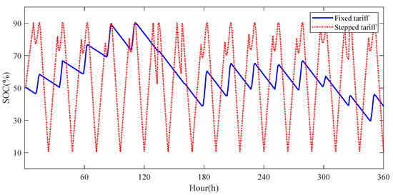
Figure 8.
Comparison of battery output of ESS under different electricity price mechanisms.
To clearly analyze the working rules of ESS in both cases, 360 h data were selected. The optimized output curve of ESS shows that it is in a constant current discharge state most of the time and maintains a constant current charge state when PV power generation is sufficient. This charge/discharge mode has little impact on the battery’s health. When the system is in fixed tariff, the overall trend of charging and discharging is unchanged, and the DOD of the battery is small. However, there are special scenarios where the charging and discharging capacity of the system is reserved. For example, in 0–180 h, although the PV power generation capacity is not enough to supply load demand, the ESS is generally in a charging state. In 300–360 h, ESS is always in a discharge state. This shows that the proposed method can effectively reserve available charging and discharging capacity in long time domains to save electricity costs and reduce battery degradation.
However, when the system is under stepped tariff, due to the large price difference, the system operation cost can be greatly reduced by purchasing power in the low price period and using it in the high price period. The electricity cost saved using this method is significantly greater than the cost incurred due to battery degradation. Therefore, the battery degradation of the system under a stepped tariff is greater than that under a fixed tariff. Moreover, it makes the charging and discharging curve of ESS under stepped tariff more regular; that is, charging and discharging with constant current according to the radiation conditions, by taking 24 h as a cycle. For the charging and discharging curves with high regularity, the rule-based energy management algorithm for online matching is usually used. Therefore, this study focuses on the discrete analysis of power flow in online energy management algorithms when the system is in fixed tariff, as shown in Figure 9.
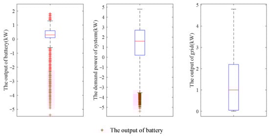
Figure 9.
The power discretization analysis of the system under fixed tariff (DP).
According to the results obtained, the output power of ESS in the discharge stage is around 0–1 kW, and the outliers are mainly distributed during the charging state of ESS. That is, the power fluctuation in its working range is small. In contrast, since the peak values of output power and power demand in the grid are similar, the grid plays a role in making up the power difference and smoothening the ESS output curve. In conclusion, according to the charging and discharging characteristics of each system component, the weight in Equation (24) is adjusted to simulate the theoretical optimal output curve of the system.
4.3. Simulation Results of the Second-Stage
4.3.1. Comparison of Prediction Results
Before model training, the annual unit photovoltaic output is taken as the overall sample set. The overall sample set is divided into a training set and a test set in the ratio 7:3. The data are then processed through data normalization and other operations. To avoid the cumulative error caused by the increase in prediction steps and to verify the model performance, the single-step prediction strategy is adopted for data set prediction. The MATLAB deep learning toolbox is used to simulate the LSTM. The simulation results are shown in Figure 10.
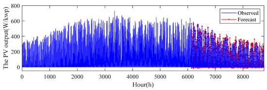
Figure 10.
The photovoltaic output prediction results under single input.
When the single input, single output prediction mode is adopted, the results can better track the PV output trend. However, the overall results still have large errors, and some of the predicted values are less than 0. To improve the prediction accuracy, the PV output and ambient temperature are simultaneously considered as the model inputs, and new prediction results are obtained.
According to the prediction results shown in Figure 11, it can be deduced that the prediction accuracy under multi-input is obviously higher than that under single input. Nevertheless, according to the RSME comparison results shown in Figure 12, it can be inferred that the proposed method can perfectly track future photovoltaic output. Although there are still some predicted values less than 0, its absolute values are small, which can be ignored and reset to zero when formulating online energy management strategies.
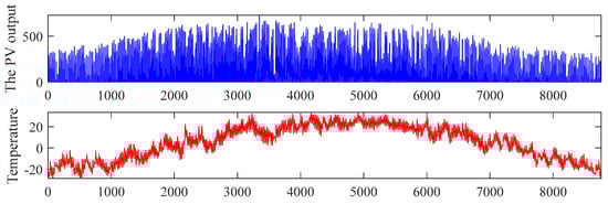
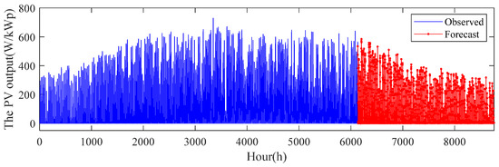
Figure 11.
The photovoltaic output prediction results under multi-input.
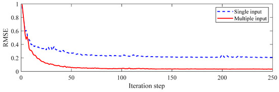
Figure 12.
The RSME comparison results.
4.3.2. Optimal Dispatch Strategy Based on MPC
Through the analysis of the output characteristics of each component during the system operation, Equation (25) can be adjusted and divided into four terms. The first two terms, respectively, represent the power consumption of the system and the attenuation of the ESS, the third term represents the impact of the reserved electricity in the ESS at the end of an expected interval on the subsequent optimization, and the fourth term represents the penalty for discarding PV power generation.
It should be noted that, for the proposed framework, if a prediction interval is too short, it cannot contain the operation rules of the system. If it is too long, it is subject to the accuracy of prediction data, and the problem easily falls into local optimization, yielding poor results. From the subsequent comparison and verification of simulation results, the prediction interval of 16–20 h seems better. The results are shown in Figure 13 and Figure 14.
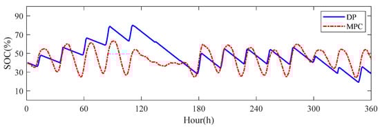
Figure 13.
Comparison of charging/discharging curves of DP and MPC.
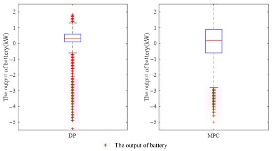
Figure 14.
Comparison of the power discretization analysis of DP and MPC.
Figure 13 shows the comparison of the SOC curves of ESS using the two algorithms when the weight coefficients in Equation (25) are 0.8, 1.2 × 10³, 1.1 × 10³, and 1.5 × 10⁴. From the results, the corresponding curve in the online energy management algorithm is smoother. In addition, due to the influence of the length of the prediction interval, the interval considered for each optimization calculation is only 16 h, which makes it impossible to identify the working characteristics of the system in the long interval, resulting in two curves which are not completely coincident. However, the trend is basically the same, indicating that the ESS generally works with the same rules. By combining the two box charts containing the annual system data, it can be concluded that the charging and discharging powers of the two algorithms are the same for most periods but diverge near the median. Moreover, the outliers of the online energy management algorithm used are more concentrated. The results show that, as far as power flow is concerned, its working mode is the same as the former and can be charged and discharged with constant currents for most periods. Even if the current charge/discharge rate is slightly higher than the previous period, it can still be timely adjusted in the subsequent periods, resulting in consistent total battery discharge, with only a slight increase in battery recession cost. The simulation results show that the algorithm can effectively simulate the optimal output curve of the system, and the saved electricity cost can reach 94.55% of the optimal result. It indicates that the proposed offline size optimization algorithm matches the online energy management algorithm, proving the effectiveness of the framework.
4.3.3. Influence of Different Climatic Conditions on Simulation Results
Based on the proposed PV-ESS component size optimization framework, this section considers four cities in China with representative climates as the research targets to explore the impact of climate on capacity allocation. The relevant data of the four cities are shown in Table 4.
Table 4.
Climate data of four cities.
According to Table 4, Harbin and Beijing have similar climates, and their average daily sunshine duration and power generation are almost the same. In both cases, the power generation in autumn and winter is much smaller than that in summer. In contrast, Chongqing and Sanya have higher temperatures throughout the year, but the rainy season is much longer than the first two cities, and the distribution of the rainy season is relatively average. From the perspective of power generation, Chongqing is the city with the lowest average daily power generation among the four cities. Although its annual temperature is relatively high, the sunshine duration is shortened due to rainy and foggy weather. Based on the proposed PV energy storage system module size optimization framework, the optimal capacity configuration of each of the four cities is obtained. The results are shown in Table 5 and Table 6.
Table 5.
Climate data of four cities at a fixed tariff.
Table 6.
Climate data of four cities at stepped tariff.
Although Harbin and Beijing have similar annual trends in temperature, sunshine, and other aspects, Beijing’s PV power generation capacity is slightly higher than Harbin’s, leading to increased PV panel configuration under the fixed tariff. Due to the strong coupling, the overall size of system components is increased, and the overall component size in Sanya is much larger than the first three. Apart from the strong coupling between components, the main reason is that the overall radiation intensity in Sanya is almost constant throughout the year and that the rainy season distribution is relatively average. When the system is in stepped tariff, due to the difference in electricity prices, the impact of power generation on the optimal component size is slightly reduced, resulting in a similar optimal component size in Harbin and Beijing. Moreover, the optimal system component size in Sanya is reduced, indicating that the proposed framework can accurately identify the working environment of the system and make adjustments.
In addition, according to Table 4, the proportion of power generation in the four cities is 1:1.04:0.66:1.21. Under the two different tariff mechanisms, the proportion of electricity charges that can be saved is 1:1.12:0.10:1.57 and 1:1.09:0.49:1.37, respectively. It can be concluded that under the fixed tariff, the proportion of electricity charges in Harbin and Beijing has not changed significantly. Sanya shows great potential for improvements in the PV energy utilization rate. On the contrary, results from Chongqing indicate that it is unreasonable to build a PV-ESS system in the urban area of the city. When the system is under stepped tariff, the proportion of electricity saved in Sanya is reduced from 1.57 to 1.37, which shows that the implementation of the stepped tariff mechanism can effectively save electricity bills in Harbin, Beijing, and other cities with four distinct seasons. In Chongqing, the implementation of a stepped tariff mechanism is more effective than the PV-ESS system configuration.
5. Conclusions
This study provides an optimization framework for the component sizing of the PV-ESS system based on HEMS. Unlike the previous studies, the proposed framework develops an online energy management strategy that matches the optimal capacity. During the operation of the system, full consideration is given to the uncertainty during operation, and the dataset is updated by combining day-ahead prediction and daytime scheduling to maintain accurate results. Considering the demand for energy storage components and the effectiveness of existing energy storage components, the lithium-ion battery/SC hybrid energy storage scheme was selected. Additionally, it has been proven that currently, SC is unable to leverage its own advantages, mainly because its functions are roughly the same as those on the power grid side.
By refining the optimization framework into two stages and five parts, the first stage can accurately identify the working characteristics of the system under the optimal system component size. Additionally, in the second stage, the online energy management strategy of the PV-ESS system was formulated by discrete characterization of the required power flow and multi-input LSTM prediction neural network. The proposed energy management strategy can accurately identify the working characteristics of the ESS and ensure that the ESS is in the optimal working state most of the time. The simulation results show that the strategy can effectively simulate the optimal output curve of the system, and the saved electricity cost can reach 94.55% of the optimal result. In addition, the simulation results show that the proposed method can account for the degradation of the BESS caused by irregular charging and discharging during the operation of the system. By reserving available space for charging and discharging, the battery can be maintained in a constant current charging and discharging state for as long as possible. Finally, considering the impact of climate factors on the results, four cities with different climate characteristics were simulated and compared, proving that the proposed framework can obtain the maximum potential of the system itself and maintain optimal economic efficiency. The proposed capacity optimization framework can be used to determine the size of the PV-ESS system in certain scenarios, such as residential and commercial buildings.
At present, research has not considered how to handle ESS with a partially depleted capacity. Therefore, future research will combine battery echelon utilization technology, combining batteries that have been used for a while with fresh batteries and applying them to more scenarios.
Author Contributions
Conceptualization, Y.L. and C.T.; methodology, Y.L.; software, Y.L.; validation, Y.L., C.T. and Y.Z.; formal analysis, Y.L.; investigation, Y.L.; resources, Y.L.; data curation, Y.L.; writing—original draft preparation, Y.L.; writing—review and editing, Y.L.; visualization, Y.L.; supervision, Y.L.; project administration, Y.L.; funding acquisition, C.T. All authors have read and agreed to the published version of the manuscript.
Funding
This research received no external funding.
Data Availability Statement
No new data were created or analyzed in this study. Data sharing is not applicable to this article.
Conflicts of Interest
The authors declare no conflict of interest.
References
- Hirsch, A.; Parag, Y.; Guerrero, J. Microgrids: A review of technologies, key drivers, and outstanding issues. Renew. Sustain. Energy Rev. 2018, 90, 402–411. [Google Scholar] [CrossRef]
- Bukar, A.L.; Tan, C.W. A review on stand-alone photovoltaic-wind energy system with fuel cell: System optimization and energy management strategy. J. Clean. Prod. 2019, 221, 73–88. [Google Scholar] [CrossRef]
- Ahmad, R.; Murtaza, A.F.; Sher, H.A. Power tracking techniques for efficient operation of photovoltaic array in solar applications—A review. Renew. Sustain. Energy Rev. 2019, 101, 82–102. [Google Scholar] [CrossRef]
- Jia, Y.T.; Alva, G.; Fang, G.Y. Development and applications of photovoltaic-thermal systems: A review. Renew. Sustain. Energy Rev. 2019, 102, 249–265. [Google Scholar] [CrossRef]
- Yang, D.; Kleissl, J.; Gueymard, C.A.; Pedro, H.T.; Coimbra, C.F. History and trends in solar irradiance and PV power forecasting: A preliminary assessment and review using text mining. Sol. Energy 2018, 168, 60–101. [Google Scholar] [CrossRef]
- Poompavai, T.; Kowsalya, M. Control and energy management strategies applied for solar photovoltaic and wind energy fed water pumping system: A review. Renew. Sustain. Energy Rev. 2019, 107, 108–122. [Google Scholar] [CrossRef]
- Hoque, N.; Kumar, S. Performance of photovoltaic micro utility systems. Energy Sustain. Dev. 2013, 17, 424–430. [Google Scholar] [CrossRef]
- Heinisch, V.; Göransson, L.; Erlandsson, R.; Hodel, H.; Johnsson, F.; Odenberger, M. Smart electric vehicle charging strategies for sectoral coupling in a city energy system. Appl. Energy 2021, 288, 116640. [Google Scholar] [CrossRef]
- Raghuwanshi, S.S.; Arya, R. Reliability evaluation of stand-alone hybrid photovoltaicenergy system for rural healthcare centre. Sustain. Energy Technol. Assess. 2020, 37, 100624. [Google Scholar]
- Mariano-Hernández, D.; Hernández-Callejo, L.; Zorita-Lamadrid, A.; Duque-Pérez, O.; García, F.S. A review of strategies for building energy management system: Model predictive control, demand side management, optimization, and fault detect & diagnosis. J. Build. Eng. 2021, 288, 101692. [Google Scholar]
- Wong, L.A.; Ramachandaramurthy, V.K.; Taylor, P.; Ekanayake, J.B.; Walker, S.L.; Padmanaban, S. Review on the optimal placement, sizing and control of an energy storage system in the distribution network. J. Energy Storage 2019, 21, 489–504. [Google Scholar] [CrossRef]
- Bayram, I.S.; Abdallah, M.; Tajer, A.; Qaraqe, K.A. A Stochastic Sizing Approach for Sharing-Based Energy Storage Applications. IEEE Trans. Smart Grid 2017, 8, 1075–1084. [Google Scholar] [CrossRef]
- Al-Ghussain, L.; Taylan, O.; Baker, D.K. An investigation of PV and wind energy system capacities for alternate short and long-termenergy storage sizing methodologies. Int. J. Energy Res. 2019, 43, 204–218. [Google Scholar] [CrossRef]
- Wang, Y.; Wang, B.; Chu, C.C.; Pota, H.; Gadh, R. Energy management for a commercial building microgrid with stationary and mobile battery storage. Energy Build. 2016, 116, 141–150. [Google Scholar] [CrossRef]
- Abbassi, A.; Dami, M.A.; Jemli, M. A statistical approach for hybrid energy storage system sizing based on capacity distributions in an autonomous PV/Wind power generation system. Renew. Energy 2017, 103, 81–93. [Google Scholar] [CrossRef]
- Sandhu, K.S.; Mahesh, A. A new approach of sizing battery energy storage system for smoothing the power fluctuations of a PV/wind hybrid system. Int. J. Energy Res. 2016, 40, 1221–1234. [Google Scholar] [CrossRef]
- Babacan, O.; Torre, W.; Kleissl, J. Siting and sizing of distributed energy storage to mitigate voltage impact by solar PV in distribution systems. Sol. Energy 2017, 146, 199–208. [Google Scholar] [CrossRef]
- Chaudhari, K.; Ukil, A.; Kumar, K.N.; Manandhar, U.; Kollimalla, S.K. Hybrid Optimization for Economic Deployment of ESS in PV-Integrated EV Charging Stations. IEEE Trans. Ind. Inform. 2018, 14, 106–116. [Google Scholar] [CrossRef]
- Abdelkader, A.; Rabeh, A.; Ali, D.M.; Mohamed, J. Multi-objective genetic algorithm based sizing optimization of a stand-alone wind/PV power supply system with enhanced battery/supercapacitor hybrid energy storage. Energy 2018, 163, 351–363. [Google Scholar] [CrossRef]
- Wang, C.; Yu, B.; Xiao, J.; Guo, L. Sizing of Energy Storage Systems for Output Smoothing of Renewable Energy Systems. Proc. CSEE 2012, 32, 1–8. [Google Scholar]
- Alhaider, M.; Fan, L.L. Planning Energy Storage and Photovoltaic Panels for Demand Response with Heating Ventilation and Air Conditioning Systems. IEEE Trans. Ind. Inform. 2018, 14, 5029–5037. [Google Scholar] [CrossRef]
- Erdinc, O.; Paterakis, N.G.; Pappi, I.N.; Bakirtzis, A.G.; Catalão, J.P. A new perspective for sizing of distributed generation and energy storage for smart households under demand response. Appl. Energy 2015, 143, 26–37. [Google Scholar] [CrossRef]
- Atia, R.; Yamada, N. Sizing and Analysis of Renewable Energy and Battery Systems in Residential Microgrids. IEEE Trans. Smart Grid 2016, 7, 1204–1213. [Google Scholar] [CrossRef]
- Khorramdel, H.; Aghaei, J.; Khorramdel, B.; Siano, P. Optimal Battery Sizing in Microgrids Using Probabilistic Unit Commitment. IEEE Trans. Ind. Inform. 2016, 45, 834–843. [Google Scholar] [CrossRef]
- Eltamaly, A.M.; Alotaibi, M.A. Novel Fuzzy-Swarm Optimization for Sizing of Hybrid Energy Systems Applying Smart Grid Concepts. IEEE Access 2021, 9, 93629–93650. [Google Scholar] [CrossRef]
- Alotaibi, M.A.; Eltamaly, A.M. A Smart Strategy for Sizing of Hybrid Renewable Energy System to Supply Remote Loads in Saudi Arabia. Energies 2021, 14, 7069. [Google Scholar] [CrossRef]
- Riana, A.D.; Jung-Su, K.; Hwachang, S. Suppression of PV Output Fluctuation Using a Battery Energy Storage System with Model Predictive Control. Renew. Sustain. Energy Rev. 2017, 17, 202–209. [Google Scholar]
- Ye, M.; Guo, H.; Cao, B. A model-based adaptive state of charge estimator for a lithium-ion battery using an improved adaptive particle filter. Applied Energy 2017, 190, 740–748. [Google Scholar] [CrossRef]
- Olaszi, B.D.; Ladanyi. Comparison of different discharge strategies of grid-connected residential PV systems with energy storage in perspective of optimal battery energy storage system sizing. Renew. Sustain. Energy Rev. 2016, 75, 710–718. [Google Scholar] [CrossRef]
- Korjani, S.; Casu, F.; Damiano, A.; Pilloni, V.; Serpi, A. An online energy management tool for sizing integrated PV-BESS systems for residential prosumers. Appl. Energy 2022, 313, 118765. [Google Scholar] [CrossRef]
- Wang, T.; O’Neill, D.; Kamath, H. Dynamic Control and Optimization of Distributed Energy Resources in a Microgrid. IEEE Trans. Smart Grid 2015, 6, 2884–2894. [Google Scholar] [CrossRef]
- Gupta, P.; Singh, R. PV power forecasting based on data-driven models: A review. Int. J. Sustain. Eng. 2021, 14, 1733–1755. [Google Scholar] [CrossRef]
- Carneiro, T.C.; de Carvalho PC, M.; Alves dos Santos, H.; Lima MA, F.B.; Braga, A.P.D.S. Review on Photovoltaic Power and Solar Resource Forecasting: Current Status and Trends. J. Sol. Energy Eng. 2022, 144, 010801. [Google Scholar] [CrossRef]
- Kumar, D.S.; Yagli, G.M.; Kashyap, M.; Srinivasan, D. Solar Irradiance Resource and Forecasting: A Comprehensive Review. IET Renew. Power Gener. 2020, 14, 1641–1656. [Google Scholar] [CrossRef]
- Erdener, B.C.; Feng, C.; Doubleday, K.; Florita, A.; Hodge, B.M. A review of behind-the-meter solar forecasting. Renew. Sustain. Energy Rev. 2022, 160, 112224. [Google Scholar] [CrossRef]
- Tawn, R.; Browell. A review of very short-term wind and solar power forecasting. Renew. Sustain. Energy Rev. 2021, 153, 111758. [Google Scholar] [CrossRef]
- Abbassi, A.; Gammoudi, R.; Dami, M.A.; Hasnaoui, O.; Jemli, M. An improved single-diode model parameters extraction at different operating conditions with a view to modeling a photovoltaic generator: A comparative study. Sol. Energy 2017, 155, 478–489. [Google Scholar] [CrossRef]
- Li, W. Framework of probabilistic power system planning. CSEE J. Power Energy Syst. 2015, 1, 1–8. [Google Scholar] [CrossRef]
- Moretón, R.; Lorenzo, E.; Pinto, A.; Muñoz, J.; Narvarte, L. From broadband horizontal to effective in-plane irradiation: A review of modelling and derived uncertainty for PV yield prediction. Renew. Sustain. Energy Rev. 2017, 78, 886–903. [Google Scholar] [CrossRef]
- De la Parra, I.; Muñoz, M.; Lorenzo, E.; García, M.; Marcos, J.; Martínez-Moreno, F. PV performance modelling: A review in the light of quality assurance for large PV plants. Renew. Sustain. Energy Rev. 2017, 78, 780–797. [Google Scholar] [CrossRef]
- Wang, J.; Liu, P.; Hicks-Garner, J.; Sherman, E.; Soukiazian, S.; Verbrugge, M.; Tataria, H.; Musser, J.; Finamore, P. Cycle-life model for graphite-LiFePO4 cells. J. Power Sources 2011, 196, 3942–3948. [Google Scholar] [CrossRef]
- Wu, J.; Xing, X.; Liu, X.; Guerrero, J.M.; Chen, Z. Energy Management Strategy for Grid-tied Microgrids considering the Energy Storage Efficiency. IEEE Trans. Ind. Electron. 2018, 65, 9539–9549. [Google Scholar] [CrossRef]


Disclaimer/Publisher’s Note: The statements, opinions and data contained in all publications are solely those of the individual author(s) and contributor(s) and not of MDPI and/or the editor(s). MDPI and/or the editor(s) disclaim responsibility for any injury to people or property resulting from any ideas, methods, instructions or products referred to in the content. |
© 2023 by the authors. Licensee MDPI, Basel, Switzerland. This article is an open access article distributed under the terms and conditions of the Creative Commons Attribution (CC BY) license (https://creativecommons.org/licenses/by/4.0/).