Abstract
This paper addresses the optimal stochastic allocation of distributed energy resources in distribution networks. Typically, uncertain problems are analyzed in multistage formulations, including case generation routines, resulting in computationally exhaustive programs. In this article, two probabilistic approaches are proposed–range probability optimization (RPO) and value probability optimization (VPO)–resulting in a single-stage, convex, stochastic optimal power flow problem. RPO maximizes probabilities within a range of uncertainty, whilst VPO optimizes the values of random variables and maximizes their probabilities. Random variables were modeled with hourly measurements fitted to the logistic distribution. These formulations were tested on two systems and compared against the deterministic case built from expected values. The results indicate that assuming deterministic conditions ends in highly underestimated losses. RPO showed that by including ±10% uncertainty, losses can be increased up to 40% with up to −72% photovoltaic capacity, depending on the system, whereas VPO resulted in up to 85% increases in power losses despite PV installations, with 20% greater probabilities on average. By implementing any of the proposed approaches, it was possible to obtain more probable upper envelopes in the objective, avoiding case generation stages and heuristic methods.
1. Introduction
The optimal power flow problem (AC-OPF) is an extensively used tool to find optimal operative set points in the planning and operation of power systems. Its framework is being transformed from a rigid, centralized setup, to a more flexible one by including new economic agents and operational strategies. For instance, with the introduction of peer-to-peer trading schemes, a consumer-producer (prosumer) is integrated into energy communities and the overall welfare of the community is optimized by coordinating resources and energy transactions with conventional grids [1], or the aggregation of distributed energy resources (DER) into multienergy virtual power plants, whose operation is economically optimized to provide services such as upstream reactive power support or frequency control [2]. Similarly, the problem of planning virtual microgrids (optimal partitions of a larger conventional distribution network) with the allocation of DER can be addressed with an integrated approach (instead of separating the problem) with the very same constraints imposed by the original AC-OPF [3]. Although the AC-OPF properly formulates a balanced steady-state problem for conventional networks, it has been also modified for the design of microgrids with Photovoltaic (PV) units and storage systems to overcome power intermittence from the utility to supply critical loads [4]. This increase in the number of applications for AC-OPF has been boosted by more efficient and cheaper technologies in the production of electricity (allowing consumers to meet part of their demand and sell surpluses); the integration of information technologies (IT) advancements in the operation within energy supply chain, and data science analyses (e.g., the implementation of IoT solutions for energy management in microgrids [5]; the aggregation of DER via IT [6]; the demand charcterization for infrastructure planning [7]; the statistical characterization of solar irradiation [8]; and solar predictions based on artificial neural networks [9]), requiring grid operators, especially in the distribution, to operate, considering uncertainties and multidirectional flows of power, currency, and information. Under these conditions, network planners and operators implement AC-OPF to optimize either individual or combined, technical, economical, or environmental objectives, such as power losses minimization [10], voltage regulation [11], emissions reduction [12], operational and infrastructure investment cost reductions [13,14], or a combination, resulting in techno-economic-environmental multiobjective formulations [15]. This requires the study of newer methodologies involving active distribution network modeling [16], adequate mathematical formulation of optimization problems aiming to increase efficiency and solution quality [17] and the proper implementation of optimization techniques to solve the problem [18]. Additionally, recent multidisciplinary research has been directed to increase computational efficiency in the solution of the OPF problem [18], showing results particularly in newer metaheuristic techniques (e.g., the arithmetic optimization algorithm (AOA) [19], the hybrid Harris hawks optimizer-AOA (hHHO-AOA) [20], and the mutation improved grey wolf optimizer (MIGWO) [21]), and in the convexification of the problem with relaxations based on second-order cones [22,23] or positive semi-definite expressions [24]. This is relevant since AC-OPF formulations are more complex than the original power balance problem; they might include nonlinear cost functions (in addition to the quadratic expression for the losses found in the original AC-OPF fomulation),mixed-integer expressions (as in, a reconfiguration [25] or resource allocation problem [26]), and/or uncertainty, which–individually or all together– are not necessarily convex when included to the problem (in addition to the non-convex quadratic constraints in the original AC-Power Flow problem), thus limiting the quality of the solutions and the scope of results. Nevertheless, if the necessary effort is made to make the problem convex, the solution is ensured to be optimal, unique, exact (if feasible), and solvable in polynomial time (if not combinatorial). If convex is not possible, suboptimal solutions are always obtainable with other tools (meta-heuristics), although the solution cannot be guaranteed to be exact or unique. However, such tools are particularly useful in such cases, as well as in multi-objective Pareto optimization [10].
Uncertainty has become relevant in the analysis of power systems, since most common DER technologies and demands have stochastic behavior. Uncertainty is typically included in optimization problems by implementing case analysis [11,27], Monte Carlo simulations [28], sensitivity analysis [29,30], or typically by using expected value reductions and treating the stochastic problem deterministically. Depending on the model used to describe uncertainty, the stochastic optimization problem can be formulated as a chance-constrained OPF, in which the knowledge of random variables is expressed by distribution functions, and their associated probabilities are constrained to comply with operational constraints, e.g., in [31], demand and PV are modeled with the normal distribution, and the probabilities constrain the problem to avoid voltage, line power flow, and storage power violations. In [32], the probability of frequency deviation violations constrains the primary frequency control problem. On the other hand, the optimization problem can be formulated in multi-stage approaches by generating representative cases that follow the distributions of random variables, and solving a deterministic problem for each case. For instance, in [16], a two-stage stochastic program is defined for load restoration in distributed microgrids, whose first stage generates the cases with Monte Carlo simulations, then reduces them using hierarchical clustering. This information is fed to the second stage, which implements AC-OPF to retrieve the solution set for each case. Similarly, in [33] two optimization stages are proposed, but for the first stage, uncertainty is modeled by implementing probability distributions, and scenarios are generated with the scenario tree method then reduced with the Kantorovich distance method. A different approach for the two-stage stochastic optimization can be seen in [34], in which for both stages, Monte Carlo sampling is implemented individually. See also [35] for a review in multiple techniques to handle uncertainty.
In contrast to the two stage stochastic programs, in this paper, two single-stage approaches are proposed to formulate convex stochastic AC-OPF problems regarding DER sizing and location. The allocation problem aims to install a single DER unit (photovoltaic PV) to minimize power losses in the system, considering demand and irradiance random variables that are modeled from measured data fitted to the logistic continuous distribution. With the implementation of proposed approaches it is intended to observe the effect of uncertainty on the planning of DER installations, and to provide methods that recollect high quality solutions, with fewer software implementations, within higher probability scenarios based on available data. The main contributions of this work are summarized as follows:
- The implementation of single-stage convex stochastic programs that require no additional software implementations, whose results are expected to be global optimum.
- The modeling of uncertainty using a probabilistic approach, based on data available. Its implementation in the optimization problem is performed with continuous logistic distribution functions. With this approach, other distribution functions can be used to calculate probabilities, as long as they can be formulated as concave expressions. With this, the formulation of the optimization problem is more flexible to different probability distributions that might better fit the data.
- The implementation of mathematical expressions for probabilities tailored to follow the sense of the optimization and the nature of the random variable.
- The results, showing that the deterministic case (based on expected values) represent a less likely case. On the other hand, both proposed approaches are more likely, thus better estimating the long-term expected behavior.
After this introduction, the rest of the manuscript is organized to present the notation first, followed by the formulation of the proposed optimization problems, an overview of the test systems (one of the systems implements a real-world model from a distribution network in San Andres Island in Colombia), and a summary of the resulting AC-OPF problems (deterministic and stochastic) with the computational implementation. Then the results, the discussion, and the conclusions are presented.
2. Methods
In this section, the notation used throughout the article is firstly described, followed by the formulation of nonconvex AC-OPF and a convex reformulation. Then, the proposed definition of the objective function regarding power losses and probabilities and, subsequently, constraints regarding the formulated PV-capacity-irradiance interface are defined. Finally, an overview of the deterministic and the proposed stochastic problems is shown together with the specifications in the computational implementation.
2.1. Notation
A distribution network consisting of the node set , and the set of lines , whose elements consist in a pair of nodes , can be represented as an undirected graph . The reference parameters are defined for the first node (busbar) of the system, which also hosts the main generator injecting the apparent power to supply the demand and cover the losses. Node is a neighbour of node if the pair are connected through a line whose complex admittance, , remains constant. The neighbourhood of the node , is the set of neighbouring nodes . The admittance matrix (size is ) of the network is composed of each line admittance in the neighbourhood (shunt admittances are ommited). Its diagonal elements are calculated with , while the off-diagonal elements are calculated with . The ∗ operator stands for the complex conjugate. The complex voltage is denoted as v. The squared magnitude of the voltage is represented by the variable u, while for two adjacent nodes , the product between and is represented with . The Euclidean norm is represented with the operator . The symbols and stand for the upper and lower bound, respectively. For multiperiod analyses, the set is introduced to extend the size of affected variables, i.e., for the h period of analysis. In this study, multiperiod analyses were carried out in hourly steps within a day. Probabilities are assigned to the letter p. In the optimization problems, stands for the objective function. Additional variables and symbols are presented throughout the paper and are explained as they appear. The bolded expression represents a row vector of ones, whereas represents the transpose of the row-vector of ones (column vector of ones). The functions and extract the real and imaginary components of the complex input argument.
2.2. AC-OPF Formulations
The AC-OPF problem is, as originally formulated by Carpentier, a nonconvex Quadratically Constrained Quadratic Program QCQP [36] (omitting objective function definition) since the admittance matrix is not Hermitian. The balance of power can be expressed as in Equation (1).
An alternative formulation can be implemented by taking advantage of the sparsity in the incidence matrix of radial networks. The Bus Injection Model (BIM) considers the current flow through each line (sending and receiving flows) connected to the node, as can be observed in Equation (2) [37]. This formulation continues being nonconvex.
As can be observed, in Equation (1), the sum takes into account each element within the admittance matrix, whereas in Equation (2), summation is only performed for each line in the neighborhood of the node with its respective admittance (it does not consider the admittance matrix, but single element admittance).
To convexify the problem, as proposed in [38] (See [22,39] for more comprehensive information regarding convex relaxations), a linearization is implemented by substituting quadratic expressions with affine ones, and relaxing the equivalent term to form second-order conic constraints. The linearization takes place by introducing a new complex variable that replaces quadratic voltage terms, as seen in Equation (3). From these relaxations, convexity can be ensured as long as the convex feasible set lies within the non-convex feasible set.
If one builds a matrix W with every element, it is possible to see that W must be hermitian, and the diagonal elements correspond to each node’s squared voltage magnitude. To the diagonal elements of W, a new variable u is assigned. These transformations can be observed in Equations (4)–(8), where the index i is replaced by the index k to leave the i as the imaginary unit.
These transformations are used to create a set of conic constraints (one for each line) taking advantage of the Euclidean norm of complex numbers (Equation (9)) and creating a separated expression for the term (Equation (10)). Combining those equalities, and relaxing them into inequalities, the set of convex conic constraints, namely second-order conic constraints (SOC), is expressed as in Equation (11).
The basic convex AC-OPF based on the BIM is then formulated as in Equation (12).
If a multi-period analysis is carried out, the relaxed AC-OPF formulation changes to the expressions in Equation (13).
Additional operational constraints can be included in the formulation, i.e., voltage limits, generator capacity, and line power flow limits, but in this paper, such restrictions are not considered because uncertainties could make the problem infeasible. Nevertheless, the generation in the reference node is only bounded to be non-negative, as expressed in Equation (14).
2.3. Objective Function
Now that the AC-OPF is constrained to convex terms, the objective function must be defined with convex expressions as well. Therefore, a single objective function is defined for two objectives: minimize power losses and maximize probabilities.
2.3.1. Energy Losses
The expression for Energy losses is typically nonconvex, but by using the aforementioned transformations, it is now convex (affine), as shown in Equation (15).
2.3.2. Probabilities
In this paper, the maximization of probabilities for the logistic probability distribution is carried out. The continuous logistic distribution is a two-parameter distribution, and has both probability density (pdf) , and cumulative probability (cdf) functions, whose definitions are shown in Equations (16) and (17), respectively.
The first proposed approach to handle uncertainty is called range probability optimization (RPO), and is defined as finding the value x of the random variable X within an uncertainty range by maximizing its probability of occurrence. Therefore, the maximization of this probability is included in the objective function. To calculate the probability for the random variable following the RPO approach, the cdf is implemented as depicted in Equation (18).
where and define the uncertainty range in which the probability is evaluated, and is the parameter that establishes the half width of the allowed uncertainty. The expression in Equation (19) results from the simplification of Equation (18), and after natural logarithm is applied, it is converted into a sum of concave expressions, as it is shown in Equation (20), which are convenient for maximization. The natural logarithm is a monotonically increasing function; thus, the maximization of the probability’s logarithm represents the maximization of the probability itself.
Besides the RPO, a different approach named value probability optimization (VPO) is proposed. It includes in the objective function the maximization of the random variable value and its probability of being greater than the value, as described in Equations (21)–(23), and the minimization of the value with the maximization of the variable’s probability of being less or equal than its value, as described in Equations (24) and (25).
After simplifications in Equation (23) and by applying the natural logarithm to it and to Equation (25), the resultant concave expressions are shown in Equations (26) and (27).
Since the aim of these formulations is to increase probabilities and decrease power losses, the random variables and the calculation of their probabilities must be assigned properly when considering VPO analyses. Generally speaking, if one is determined to reduce power losses, the demand is to be reduced either by managing it directly with demand response schemes or curtailment, or by supplying it with distributed resources. Consequently, and to avoid triviality in the solution, the demand coefficient is minimized and its probability maximized, following Equation (25), whereas the irradiance coefficient and its probability (Equation (22)) are both maximized. Calculating probabilities otherwise would end in trivial solutions: if the probability for the demand coefficient is calculated with Equation (22), the maximum probability is obtained when the variable reaches its lower bound while minimizing the variable’s value, and if the probability for the irradiance coefficient is calculated with Equation (25), the maximum probability is obtained when the variable reaches its upper bound, while maximizing the variable’s value. Therefore, the demand minimization and its probability maximization are included in the objective function with Equation (27), whereas the maximization of the irradiance coefficient and its probability is included with Equation (26).
2.4. DER and Demand Modeling
In this article, the generation through photovoltaic DER (PV) and the demand are modeled as stochastic processes from real data. The research group Electric Machines and Drives (EM&D) at the National University in Bogotá, Colombia, worked on demand characterization from data collected from Distribution Companies. The collected data for demand was measured hourly from 2018 until 2020, whereas, the hourly irradiance (global solar irradiance) measurements were retrieved from the Colombian Institute of Hydrology, Meteorology, and Environmental Studies (IDEAM) for the period 2015–2018.
To obtain the distribution parameters for both variables, the data were fitted hourly to a logistic distribution. In Figure 1, the fitted parameters are illustrated (see Table A1 in the Appendix A for mean and scale parameter values).

Figure 1.
Logistic distribution fitted parameters.
Although the data for irradiance and demand was collected for different short periods, and the modeling of random variables is based on statistics, we cannot expect important changes in consumption dynamics or the irradiance in the region. Due to extraordinary circumstances (e.g., pandemics [40]), one can infer that the data would be fitted resulting in different parameters, but in the long run, the differences in the results would be marginal, specially for such a small location. In this framework, only consistent changes in demographics or economics [41] and the implementation of demand side management schemes (i.e., demand response) would lead to important changes in the probabilistic parametrization of the random variables and, thus, in the results.
Consequently, irradiance () and demand coefficients () replace the random variable X seen through Equations (16)–(27), and modulate the behavior of the PV generation and the demand, respectively. Although the demand is typically defined constant for each node in power flow analysis , in this article the demand through every node is regulated evenly by the random coefficient as described in Equation (28).
2.4.1. PV Location Modeling
The optimization problem in this article includes the allocation (size and location) of a PV unit in the system. The location is represented by a Boolean variable that indicates if a PV unit is to be installed in a node or not (Equation (29)), whereas the size of the PV unit is modeled to deliver active power modulated linearly by the irradiance coefficient () with a constrained capacity. The rated capacity of the PV unit can be fully utilized if the irradiance measures W/m2 (base value), although such level was not registered in the measurements. The linearized expression for the power delivered by the PV unit, including its location, is shown in Equations (30)–(32).
where the variables and represent the location of the PV, the modulated power and the effective power of the located PV unit, respectively, and the parameters and stand for the maximum number of PV units to be installed and their maximum capacity, respectively.
2.4.2. PV-Capacity–Irradiance Interface
The interface between the PV unit power , its capacity , and the irradiance is expressed in Equation (33). This interface is hereafter named PCI.
This non-linear expression is linearized using piecewise linear approximations. The variables and are sectioned in k and m equidistant points from their minimum until their maximum values, giving place to coefficients interpolating the sectioned values in each variable, as shown in Equations (34)–(36).
where and are the set of sectioned values for the PV capacity, irradiance, and the resulting modulated power, respectively. The set of is a special ordered set 2 (SOS2), for which only two adjacent values (in rows and columns) can be nonzero, and its whole sum is one (Equation (37)). To ensure that only two adjacent rows and columns can be nonzero, two additional SOS2 sets are defined (one set for rows, the other for columns) such that the sum of their values is also one, as observed in Equations (38) and (39).
2.5. Test Systems
For this article, the data of two distribution systems– The IEEE33-bus system (I33) and the modeled distribution network for the neighborhood “Juan 23” (J23), located in San Andres Island (Colombia)–parameterize the AC-OPF formulations. The J23 system was modeled from data provided by the EM&D research group. The I33 system has a total demand of 3715 kW and 2300 kVAr with 210.9876 kW power losses (see system data in [42]) with a rated voltage of 12.66 kV, whereas the J23 system, with 13.6 kV rated voltage, totals 1302 kW and 593 kVAr in demand and 31.30 kW in power losses (see system data in Table A2 in the Appendix A). Each respective rated voltage and 1 MW (for both systems) are used as base values. If a multiperiod power flow analysis (see Equation (13)) is carried out with the demand following the mean averaged hourly profile ( in Table A1), then the losses sum up to 1.51 MWh/day for the I33 system and 337.25 kWh/day for the J23 system. As can be observed in Figure 2, the I33 and J23 systems have radial and radial/ring configurations, respectively.
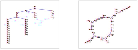
Figure 2.
Grid configuration of test cases: Left I33, right J23.
2.6. Deterministic AC-OPF Model
To set reference OPF results, the allocation problem is also considered deterministically. To carry this out, the mean profiles for irradiance and demand coefficients () will be included in the formulation to modulate demand and PV power injections. This model is much simpler than the stochastic one since the AC-OPF would not include the probability expressions in the objective function nor the PCI defined before, but only the PV location modeling. This model is described in Equation (44).
2.7. Stochastic AC-OPF Model
The formulation including objective function with Equation (20) (RPO) is intended to obtain the maximum probability values within a 10% uncertainty range, whereas AC-OPF with Equations (26) and (27) in the objective (VPO) is intended to find an operating point by minimizing the demand, and maximizing DER injections while maximizing probabilities in both random variables. Therefore, two OPF problems are defined (RPO and VPO), for two test systems (I33 and J23). The complete OPF, considering each case’s objective function and some additional operational constraints, is detailed in Equation (45).
2.8. Computational Implementation
The optimization problems defined in this article are implemented in CVXPY [43,44] through Anaconda’s Python distribution [45] and solved with MOSEK [46]. The following parameters (expressed in per unit) were implemented for the applicable simulation: , , , for , for . Solver parameters were kept in their default values.
3. Results
In this section, the main results obtained from the defined optimization problems are shown. For each system, the results for the deterministic AC-OPF problem are first outlined, followed by the results for the stochastic formulations (RPO and VPO), respectively. The RPO and VPO probabilities for the mean coefficients are available in Table A3 in the Appendix A. For each simulation, a table with its results (OPF) and power flow analyses is presented, where the PF() represents the results of a power flow analysis with the mean demand coefficents, and the PF() represents the results of a power flow analysis with the demand coefficents obtained from the stochastic OPF. For the deterministic problem, the OPF implements the demand and irradiance coefficients following the mean values, whereas for stochastic problems, the coefficients result from the optimization of their probabilities.
3.1. Results for the I33 System
3.1.1. Deterministic AC-OPF
An overview of the results of the AC-OPF formulated in Equation (41) for the I33 system is shown in Table 1.

Table 1.
Overall results of the deterministic OPF compared to multiperiod PF results for the I33 system.
It can be observed that, by implementing a PV unit on the system under mean conditions, the overall power losses are reduced a 31%. The voltage profile was also improved, by increasing the distance between the the lower voltage value and its lower bound. In practice, the system would comply if a 10% lower bound is defined, but if this constraint is tighten to the 5% lower bound, only the system with PV installation would not violate the limits. Computationally, the PF problem would be infeasible if the tighter constraint is included).
3.1.2. Stochastic OPF
Simulation results for the I33 test system under RPO (Equation (19) in the objective function) are summarized in Table 2. The demand coefficients’ profile and probabilities are depicted in Figure 3 while those of the irradiance coefficients profile and their probabilities are shown in Figure 4 (see Table A4 in the Appendix A for detailed hourly modulating coefficients and their associated probabilities).
Table 2.
Overall results of RPO-OPF compared to multiperiod PF results for the I33 system.
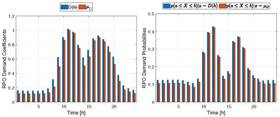
Figure 3.
Demand coefficients and mean values with RPO probabilities.
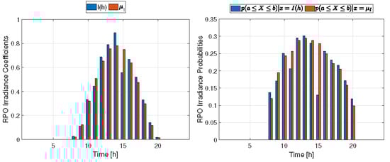
Figure 4.
Irradiance coefficients and mean values with RPO probabilities.
It can be observed that, by implementing a PV unit on the system considering uncertainty under RPO approach, the overall power losses are reduced a 6.5% compared to the mean power flow analysis with a reduced PV capacity of 11% compared the deterministic scenario, and a 20% reduction in losses compared to the power flow analysis with the obtained RPO demand coefficients. The voltage profile was also improved, although with RPO demand coefficients, the power flow analysis got closer the lower bound than with the mean PF.
For simulations under VPO (Equations (24) and (21) for demand and irradiance, respectively, in the objective function), results are summarized in Table 3 and detailed with coefficients and probabilities in Table A5. The demand coefficients’ profile and probabilities are illustrated in Figure 5 while those of the irradiance coefficients are depicted in Figure 6.
Table 3.
Overall results from VPO-OPF compared to multiperiod PF results for the I33 system.

Figure 5.
Demand coefficients and mean values with VPO probabilities.
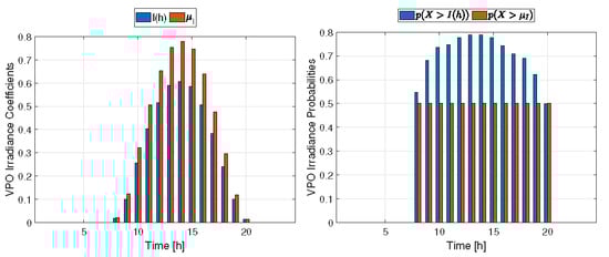
Figure 6.
Irradiance coefficients and mean values with VPO probabilities.
It can be observed that, by implementing a PV unit on the system considering uncertainty under VPO approach, the overall power losses are increased a 26% compared to the mean power flow analysis, and reduced a 27% compared to the power flow analysis with the obtained VPO demand coefficients. The voltage profile was also improved, although the PF analysis with VPO demand coefficients would not comply the 10% lower bound.
3.2. Results for the J23 System
3.2.1. Deterministic AC-OPF
An overview of the results of the AC-OPF formulated in Equation (41) for the J23 system is shown in Table 4.
Table 4.
Overall results of deterministic OPF compared to multiperiod PF results for the J23 system.
It can be observed that, by implementing a PV unit on the system under mean conditions, the overall power losses are reduced a 30%. The voltage profile was marginally improved.
3.2.2. Stochastic OPF
Simulation results for the J23 test system under RPO (Equation (19) in the objective function) are summarized in Table 5. The profiles outlined by demand coefficients and their probabilities are depicted in Figure 7, while the profiles for irradiance and probabilities are shown in Figure 8 (see Table A6 in the Appendix A for detailed hourly modulating coefficients and their associated probabilities).
Table 5.
Overall results from RPO-OPF compared to multiperiod PF results for the J23 system.
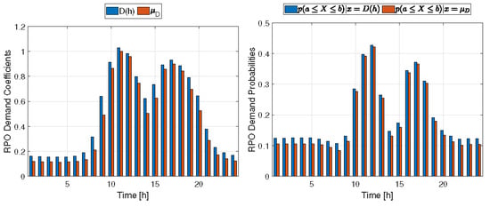
Figure 7.
Demand coefficients and mean values with RPO probabilities.
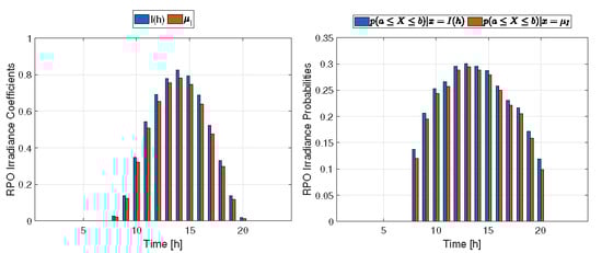
Figure 8.
Irradiance coefficients and mean values with RPO probabilities.
It can be observed that, by implementing a PV unit on the system considering uncertainty under RPO approach, the overall power losses are reduced a 20% compared to the mean power flow analysis, and a 31% compared to the power flow analysis with the obtained RPO demand coefficients. The voltage profile was marginally improved. Although the PF with RPO demand coefficients shows greater losses the the PF with mean coefficients, the capacity of the PV unit was reduced (72%).
For simulations under VPO (Equations (24) and (21) for demand and irradiance, respectively, in the objective function), results are summarized in Table 6 and detailed with coefficients and probabilities in Table A7. Profiles shaped from demand coefficients and their probabilities are illustrated in Figure 9 while the profiles constructed from irradiance coefficients and their probabilities are shown in Figure 10.
Table 6.
Overall results from VPO-OPF compared to multiperiod PF results for the J23 system.
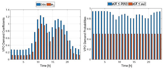
Figure 9.
Demand coefficients and mean values with VPO probabilities.
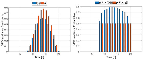
Figure 10.
Irradiance coefficients and mean values with VPO probabilities.
It can be observed that, by implementing a PV unit on the system considering uncertainty under VPO approach, the overall power losses are increased a 3.1% compared to the mean power flow analysis, and reduced a 30% compared to the power flow analysis with the obtained VPO demand coefficients. The voltage profile was also improved.
4. Discussion
For the I33 system, it could be observed from the results that the averaged probabilities during the day are increased by around 1.4% (RPO) and 35% (VPO) for demand, and by around 1.1% (RPO) and 20% (VPO) for irradiance, compared to the deterministic case. The location of the PV unit changed from node 8 to nodes 17 and 12 under RPO and VPO, respectively. Its capacity was kept near the upper bound in the deterministic and VPO cases, while it suffered an 11% reduction with the RPO, suggesting that even under uncertainty, DER units should be located in the most congested branch (the active power load is distributed to 11.57% in branch 2-6, 28.93% in branch 7-18, 9.69% in branch 19-22, 25.03% in branch 23-25 and 24.76% in branch 26-33). The minimum power loss was achieved in the deterministic case, followed by a 37% increase for RPO and a 85% increase for the VPO, approximately, showing how sensitive the analysis can be to uncertain values. Although demand and irradiance profiles suffered small deviations compared to the expected values, the system losses were affected much more negatively compared to the improvements gained in probabilities, even when deploying DER optimally.
The results for the VPO can be interpreted as an approximation to the worst-case scenario, since, as observed in Figure 5 and Figure 6, the obtained demand and irradiance coefficients are considerably higher and lower than the mean values, respectively, and both probabilities (to have lower demand and greater irradiance coefficients) are very high (>80% for demand and >70% for irradiance on average). In other words, the probability of the losses being less than 1.91 MWh/day is, on an hourly average, greater than 70%, compared to the 50% on hourly average that resulted from estimating the random variables to the mean values. In contrast to the RPO analysis, a drastic increase in power losses was accompanied with increases in probabilities compared with the deterministic case.
These results also allow for the analysis of other operating constraints, such as voltage magnitudes. It could be observed that the operational voltage limit constraint might be violated (especially the lower bound) when considering scenarios with worsened conditions, as in VPO, i.e., if the demand coefficients from VPO were considered for power flow analysis (without PV), the lower 10% bound would not be complied (see Table 3). However, the installation of the PV unit kept voltage magnitudes within the lower 10% bound. Evidently, tighter bounds in voltages might take the problem to infeasibility regions or, in a practical scenario, make the grid noncompliant to operative constraints under uncertainty, which might represent economic losses due to penalties.
For the J23 system, results were somewhat similar to the I33 ones. RPO and VPO probabilities increased by 1.4% and 38% for demand and by 0.9% and 21% for irradiance, respectively, compared to the deterministic case. This indicates that probabilities are not very affected by the system even though the random variables affect directly the power losses, which at the same time depends on the grid’s configuration and its parameters (size, redundancy, line impedances, load distribution, voltage level). As in the I33, the PV units were located in the most congested branch, in contrast to the deterministic case, in which they were located it in the second most congested branch (the active power load is distributed to 20.12% in branch 2-11, 35.71% in branch 12-25, 26.69% in branch 26-43 and 17.46% in branch 28-32). Regarding PV capacity, an important reduction happened when comparing both systems. In the I33 system, the PV capacity was kept capped, but in the RPO case, where it was reduced 11%, yet in the J23, PV capacity reached near the 40% of the maximum capacity in the deterministic case, and decreased under uncertainty to the 12% of the maximum with both RPO and VPO approaches.
Similar to the results for the I33 system, the J23 system gathered the minimum energy losses from the deterministic case, and progressively worsened under uncertainty (26% and 30% increases for RPO and VPO, respectively). Probabilities were increased likewise, as in the analyses for I33.
Regarding voltages, the J23 system had significantly lower losses than the I33 system in the power flow analysis (PF). This was also reflected in the voltage envelopes shown in the different OPF analysis, where the minimum voltage remained almost unaltered within the 1% range even in cases with greater demand and lower irradiance (VPO). This explains that the J23 grid has the capability to sustain greater loads under uncertainty, possibly with greater hosting capacities, while operating safely.
In Figure A1 and Figure A2 for I33, and Figure A3 and Figure A4 for J23 on the Appendix A, it is possible to observe how the probability of coefficient profiles under RPO and VPO is compared with the probability under the opposite approach, i.e., the probability of the demand and irradiance profiles obtained from RPO compared with the probability of those profiles under VPO, and vice-versa. The illustrations show that probabilities are greater when calculated with the profiles obtained from their respective analysis than with the opposite. However, for irradiance profiles, the differences between the probabilities are noticeable, especially when comparing VPO probabilities, indicating that RPO irradiance coefficients and mean values are overestimated, whereas the VPO profiles show lower RPO probabilities but establish a case with higher probabilities of being more favorable, since the range in which the random variable could fall is much wider. To summarize, mean value estimations have lower probabilities, resulting in important power loss underestimations, whereas under the RPO approach, a better estimation is obtained, even though the irradiance is clearly overestimated. Under the VPO approach, an even more probable case is defined by estimating worsened conditions for the objective, showing that both deterministic and RPO approaches underestimate the losses with conditions that are less likely.
Finally, the formulation of the proposed convex stochastic programs allowed us to obtain global optimal solutions. Although most of the variables in the proposed stochastic programs are integer, the problem size (directly related to the grid’s size) did not have any considerable impact on the solving time. On the contrary, for the I33 stochastic AC-OPFs, it took longer to find the solution. An explanation for this is that variations in the variables within the PCI (which contains the majority of integer variables and has the same dimensions for each test case), produce greater effects in power losses due to line lengths (impedance) and distribution of greater demands, requiring more intensive branch-and-bound steps, until the difference between the objective upper and lower bounds, set by the improvements in root relaxation and the incumbent solution,respectively, lies within the parameterized relative gap. On the other hand, the lower power loss levels present in the J23 system would indicate that a DC-power flow analysis can be a more adequate tool to analyze the system.
5. Conclusions
In this article, two alternatives are proposed to handle uncertainties on convex AC-OPF formulations, whose random variables are based on real measurements of demand and irradiance fitted to the logistic distribution. The effective PV power capability is related to the irradiance and to its capacity, by means of a nonlinear expression. To linearize it, a PV-capacity-irradiance (PCI) interface was implemented using piecewise linear approximations. One of the proposed approaches is called range probability optimization (RPO), and is used to maximize the probability of occurrence for random variables within a range of uncertainty, which is defined as a parameter (ϵ = ±0.1). The second approach is called value probability optimization (VPO), in which the values of the random variables are optimized along with the maximization of their probabilities. For the VPO to make sense, and to avoid trivial solutions, random variables and the probability functions are assigned following the sense of the main objective (minimize power losses). Thus, the demand is minimized while maximizing the probability of having lower or equal demand, and the irradiance is maximized while maximizing the probability of having greater irradiance. The proposed approaches were implemented for two distribution networks: The IEEE 33-bus test system and the modeled distribution network in the “Juan 23” neighborhood in San Andres Island (Colombia), and tested against the deterministic case, whose parameters follow the expected values of the distribution. The problem of allocating DER in distribution networks was modified to include uncertainty under RPO and VPO approaches, and as a result, it was possible to observe the problem’s sensitivity to uncertainty. With the RPO, although the variation in the averaged probabilities for the demand and irradiance coefficients was very small, and the location of the PV unit remained in the most congested branch, the capacity of the PV unit was decreased due to overestimated irradiance and underestimated demand, resulting in increased losses compared to the deterministic case. Meanwhile, with the VPO approach, by increasing the probabilities, the resulting profiles for demand and irradiance coefficients showed negative behaviors towards the minimization of power losses, suggesting that VPO approximates the problem to an scenario with worsened conditions without being the worst-case scenario, which provides robust information for stochastic decision making without underestimating (or overestimating) random variables, or over-sizing DER installations, as the worst-case scenario would suggest.
Regarding computational efficiency, the proposed stochastic formulations resulted in the collection of global optimal solutions due to convexity, and the inclusion of mixed-integer expressions hadn’t the expected impact on computation times for combinatorial problems, since systems with bigger size, i.e., J23, were actually solved faster, which is explained by a greater sensitivity of the objectives to the integer variables in systems with greater base losses and deviations in bus voltages, such as in the I33. This presents a disadvantage when implementing linearized formulations based on piecewise linear approximations, because, even though the problem is convex, the formulation is combinatorial, compromising scalability by requiring additional computation power. The trade-off between accuracy and computation times should be regarded when considering such implementations.
As future work, it is proposed to perform different RPO analyses varying the range width (ϵ), and test the VPO probability of the resulting irradiance profiles to see if the differences between both approaches can be narrowed. Considering that Energy Storage Systems (ESS) are usually implemented in power systems to overcome uncertainties in DER, it is proposed to test both VPO and RPO approaches in the allocation of DER and ESS resources, and test if ESS has effects on probabilities. Additionally, it can be interesting to assign different demand profiles following geographic demand characteristics in the network, to consider the implementation of demand response schemes or curtailment in the probabilistic model of the demand, and to fit the demand and irradiance data to other distribution functions to see its impact on the convexity of the formulations and on results themselves. Since the proposed formulations are convex MI-SOCP formulations, it can be interesting to find solutions using meta-heuristic techniques for each system, with convex and non-convex formulations, and see the differences in solution quality and computation times. Additionally, it is proposed to test the approaches on networks similar to the J23 (low losses) constrained to DC-power flow equations.
Author Contributions
Conceptualization, D.M.O. and J.R.G.; Methodology, D.M.O. and J.R.G.; investigation, D.M.O.; writing—original draft preparation, D.M.O.; writing—review and editing, D.M.O. and J.R.G.; funding acquisition, J.R.G. All authors have read and agreed to the published version of the manuscript.
Funding
This research was supported by Colombian Ministerio de Ciencia y Tecnología and Universidad Nacional de Colombia under grant “Becas del bicentenario, Corte 1: Formación de capital humano de alto nivel Universidad Nacional de Colombia” [BPIN:2019000100026] and Electrical Machines and Drives (EM&D) from Universidad Nacional de Colombia and Project Think Green on the island of San Andres [BPIN: 2016000100002 EEDAS ESP].
Data Availability Statement
Additional data are available on request by contacting the corresponding author of this manuscript.
Acknowledgments
The authors would like to acknowledge the contributions of the EM&D group to this article, particularly Alvaro Zambrano and Santiago Toledo for providing the San Andres demand characterization data and the J23 data for its modeling. We would like to thank Gustavo Bula and Eduardo Mojica at Universidad Nacional for the insightful conversations regarding convex optimization.
Conflicts of Interest
The authors declare no conflict of interest.
Abbreviations
The following abbreviations are used in this manuscript:
| AC-OPF | AC-Optimal Power Flow |
| AOA | Arithmetic Optimization Algorithm |
| BIM | Bus-Injection Model |
| CDF | Cumulative Probability Function |
| DER | Distributed Energy Resources |
| EM&D | Electrical Machines And Drives |
| GWO | Grey Wolf Optimizer |
| HHO | Harris Hawks Optimizer |
| hHHO-AOA | Hybrid HHO-AOA |
| I33 | IEEE 33-bus system |
| IDEAM | Instituto de Hidrología, Meteorología y Estudios Ambientales |
| IoT | Internet of Things |
| IT | Information Technologies |
| J23 | Juan 23 Distribution Network |
| MIGWO | Mutation Improved Grey Wolf Optimizer |
| MI-SOCP | Mixed-Integer Second Order Conic Program |
| PCI | PV-Capacity-Irradiance interface |
| Probability Density Function | |
| PF | Power Flow |
| PV | Photovoltaic Energy |
| QCQP | Quadratically Constrained Quadratic Problem |
| RPO | Range Probability Optimization |
| SOC | Second Order Conic |
| SOS2 | Special Ordered Set 2 |
| VPO | Value-Probability Optimization |
Appendix A
Table A1.
Fitted parameters of logistic distribution for demand and irradiance.
Table A1.
Fitted parameters of logistic distribution for demand and irradiance.
| h | ||||
|---|---|---|---|---|
| 1 | 0.1196 | 0.0567 | 0 | 0 |
| 2 | 0.1165 | 0.0551 | 0 | 0 |
| 3 | 0.1152 | 0.0541 | 0 | 0 |
| 4 | 0.1138 | 0.0534 | 0 | 0 |
| 5 | 0.1151 | 0.0541 | 0 | 0 |
| 6 | 0.1181 | 0.0573 | 0 | 0 |
| 7 | 0.1321 | 0.0704 | 0 | 0 |
| 8 | 0.2111 | 0.1248 | 0.0197 | 0.0082 |
| 9 | 0.4919 | 0.2152 | 0.1228 | 0.0311 |
| 10 | 0.8634 | 0.1519 | 0.3214 | 0.0646 |
| 11 | 1.0000 | 0.1208 | 0.5064 | 0.0963 |
| 12 | 0.9578 | 0.1064 | 0.6537 | 0.1102 |
| 13 | 0.7464 | 0.1427 | 0.7540 | 0.1243 |
| 14 | 0.5029 | 0.1902 | 0.7804 | 0.1315 |
| 15 | 0.6278 | 0.1950 | 0.7478 | 0.1304 |
| 16 | 0.8580 | 0.1220 | 0.6398 | 0.1256 |
| 17 | 0.8989 | 0.1170 | 0.4761 | 0.1060 |
| 18 | 0.8428 | 0.1346 | 0.2965 | 0.0713 |
| 19 | 0.6953 | 0.1918 | 0.1180 | 0.0370 |
| 20 | 0.5249 | 0.1938 | 0.0135 | 0.0068 |
| 21 | 0.2884 | 0.1268 | 0 | 0 |
| 22 | 0.1706 | 0.0833 | 0 | 0 |
| 23 | 0.1397 | 0.0669 | 0 | 0 |
| 24 | 0.1237 | 0.0592 | 0 | 0 |
Table A2.
J23 distribution network model data.
Table A2.
J23 distribution network model data.
| i | j | [MW] | [MW] | ||
|---|---|---|---|---|---|
| 1 | 2 | 0.16715 | 0.10971 | 0.03129 | 0.01425 |
| 2 | 3 | 0.03768 | 0.02472 | 0.03129 | 0.01425 |
| 3 | 4 | 0.01704 | 0.01118 | 0.03129 | 0.01425 |
| 4 | 5 | 0.02891 | 0.01897 | 0.02086 | 0.00950 |
| 5 | 6 | 0.01808 | 0.01186 | 0.03129 | 0.01425 |
| 6 | 7 | 0.02551 | 0.01674 | 0 | 0 |
| 7 | 8 | 0.01723 | 0.01130 | 0.04694 | 0.02138 |
| 8 | 9 | 0.02391 | 0.01569 | 0.03129 | 0.01425 |
| 11 | 10 | 0.01067 | 0.00700 | 0 | 0 |
| 7 | 11 | 0.02905 | 0.01906 | 0.03129 | 0.01425 |
| 10 | 12 | 0.01181 | 0.00775 | 0.03129 | 0.01425 |
| 12 | 13 | 0.01027 | 0.00674 | 0.04694 | 0.02138 |
| 13 | 14 | 0.01506 | 0.00988 | 0.04694 | 0.02138 |
| 14 | 15 | 0.02613 | 0.01715 | 0.03129 | 0.01425 |
| 15 | 16 | 0.00610 | 0.00400 | 0 | 0 |
| 16 | 17 | 0.00528 | 0.00346 | 0.03129 | 0.01425 |
| 17 | 18 | 0.00278 | 0.00182 | 0 | 0 |
| 18 | 19 | 0.01193 | 0.00783 | 0.04694 | 0.02138 |
| 19 | 20 | 0.00741 | 0.00486 | 0.04694 | 0.02138 |
| 16 | 21 | 0.00827 | 0.00543 | 0.04694 | 0.02138 |
| 23 | 22 | 0.21027 | 0.13798 | 0.04694 | 0.02138 |
| 18 | 23 | 0.03503 | 0.02298 | 0.04694 | 0.02138 |
| 23 | 24 | 0.01012 | 0.00664 | 0.03129 | 0.01425 |
| 24 | 25 | 0.00371 | 0.00243 | 0 | 0 |
| 25 | 26 | 0.02282 | 0.01497 | 0.02086 | 0.00950 |
| 26 | 27 | 0.01808 | 0.01186 | 0 | 0 |
| 25 | 28 | 0.01047 | 0.00687 | 0.04694 | 0.02138 |
| 28 | 29 | 0.01921 | 0.01261 | 0.04694 | 0.02138 |
| 29 | 30 | 0.00544 | 0.00357 | 0.01877 | 0.00855 |
| 29 | 31 | 0.00751 | 0.00493 | 0.06259 | 0.02850 |
| 31 | 32 | 0.00699 | 0.00459 | 0.04694 | 0.02138 |
| 27 | 33 | 0.00699 | 0.00459 | 0.04694 | 0.02138 |
| 27 | 34 | 0.03341 | 0.02193 | 0.03129 | 0.01425 |
| 37 | 35 | 0.00931 | 0.00611 | 0.03129 | 0.01425 |
| 35 | 36 | 0.01037 | 0.00680 | 0.03129 | 0.01425 |
| 34 | 37 | 0.01782 | 0.01169 | 0 | 0 |
| 37 | 38 | 0.00618 | 0.00405 | 0.03129 | 0.01425 |
| 38 | 39 | 0.01395 | 0.00915 | 0.02086 | 0.00950 |
| 39 | 40 | 0.00917 | 0.00602 | 0.04694 | 0.02138 |
| 40 | 41 | 0.02503 | 0.01643 | 0 | 0 |
| 41 | 42 | 0.01629 | 0.01069 | 0.04694 | 0.02138 |
| 41 | 43 | 0.01463 | 0.00960 | 0.03129 | 0.01425 |
| 10 | 43 | 0.01384 | 0.00908 | 0.03129 | 0.01425 |
Table A3.
Operation coefficients and probabilities for mean profiles (Table A1) according to Equations (19) and (22) for demand and irradiance, respectively.
| h | ||||
|---|---|---|---|---|
| 1 | 0.1050 | 0.5000 | 1.0000 | 1.0000 |
| 2 | 0.1052 | 0.5000 | 1.0000 | 1.0000 |
| 3 | 0.1060 | 0.5000 | 1.0000 | 1.0000 |
| 4 | 0.1061 | 0.5000 | 1.0000 | 1.0000 |
| 5 | 0.1059 | 0.5000 | 1.0000 | 1.0000 |
| 6 | 0.1026 | 0.5000 | 1.0000 | 1.0000 |
| 7 | 0.0935 | 0.5000 | 1.0000 | 1.0000 |
| 8 | 0.0843 | 0.5000 | 0.1195 | 0.5000 |
| 9 | 0.1137 | 0.5000 | 0.1950 | 0.5000 |
| 10 | 0.2766 | 0.5000 | 0.2436 | 0.5000 |
| 11 | 0.3915 | 0.5000 | 0.2570 | 0.5000 |
| 12 | 0.4219 | 0.5000 | 0.2882 | 0.5000 |
| 13 | 0.2556 | 0.5000 | 0.2943 | 0.5000 |
| 14 | 0.1314 | 0.5000 | 0.2888 | 0.5000 |
| 15 | 0.1596 | 0.5000 | 0.2790 | 0.5000 |
| 16 | 0.3375 | 0.5000 | 0.2493 | 0.5000 |
| 17 | 0.3662 | 0.5000 | 0.2209 | 0.5000 |
| 18 | 0.3031 | 0.5000 | 0.2050 | 0.5000 |
| 19 | 0.1792 | 0.5000 | 0.1580 | 0.5000 |
| 20 | 0.1346 | 0.5000 | 0.0990 | 0.5000 |
| 21 | 0.1131 | 0.5000 | 1.0000 | 1.0000 |
| 22 | 0.1020 | 0.5000 | 1.0000 | 1.0000 |
| 23 | 0.1040 | 0.5000 | 1.0000 | 1.0000 |
| 24 | 0.1040 | 0.5000 | 1.0000 | 1.0000 |
| 4.3037 | 12.0000 | 2.8975 * | 6.5 * | |
| 0.1793 | 0.5000 | 0.2228 * | 0.5 * |
* When irradiance is zero, its probability is not accounted for in the sum or the average.
Table A4.
Operation coefficients and probabilities according to Equation (19) obtained from the RPO-OPF on the I33.
Table A4.
Operation coefficients and probabilities according to Equation (19) obtained from the RPO-OPF on the I33.
| h | ||||
|---|---|---|---|---|
| 1 | 0.1613 | 0.1240 | 0 | 1 |
| 2 | 0.1570 | 0.1242 | 0 | 1 |
| 3 | 0.1547 | 0.1248 | 0 | 1 |
| 4 | 0.1528 | 0.1249 | 0 | 1 |
| 5 | 0.1546 | 0.1248 | 0 | 1 |
| 6 | 0.1608 | 0.1219 | 0 | 1 |
| 7 | 0.1875 | 0.1141 | 0 | 1 |
| 8 | 0.310 | 0.1063 | 0.0253 | 0.1368 |
| 9 | 0.6238 | 0.1314 | 0.1375 | 0.2064 |
| 10 | 0.9001 | 0.2839 | 0.3473 | 0.2528 |
| 11 | 1.0184 | 0.3960 | 0.5436 | 0.2656 |
| 12 | 0.9745 | 0.4262 | 0.6917 | 0.2958 |
| 13 | 0.7914 | 0.2642 | 0.7946 | 0.3018 |
| 14 | 0.6166 | 0.1474 | 0.8229 | 0.2959 |
| 15 | 0.7236 | 0.1731 | 0.7921 | 0.2869 |
| 16 | 0.8848 | 0.3436 | 0.6886 | 0.2583 |
| 17 | 0.9207 | 0.3714 | 0.5224 | 0.2310 |
| 18 | 0.8734 | 0.3097 | 0.3333 | 0.2157 |
| 19 | 0.7701 | 0.1910 | 0.1388 | 0.1718 |
| 20 | 0.6282 | 0.1500 | 0.0186 | 0.1188 |
| 21 | 0.3736 | 0.1311 | 0 | 1 |
| 22 | 0.2323 | 0.1214 | 0 | 1 |
| 23 | 0.1890 | 0.1232 | 0 | 1 |
| 24 | 0.1674 | 0.1232 | 0 | 1 |
| 4.6529 | 3.0383 * | |||
| 0.1938 | 0.2337 * |
* When irradiance is zero, its probability is not accounted for in the sum or the average.
Table A5.
Operation coefficients and Probabilities according to Equations (25) and (22) (for demand and irradiance, respectively) from the VPO-OPF on the I33.
| h | ||||
|---|---|---|---|---|
| 1 | 0.2731 | 0.9373 | 0 | 1 |
| 2 | 0.2675 | 0.9391 | 0 | 1 |
| 3 | 0.2645 | 0.9403 | 0 | 1 |
| 4 | 0.2620 | 0.9411 | 0 | 1 |
| 5 | 0.2644 | 0.9404 | 0 | 1 |
| 6 | 0.2726 | 0.9366 | 0 | 1 |
| 7 | 0.3054 | 0.9212 | 0 | 1 |
| 8 | 0.4319 | 0.8542 | 0.0181 | 0.5472 |
| 9 | 0.7025 | 0.7268 | 0.0990 | 0.6821 |
| 10 | 1.0613 | 0.7862 | 0.2553 | 0.7355 |
| 11 | 1.1890 | 0.8269 | 0.4025 | 0.7462 |
| 12 | 1.1455 | 0.8537 | 0.5164 | 0.7765 |
| 13 | 0.9625 | 0.8196 | 0.5910 | 0.7876 |
| 14 | 0.7426 | 0.7790 | 0.6072 | 0.7885 |
| 15 | 0.8557 | 0.7628 | 0.5844 | 0.7776 |
| 16 | 1.0581 | 0.8373 | 0.5064 | 0.7430 |
| 17 | 1.0912 | 0.8380 | 0.3819 | 0.7086 |
| 18 | 1.0395 | 0.8115 | 0.2395 | 0.6899 |
| 19 | 0.8941 | 0.7381 | 0.0996 | 0.6214 |
| 20 | 0.7339 | 0.7461 | 0.0135 | 0.4977 |
| 21 | 0.5057 | 0.8471 | 0 | 1 |
| 22 | 0.3584 | 0.9049 | 0 | 1 |
| 23 | 0.3079 | 0.9251 | 0 | 1 |
| 24 | 0.2810 | 0.9343 | 0 | 1 |
| 20.5486 | 9.1023 * | |||
| 0.8561 | 0.7001 * |
* When irradiance is zero, its probability is not accounted for in the sum or the average.
Table A6.
Operation coefficients and probabilities according to Equation (19) obtained from the RPO-OPF on the J23.
Table A6.
Operation coefficients and probabilities according to Equation (19) obtained from the RPO-OPF on the J23.
| h | ||||
|---|---|---|---|---|
| 1 | 0.1615 | 0.1240 | 0 | 1 |
| 2 | 0.1572 | 0.1242 | 0 | 1 |
| 3 | 0.1549 | 0.1248 | 0 | 1 |
| 4 | 0.1530 | 0.1249 | 0 | 1 |
| 5 | 0.1548 | 0.1248 | 0 | 1 |
| 6 | 0.1611 | 0.1219 | 0 | 1 |
| 7 | 0.1879 | 0.1141 | 0 | 1 |
| 8 | 0.3157 | 0.1063 | 0.0253 | 0.1368 |
| 9 | 0.6415 | 0.1317 | 0.1374 | 0.2064 |
| 10 | 0.9149 | 0.2846 | 0.3333 | 0.2503 |
| 11 | 1.0295 | 0.3968 | 0.5419 | 0.2657 |
| 12 | 0.9820 | 0.4267 | 0.6904 | 0.2958 |
| 13 | 0.7985 | 0.2644 | 0.7946 | 0.3018 |
| 14 | 0.7209 | 0.1383 | 0.8888 | 0.2804 |
| 15 | 0.7338 | 0.1733 | 0.7777 | 0.2861 |
| 16 | 0.8925 | 0.3439 | 0.6666 | 0.2566 |
| 17 | 0.9294 | 0.3720 | 0.5208 | 0.2310 |
| 18 | 0.8849 | 0.3103 | 0.3286 | 0.2159 |
| 19 | 0.7902 | 0.1916 | 0.1385 | 0.1718 |
| 20 | 0.6448 | 0.1503 | 0.0186 | 0.1188 |
| 21 | 0.3773 | 0.1312 | 0 | 1 |
| 22 | 0.2332 | 0.1214 | 0 | 1 |
| 23 | 0.1894 | 0.1232 | 0 | 1 |
| 24 | 0.1677 | 0.1232 | 0 | 1 |
| 4.6490 | 3.0180 * | |||
| 0.1937 | 0.2321 * |
* When irradiance is zero, its probability is not accounted for in the sum or the average.
Table A7.
Operation coefficients and probabilities according to Equations (25) and (22) (for demand and irradiance, respectively) from the VPO-OPF on the J23.
| h | ||||
|---|---|---|---|---|
| 1 | 0.2790 | 0.9431 | 0 | 1 |
| 2 | 0.2732 | 0.9447 | 0 | 1 |
| 3 | 0.2700 | 0.9457 | 0 | 1 |
| 4 | 0.2673 | 0.9464 | 0 | 1 |
| 5 | 0.2698 | 0.9458 | 0 | 1 |
| 6 | 0.2786 | 0.9425 | 0 | 1 |
| 7 | 0.3137 | 0.9293 | 0 | 1 |
| 8 | 0.4536 | 0.8745 | 0.0181 | 0.5477 |
| 9 | 0.7675 | 0.7825 | 0.0986 | 0.6850 |
| 10 | 1.1220 | 0.8457 | 0.2221 | 0.8227 |
| 11 | 1.2378 | 0.8773 | 0.3968 | 0.7572 |
| 12 | 1.1827 | 0.8922 | 0.4444 | 0.8698 |
| 13 | 1.0004 | 0.8556 | 0.5554 | 0.8316 |
| 14 | 0.7765 | 0.8081 | 0.6667 | 0.7035 |
| 15 | 0.9014 | 0.8026 | 0.5850 | 0.7769 |
| 16 | 1.0970 | 0.8762 | 0.5019 | 0.7498 |
| 17 | 1.1335 | 0.8813 | 0.3767 | 0.7186 |
| 18 | 1.0912 | 0.8634 | 0.2221 | 0.7395 |
| 19 | 0.9682 | 0.8057 | 0.0989 | 0.6259 |
| 20 | 0.7985 | 0.8040 | 0.0135 | 0.4983 |
| 21 | 0.5322 | 0.8722 | 0 | 1 |
| 22 | 0.3701 | 0.9163 | 0 | 1 |
| 23 | 0.3159 | 0.9329 | 0 | 1 |
| 24 | 0.2874 | 0.9406 | 0 | 1 |
| 21.2298 | 9.3271 * | |||
| 0.8845 | 0.7174 * |
* When irradiance is zero, its probability is not accounted for in the sum or the average.

Figure A1.
RPO probabilities for profiles obtained from RPO and VPO analyses for the I33. (Left) Demand. (Right) Irradiance system.
Figure A1.
RPO probabilities for profiles obtained from RPO and VPO analyses for the I33. (Left) Demand. (Right) Irradiance system.


Figure A2.
VPO probabilities for profiles obtained from RPO and VPO analyses for the I33 system. (Left) Demand. (Right) Irradiance.
Figure A2.
VPO probabilities for profiles obtained from RPO and VPO analyses for the I33 system. (Left) Demand. (Right) Irradiance.


Figure A3.
RPO probabilities for profiles obtained from RPO and VPO analyses for the J23. (Left) Demand. (Right) Irradiance system.
Figure A3.
RPO probabilities for profiles obtained from RPO and VPO analyses for the J23. (Left) Demand. (Right) Irradiance system.


Figure A4.
VPO probabilities for profiles obtained from RPO and VPO analyses for the J23 system. (Left) Demand. (Right) Irradiance.
Figure A4.
VPO probabilities for profiles obtained from RPO and VPO analyses for the J23 system. (Left) Demand. (Right) Irradiance.

References
- Kazacos Winter, D.; Khatri, R.; Schmidt, M. Decentralized Prosumer-Centric P2P Electricity Market Coordination with Grid Security. Energies 2021, 14, 4665. [Google Scholar] [CrossRef]
- Naughton, J.; Wang, H.; Riaz, S.; Cantoni, M.; Mancarella, P. Optimization of multi-energy virtual power plants for providing multiple market and local network services. Electr. Power Syst. Res. 2020, 189, 106775. [Google Scholar] [CrossRef]
- Wu, Q.; Xue, F.; Lu, S.; Jiang, L.; Huang, T.; Wang, X.; Sang, Y. Integrated network partitioning and DERs allocation for planning of Virtual Microgrids. Electr. Power Syst. Res. 2023, 216, 109024. [Google Scholar] [CrossRef]
- León, L.M.; Romero-Quete, D.; Merchán, N.; Cortés, C.A. Optimal design of PV and hybrid storage based microgrids for healthcare and government facilities connected to highly intermittent utility grids. Appl. Energy 2023, 335, 120709. [Google Scholar] [CrossRef]
- Silva, J.A.A.; López, J.C.; Guzman, C.P.; Arias, N.B.; Rider, M.J.; da Silva, L.C. An IoT-based energy management system for AC microgrids with grid and security constraints. Appl. Energy 2023, 337, 120904. [Google Scholar] [CrossRef]
- Stekli, J.; Bai, L.; Cali, U.; Halden, U.; Dynge, M.F. Distributed energy resource participation in electricity markets: A review of approaches, modeling, and enabling information and communication technologies. Energy Strategy Rev. 2022, 43, 100940. [Google Scholar] [CrossRef]
- Sánchez, S.B.; Franco, J.F.G.; Agudelo, J.P.; Lemoine, C.A.; Quintero, S.X.C. Methodology for characterization and planning of electricity demand in an isolated zone: Mitú Approach. Trans. Energy Syst. Eng. Appl. 2022, 3, 1–11. [Google Scholar] [CrossRef]
- Bouhorma, N.; Martín, H.; de la Hoz, J.; Coronas, S. A Comprehensive Methodology for the Statistical Characterization of Solar Irradiation: Application to the Case of Morocco. Appl. Sci. 2023, 13, 3365. [Google Scholar] [CrossRef]
- Alassery, F.; Alzahrani, A.; Khan, A.I.; Irshad, K.; Kshirsagar, S.R. An artificial intelligence-based solar radiation prophesy model for green energy utilization in energy management system. Sustain. Energy Technol. Assessments 2022, 52, 102060. [Google Scholar] [CrossRef]
- Mendoza, D.; Garcia, J.R. Multi-Objective Optimization of a Microgrid Considering MBESS Efficiencies, the Initial State of Charge, and Storage Capacity. Int. Rev. Electr. Eng. (IREE) 2022, 17, 273. [Google Scholar] [CrossRef]
- Noori, S.M.; Scott, P.; Mahmoodi, M.; Attarha, A. Data-driven adjustable robust solution to voltage-regulation problem in PV-rich distribution systems. Int. J. Electr. Power Energy Syst. 2022, 141, 108118. [Google Scholar] [CrossRef]
- Tarife, R.; Nakanishi, Y.; Chen, Y.; Zhou, Y.; Estoperez, N.; Tahud, A. Optimization of Hybrid Renewable Energy Microgrid for Rural Agricultural Area in Southern Philippines. Energies 2022, 15, 2251. [Google Scholar] [CrossRef]
- Anestis, A.; Georgios, V. Economic benefits of Smart Microgrids with penetration of DER and mCHP units for non-interconnected islands. Renew. Energy 2019, 142, 478–486. [Google Scholar] [CrossRef]
- Pham, A.T.; Lovdal, L.; Zhang, T.; Craig, M.T. A techno-economic analysis of distributed energy resources versus wholesale electricity purchases for fueling decarbonized heavy duty vehicles. Appl. Energy 2022, 322, 119460. [Google Scholar] [CrossRef]
- Saini, P.; Gidwani, L. An environmental based techno-economic assessment for battery energy storage system allocation in distribution system using new node voltage deviation sensitivity approach. Int. J. Electr. Power Energy Syst. 2021, 128, 106665. [Google Scholar] [CrossRef]
- Wang, Y.; Rousis, A.O.; Qiu, D.; Strbac, G. A stochastic distributed control approach for load restoration of networked microgrids with mobile energy storage systems. Int. J. Electr. Power Energy Syst. 2023, 148, 108999. [Google Scholar] [CrossRef]
- Osorio, D.M.; Garcia, J.R. Optimization of Distributed Energy Resources in Distribution Networks: Applications of Convex Optimal Power Flow Formulations in Distribution Networks. Int. Trans. Electr. Energy Syst. 2023, 2023, 1000512. [Google Scholar] [CrossRef]
- Mendoza, D. A Review in Bess Optimization for Power Systems. TecnoLógicas 2023, 26, e2426. [Google Scholar] [CrossRef]
- Abualigah, L.; Diabat, A.; Mirjalili, S.; Elaziz, M.A.; Gandomi, A.H. The Arithmetic Optimization Algorithm. Comput. Methods Appl. Mech. Eng. 2021, 376, 113609. [Google Scholar] [CrossRef]
- Cetinbas, I.; Tamyurek, B.; Demirtas, M. The Hybrid Harris Hawks Optimizer-Arithmetic Optimization Algorithm: A New Hybrid Algorithm for Sizing Optimization and Design of Microgrids. IEEE Access 2022, 10, 19254–19283. [Google Scholar] [CrossRef]
- Sidea, D.; Picioroaga, I.; Bulac, C. Optimal Battery Energy Storage System Scheduling Based on Mutation-Improved Grey Wolf Optimizer Using GPU-Accelerated Load Flow in Active Distribution Networks. IEEE Access 2021, 9, 13922–13937. [Google Scholar] [CrossRef]
- Huang, S.; Filonenko, K.; Veje, C.T. A Review of The Convexification Methods for AC Optimal Power Flow. In Proceedings of the 2019 IEEE Electrical Power and Energy Conference (EPEC), Montreal, QC, Canada, 16–18 October 2019. [Google Scholar]
- Chen, Y.; Xia, B.; Xu, C.; Chen, Q.; Shi, Z.; Huang, S. A Second-Order Cone Relaxation Based Method for Optimal Power Flow of Meshed Networks. In Proceedings of the 2022 5th International Conference on Energy, Electrical and Power Engineering (CEEPE), Chongqing, China, 22–24 April 2022; pp. 280–285. [Google Scholar] [CrossRef]
- Ma, M.; Fan, L.; Miao, Z.; Zeng, B.; Ghassempour, H. A sparse convex AC OPF solver and convex iteration implementation based on 3-node cycles. Electr. Power Syst. Res. 2020, 180, 106169. [Google Scholar] [CrossRef]
- Rahiminejad, A.; Ghafouri, M.; Atallah, R.; Lucia, W.; Debbabi, M.; Mohammadi, A. Resilience enhancement of Islanded Microgrid by diversification, reconfiguration, and DER placement/sizing. Int. J. Electr. Power Energy Syst. 2023, 147, 108817. [Google Scholar] [CrossRef]
- García-Muñoz, F.; Díaz-González, F.; Corchero, C. A novel algorithm based on the combination of AC-OPF and GA for the optimal sizing and location of DERs into distribution networks. Sustain. Energy Grids Netw. 2021, 27, 100497. [Google Scholar] [CrossRef]
- Chen, C.; Shen, X.; Guo, Q.; Sun, H. Robust planning-operation co-optimization of energy hub considering precise model of batteries’ economic efficiency. Energy Procedia 2019, 158, 6496–6501. [Google Scholar] [CrossRef]
- Mahmood, D.; Javaid, N.; Ahmed, G.; Khan, S.; Monteiro, V. A review on optimization strategies integrating renewable energy sources focusing uncertainty factor—Paving path to eco-friendly smart cities. Sustain. Comput. Inform. Syst. 2021, 30, 100559. [Google Scholar] [CrossRef]
- Liao, X.; Liu, K.; Le, J.; Zhu, S.; Huai, Q.; Li, B.; Zhang, Y. Extended affine arithmetic-based global sensitivity analysis for power flow with uncertainties. Int. J. Electr. Power Energy Syst. 2020, 115, 105440. [Google Scholar] [CrossRef]
- Yu, X.; Dong, X.; Pang, S.; Zhou, L.; Zang, H. Energy storage sizing optimization and sensitivity analysis based on wind power forecast error compensation. Energies 2019, 12, 4755. [Google Scholar] [CrossRef]
- Yi, Y.; Verbič, G. Fair operating envelopes under uncertainty using chance constrained optimal power flow. Electr. Power Syst. Res. 2022, 213, 108465. [Google Scholar] [CrossRef]
- Claessens, B.; Engels, J.; Deconinck, G. Combined stochastic optimization of frequency control and self-consumption with a battery. IEEE Trans. Smart Grid 2019, 10, 1971–1981. [Google Scholar] [CrossRef]
- Vahid-Ghavidel, M.; Shafie-khah, M.; Javadi, M.S.; Santos, S.F.; Gough, M.; Quijano, D.A.; Catalao, J.P. Hybrid IGDT-stochastic self-scheduling of a distributed energy resources aggregator in a multi-energy system. Energy 2023, 265, 126289. [Google Scholar] [CrossRef]
- Moradi, S.; Zizzo, G.; Favuzza, S.; Massaro, F. A stochastic approach for self-healing capability evaluation in active islanded AC/DC hybrid microgrids. Sustain. Energy Grids Netw. 2023, 33, 100982. [Google Scholar] [CrossRef]
- Singh, V.; Moger, T.; Jena, D. Uncertainty handling techniques in power systems: A critical review. Electr. Power Syst. Res. 2022, 203, 107633. [Google Scholar] [CrossRef]
- Gil-González, W.; Garces, A.; Montoya, O.D.; Hernández, J.C. A mixed-integer convex model for the optimal placement and sizing of distributed generators in power distribution networks. Appl. Sci. 2021, 11, 627. [Google Scholar] [CrossRef]
- Ding, T.; Lu, R.; Yang, Y.; Blaabjerg, F. A Condition of Equivalence between Bus Injection and Branch Flow Models in Radial Networks. IEEE Trans. Circuits Syst. II Express Briefs 2020, 67, 536–540. [Google Scholar] [CrossRef]
- Low, S.H. Convex relaxation of optimal power flow: A tutorial. In Proceedings of the IREP Symposium: Bulk Power System Dynamics and Control—IX Optimization, Security and Control of the Emerging Power Grid, IREP 2013, Rethymno, Greece, 25–30 August 2013; pp. 1–15. [Google Scholar] [CrossRef]
- Venzke, A.; Chatzivasileiadis, S.; Molzahn, D.K. Inexact convex relaxations for AC optimal power flow: Towards AC feasibility. Electr. Power Syst. Res. 2020, 187, 106480. [Google Scholar] [CrossRef]
- Garcia-Rendon, J.; Rey Londoño, F.; Arango Restrepo, L.; Bohorquez Correa, S. Sectoral analysis of electricity consumption during the COVID-19 pandemic: Evidence for unregulated and regulated markets in Colombia. Energy 2023, 268, 126614. [Google Scholar] [CrossRef]
- Escavy, J.; Herrero, M.; Trigos, L.; Sanz-Pérez, E. Demographic vs economic variables in the modelling and forecasting of the demand of aggregates: The case of the Spanish market (1995–2016). Resour. Policy 2020, 65, 101537. [Google Scholar] [CrossRef]
- Montoya, O.D.; Gil-González, W.; Grisales-Noreña, L.F. An exact MINLP model for optimal location and sizing of DGs in distribution networks: A general algebraic modeling system approach. Ain Shams Eng. J. 2020, 11, 409–418. [Google Scholar] [CrossRef]
- Diamond, S.; Boyd, S. CVXPY: A Python-Embedded Modeling Language for Convex Optimization. J. Mach. Learn. Res. 2016, 17, 2909–2913. [Google Scholar]
- Agrawal, A.; Verschueren, R.; Diamond, S.; Boyd, S. A rewriting system for convex optimization problems. J. Control Decis. 2018, 5, 42–60. [Google Scholar] [CrossRef]
- Anaconda Software Distribution. 2016. Available online: https://www.anaconda.com/download (accessed on 17 July 2023).
- Mosek ApS. MOSEK Optimizer API for Python Manual, Version 10.0.46; Available online: https://docs.mosek.com/latest/pythonapi/index.html (accessed on 17 July 2023).


Disclaimer/Publisher’s Note: The statements, opinions and data contained in all publications are solely those of the individual author(s) and contributor(s) and not of MDPI and/or the editor(s). MDPI and/or the editor(s) disclaim responsibility for any injury to people or property resulting from any ideas, methods, instructions or products referred to in the content. |
© 2023 by the authors. Licensee MDPI, Basel, Switzerland. This article is an open access article distributed under the terms and conditions of the Creative Commons Attribution (CC BY) license (https://creativecommons.org/licenses/by/4.0/).