Abstract
The existing distribution system planning methods do not fully consider improving power supply capacity and reliability through the coordination of multiple planning factors, and they are not comprehensive enough in quantifying planning risks. Therefore, this paper proposes a collaborative planning method for sources and networks that considers risk measurement. A multi-layer planning model is first constructed that includes a grid planning layer, a power planning layer, a switch planning layer, and an operation optimization layer. In the model, a risk measurement method combining opportunity constraints and conditional value-at-risk objectives is used to comprehensively assess the risk of the node voltage and branch current exceeding the limit caused by load uncertainty. Then, a solution strategy based on a genetic algorithm and a sparrow search algorithm is proposed to coordinate the contradiction between the solution time and the accuracy of the multi-layer model. Finally, taking a planned area to be expanded as an example, the results show that compared to the existing collaborative planning methods for sources and networks, the proposed method in this paper reduces the planning risks caused by load uncertainty by more than 50% and increases the annual net income of the power distribution company and the DG operators by RMB 1.5 million and RMB 1.1 million, respectively.
1. Introduction
With the large-scale integration of distributed generation (DG) into distribution systems and the application of demand response (DR) technology, considering the joint planning of multiple factors such as the grid, DG, and distribution automation, actively managing DG outputs and guiding flexible loads to use electricity in an orderly manner is of great significance for achieving reasonable construction and economic costs and the reliable operation of distribution systems [1]. In addition, the planning of distribution systems faces planning risks caused by uncertain factors such as DG output randomness and load prediction errors [2]. To reduce the adverse impact of planning risks on distribution systems, it is of great significance to study planning methods that consider risk measurement.
There are a limited number of studies on planning methods that consider multiple planning factors, with most of the literature focusing on single- or two-factor planning. Single-factor planning focuses on constructing a refined grid planning model. The study in [3] considered the residual value and demolition costs of the existing feeders in the cost of grid construction. The study in [4] constructed a multi-stage planning model based on refining the investment costs of each stage of the grid structure based on the full life cycle cost. Two-factor planning focuses on the collaborative planning of the source and the grid, where the source refers to the substation or DG. The study in [5] proposed the planning concept of prioritizing the optimization of the grid structure and then considering increasing the transformer capacity, which reduced substation investment compared to traditional planning methods. The study in [6,7] took the replacement of feeders and the location and capacity of the DG as the planning content and constructed a cost-oriented planning model, whose objective function included the investment costs of feeders and the DG. The studies in [8,9] considered the differences in interests between DG investors and power distribution companies based on a source–grid–load three-layer model and discussed the impact of DR on planning. Based on research on collaborative planning methods for sources and grids, some articles in the literature have introduced new planning factors. The study in [10] added the location and capacity of EV charging–swapping–storage integrated stations in the planning content and described the environmental benefits of DG based on reducing carbon emissions. The study in [11] added the location and capacity of energy storage systems (ESS) in the planning content, and based on the non-cooperative Nash game theory, the authors discussed the conflicts of interest among customers when both DG and ESS are invested in by them. The above literature survey proves that the coordinated planning of multiple factors can more economically improve the power supply capacity and reliability of distribution systems, but there is a lack of research on reactive power planning and distribution automation planning. The study in [12] proposed a reactive power planning method that considered the integration of a large number of DG producers into the power grid, which is a single-factor planning method. The study in [13] proposed a collaborative planning method for grid and distribution automation terminals, which lacked any consideration of the impact of DG planning on reliability.
The existing planning methods mostly adopt the scenario probability method, fuzzy theory, the Monte Carlo method, and the opportunity constraint method to consider the uncertainty of the source and load. The study in [14] described the temporal characteristics of the source and load based on the typical daily curves over four seasons. The study in [15,16] described the randomness of the DG output based on the Wasserstein distance scene simulation method and the triangular fuzzy number method, respectively. The study in [17] described the timing characteristic of the EV load based on the Monte Carlo method. The study in [18] considered the impact of uncertainty in load forecasting on grid planning based on the opportunity constraint method. The above literature has verified that planning models that consider the uncertainty of sources and loads can obtain more accurate operational income indicators, and opportunity constraint planning can limit the adverse impact of load forecasting uncertainty on grid structures. However, the opportunity constraint method has the drawbacks of subjective confidence selection and a lack of any risk assessment beyond confidence. Therefore, it is necessary to study more comprehensive risk measurement methods.
Based on the above background, we aim to more effectively improve the key indexes of distribution systems and the economic benefits of sources and grids through the collaborative planning method with multiple factors. We also aim to improve the sensitivity of the planning models to load forecasting uncertainty through more comprehensive risk measurement methods. Our main contribution is to propose a multi-factor collaborative planning model that includes the grid, DG, reactive power compensation equipment and switches, a risk measurement method based on the combination of conditional value-at-risk theory and opportunity constraint theory, and a solution strategy for coordinating the contradiction between the solution time and accuracy. In addition, we consider the differences in interests between the source and the grid and the impact of DR and different EV charging and discharging strategies on distribution system planning in the model.
This work is organized as follows: Section 2 introduces the framework of the multi-layer planning model and the specific mathematical description of each layer. Section 3 introduces the overall solution process and strategy of the multi-layer planning model and the solution algorithm for each layer. Section 4 takes a planned area as an example and discusses the differences in the results between the different planning methods. Finally, the conclusions of our work are presented in Section 5.
2. A Collaborative Planning Model for the Source and the Grid in the Distribution System Based on Conditional Value at Risk
The article constructs a multi-layer planning model for the distribution system, as shown in Figure 1. The first layer is the grid planning layer, and its decision variable is the new combination of branches to be planned. The second layer is the power planning layer, whose decision variables are the input and construction capacity of distributed wind turbine generator (WTG), distributed photovoltaic generator (PVG) and static var compensator (SVC). The third layer is the switch planning layer and the operation optimization layer, which are independent of each other and run in parallel during the solving process. The decision variables of the switch planning layer are the combination of the position of the segmented switch and the interconnection feeder, while the decision variables of the operation optimization layer are the actual output of WTG and PVG and their grid connection voltage. The model proposed in the article distinguishes the differences in the main interests of investment in the grid and DG, and better balances the economic benefits of the power distribution company and the DG operators through the interactive effects of the optimization results of each layer of the model. Key indicators such as power supply capacity and reliability of the distribution system are improved through various planning measures, and the risk avoidance ability of the distribution system is improved through risk measurement methods.
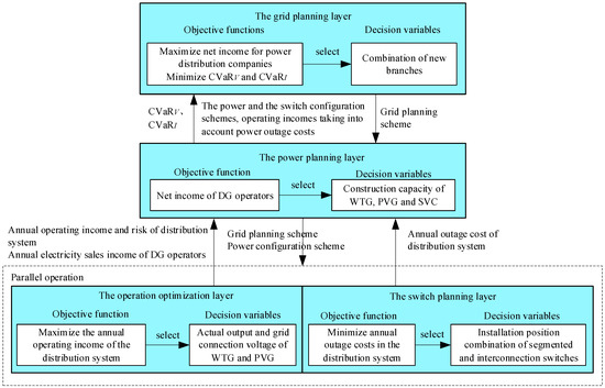
Figure 1.
Model framework for source-grid collaborative planning of distribution system.
2.1. Grid Planning Layer
In order to coordinate the benefits and risks in the distribution grid planning, the grid planning layer aims to maximize the net income F1 of the power distribution company, minimize the conditional value at risk of the node voltage CVaRV and minimize conditional value at risk of the branch current CVaRI. The calculation methods of each goal are as follows:
- Economic income objective F1
To meet the load demand for the next 10 years, a series of grid planning schemes are generated through measures such as building new feeders, renovating, and expanding existing feeders. The expression for the net income F1 of the power distribution company is
where Cnet is the annual grid construction cost. Ctrans, Cgrid, Closs, and CENS are the annual transaction income of the power distribution company, the annual electricity purchase cost from the superior power grid, the annual grid loss cost, and the annual power outage loss cost taking into account the investment cost of switches and connecting feeders.
The expressions for each expense in Formula (1) are
where Γn is the collection of newly built and renovated branches, Lk is the length of the kth branch, Cj,k is the unit length construction cost of the kth branch, depending on the feeder type, cd,k, cu,k are the demolition costs and residual values of the kth branch road, which are not zero only when the branch is renovated. The residual value refers to the value of components that can continue to be used, such as poles and towers. e is the bank rate, Tk is the service life of the kth branch, usually 40 years for cable lines and 30 years for overhead lines, Ns and Ts are the total number of source-load typical scenarios and the annual duration hours of the sth scenario. Csold,s is the electricity price for the sth scenario. NL, NEV, and NDG are node collections containing loads, EV charging facilities, and DG. PL,s,i, PDG,s,i, and PEV,s,i are the conventional load, actual output of DG, and power of EV charging facility at the ith node of the sth scenario. When PEV,s,i is greater than 0, it indicates charging the EV, and when it is less than 0, it indicates discharging the EV. CEV, cEVf and cDG are the charging price for EV, the discharging price for EV, and desulfurization coal benchmark prices. ΓT is the set of branches after the grid structure planning, Is,k and Ploss,s,k are the current and feeder loss power flowing through the kth branch in the sth scenario, ρk is the unit length resistance of the kth branch, Cf, Cp, and Cg are the prices during peak to valley periods, λ1 and λ2 are the threshold for dividing peak and valley periods, and the paper takes 0.7 and 0.8. PL,s, PDG,s, PLD,s, Ploss,s, and PEV,s represent the total conventional load, total DG output, total all loads, grid loss power, and total EV load in the sth scenario. cgrid is the price purchased by the power distribution company from the superior power grid, ENS is the system power shortage in the sth scenario, ΓK and ΓKF refer to the collection of branches for newly built switches and newly built connecting feeders, NK, cK, and TK are the total number of newly added switches, switch cost, and service life.
- 2.
- Conditional value-at-risk objective CVaRV, CVaRI
In order to reduce the risk of node voltage or branch current exceeding the limit caused by the randomness of load prediction error, current research mostly uses opportunity constraints to replace the rigid constraints of node voltage and branch current [19]. The formula is expressed as
where Vs,i is the voltage amplitude of the ith node in the sth scenario, Vmin and Vmax are the upper and lower limits of the node voltage, Ik,max are the maximum operating current of the kth branch, α1 and α2 are the confidence level of node voltage constraints and branch current constraints, and p is the probability of meeting the constraint conditions.
To reduce the difficulty of solving Formula (8), the following assumptions are made:
- (1)
- Prediction error of annual maximum load ΔPL follows normal distribution. ΔPL,i~N(0, ) is the probability distribution of load prediction error for the ith node.
- (2)
- The probability of load prediction error at each node remains equal; for example, the ith and the jth nodes take values separately; ΔP1 and ΔP2 require p(ΔPL,i ≤ ΔP1) equal to p(ΔPL,j ≤ ΔP2).
On the basis of the above assumptions, since the load of any node in the planning model depends on the typical daily load curve of the node and the expected annual maximum load of the node (as shown in Figure A1 of Appendix A), the node voltage and branch current of all scenarios in Formula (8) also obey the normal distribution, and Formula (8) can be simplified as
where ΔPL,i,α indicates that there is a α probability that the load prediction error is greater than ΔPL,i,α, and ΔPL,i,α is called the quantile. Vs,j(ΔPL,i,α) and Is,k(ΔPL,i,α) are the voltage at the jth node and the current flowing through the kth branch when the load of the ith node is taken as PL,s,i + ΔPL,i,α and PL,s,I + ΔPL,i,α.
Due to the fact that the effectiveness of opportunity constraints depends on the value of confidence and the lack of consideration for planning risk levels outside the confidence interval, when the true value of future loads is outside the confidence interval, the node voltage and branch current may seriously exceed the limit. In order to avoid serious consequences caused by small probability events, while satisfying Formula (9), value at risk (VaR) and conditional value at risk (CVaR) theories are introduced.
VaR is a widely used risk measurement method in the financial field. VaR refers to the maximum possible loss of a securities portfolio in the future under a given confidence level [20], and its formula is expressed as
where ΔP is the potential loss of the securities portfolio in the future. VaRα is the value at risk with a confidence level of α, which also indicates that the probability of a portfolio loss greater than VaRα is 1 − α.
Compared to VaR, CVaR highlights the potential risks of investment portfolios and is considered by academia as a more reasonable and effective risk measurement method. CVaR refers to the average loss of a securities portfolio exceeding VaR over a period of time in the future, and its formula is expressed as
where f(x,y) is the loss function, x is the decision variable, and y is the random variable representing the uncertainty factor.
Based on the application scenario of the paper, CVaR refers to when ΔPL exceeds ΔPL,i,α, the time when the node voltage exceeds the limit or the average amplitude of the branch current exceeds the limit is recorded as CVaRV and CVaRI. CVaRV and CVaRI represent the average risk level outside the load confidence interval, and the formula is expressed as
where p(s) is the probability of the sth scenario, nd is the number of nodes in the distribution system, vs,i is whether the voltage of the ith node exceeds the limit.
To reduce the difficulty of solving, the integrals of Formulas (10) and (11) are discretized based on blind numbers. Specifically, the interval [α, 1] is divided into u segments equally, and the mean of each segment is used as the sampling blind number. The sampling blind number is estimated through uniform sampling of the interval, and the integration of the entire interval is replaced by the sum of a finite number of sampling blind numbers [21]. Therefore, the calculation formulas for CVaR and the sampling blind number are
where ΔPL,i,l, ΔPL,i,x are the lth sampling blind number and the xth sampling point of the blind number. p(ΔPL,i,x) is the probability of the xth sampling point. Since the load prediction error is assumed to meet the normal distribution, the probability of sampling points is obtained by transforming the normal distribution into the standard normal distribution and querying the standard normal distribution probability table. nl is the number of samples in the lth interval.
- 3.
- Weighted summation of the objective
To solve the multi-objective problem involving incomes and risks, a linear weighting method based on the subjective and objective weighting is used to transform it into a single objective problem. This method reflects the risk preference of decision-makers through the weight of objectives and comprehensively considers the satisfaction level between multiple objectives with different properties and contradictions, resulting in a balanced improvement of each objective of the plan. The formula is expressed as
where w1 to w3 are the target weights, F1,max, CVaRV,max and CVaRI,max are the maximum values achieved by each target in the decision variable space, F1,min, CVaRV,min and CVaRI,min are the minimum values achieved by each target.
The calculation process of weight is as follows: we assum g decision-makers evaluate the importance of the target and form a decision matrix w = (wij)g×3, where wij is the evaluation value of the ith decision-maker on the jth objective. Based on the opinions of various decision-makers, the expression for the non-normalized objective weight wj is
where βi is the comprehensive weight of the ith decision-maker, δi and ξi are the subjective and the objective weights. Subjective weight δi is determined through mutual evaluation among decision-makers. Objective weight ξi represents the degree of difference between oneself and other decision-makers in target weight decision-making; the smaller the difference, the larger the ξi. ε is a subjective weight preference with a value of [0, 1].
According to Formula (14) and after normalization, the weights of each target are [w1, w2, w3] = [0.5, 0.19, 0.31].
The constraints of the grid planning layer are as follows:
- (1)
- Radiation grid operation constraints. The necessary and sufficient conditions to ensure the open loop operation, grid connectivity and access of all users to the grid in the medium voltage distribution system arewhere npath,i is the number of paths from the beginning of the line to the ith node.
- (2)
- Constraint of outgoing line spacing. Substation nodes without remaining intervals cannot have new feeders.
2.2. Power Planning Layer
The power planning layer aims to maximize the net income of DG operators F2, including (1) the investment cost and equipment operation and maintenance cost of WTG, PVG, and SVC; (2) electricity sales income taking into account policy subsidies. The formula is expressed as
where H is the set of DG types. ch, Th and Pi, h are the unit capacity cost, the service life, and the construction capacity of the hth type of DG at the ith node. cw,h and cbu,h are the maintenance cost and the policy subsidy for the unit power generation of the hth type of DG. Ph,max is the upper limit value of the construction capacity of the hth type of DG considering spatial constraints. SC,i, cC and TC are the newly added capacity, the unit capacity cost, and the service life of SVC at the ith node. SC,i and SC,max are the upper limits of the newly added and the constructed capacity of SVC at the ith node.
2.3. Switch Planning Layer
A strong grid structure and the reasonably distributed switch are two main measures to improve the reliability of the distribution system. The switch planning layer aims to minimize the annual outage cost taking into account social and economic losses. Based on the power and grid planning scheme, the configuration scheme of segmented switches and tie switches is optimized. The formula is expressed as
where cp is the economic benefit created by the unit electricity consumption in the planned area, SAIDI and SAIDI0 are the average power outage time and its upper limit values of the distribution system users. SAIDI and ENS are both obtained through the reliability evaluation method in literature [22].
2.4. Operation Optimization Layer
The operation optimization layer aims to maximize the economic benefits of the power distribution company, takes the actual output of DG and the voltage of the grid connection node as decision variables, and takes power flow constraints of the grid, opportunity constraints of the branch current and the node voltage and output constraints of DG and SVC as constraint conditions. The formula is expressed as follows:
where Ps,i and Qs,i are the active and reactive injection power of the ith node in the sth scenario, j ∈ i is the node directly connected to the ith node (including j = i), Gij and Bij are the real and imaginary parts of the node admittance matrix elements, θij is the voltage phase difference between the ith and the jth nodes, PDG,s,i,max is the theoretical output of DG in the sth scenario, QC,i is the output of SVC at the ith node in sth scenario.
In order to consider the impact of demand response on the operating income of the power grid, the operation optimization layer constructed a user response price model based on the demand price elasticity matrix, focusing on the study of transferable loads and reducible loads. Transferable loads refer to the ability to transfer a peak load to other periods of time, such as partial loads of industrial and commercial users, while the total electricity consumption remains unchanged within a cycle. Reduced loads refer to the ability to reduce electricity consumption during high electricity prices, such as residential air conditioning loads. The response price models for these two types of flexible loads are
where Px,t,0 and Px,t are the reducible loads before and after the response to the price in the tth period. γt is the self-elasticity coefficient of the tth period, csold,0 is the initial price, Psh,t1,0 and ΔPsh,t1 are the transferable load before responding to the price of the t1th period and the amount of transferable load after responding to the price of the t1th period, Γt1 and γt2 are the cross-elasticity coefficients for the t1th and the t2th periods.
To consider the impact of the charging and discharging strategies of EV on the operating income of the power grid, the operational optimization layer studied the load characteristic curves of household EV using two types of strategies: orderly charging and the vehicle-to-grid (V2G) technology. According to the results of the household car survey in the United States, the daily mileage R of the household EV and the end time te of the last trip approximately follow the log-normal distribution and normal distribution [23], and the probability density is, respectively,
where μR = 3.20, σR = 0.88, μt = 17.6, σt = 3.4.
To ensure the normal daily travel of electric vehicles, the state of charge of electric vehicle batteries meets the following constraints:
where SOCt and SOCmin are the state of charge and lower limit values of the battery at time t, ηc and ηf are the charging and the discharging efficiency of the battery, Pc and Pf refer to the charging and discharging power of EV charging facilities, PEV,e is the nameplate capacity of EV battery, Δt is the time step, SOC0 and SOCT are the initial and ending states of charge. Rmax is the maximum distance traveled by EV.
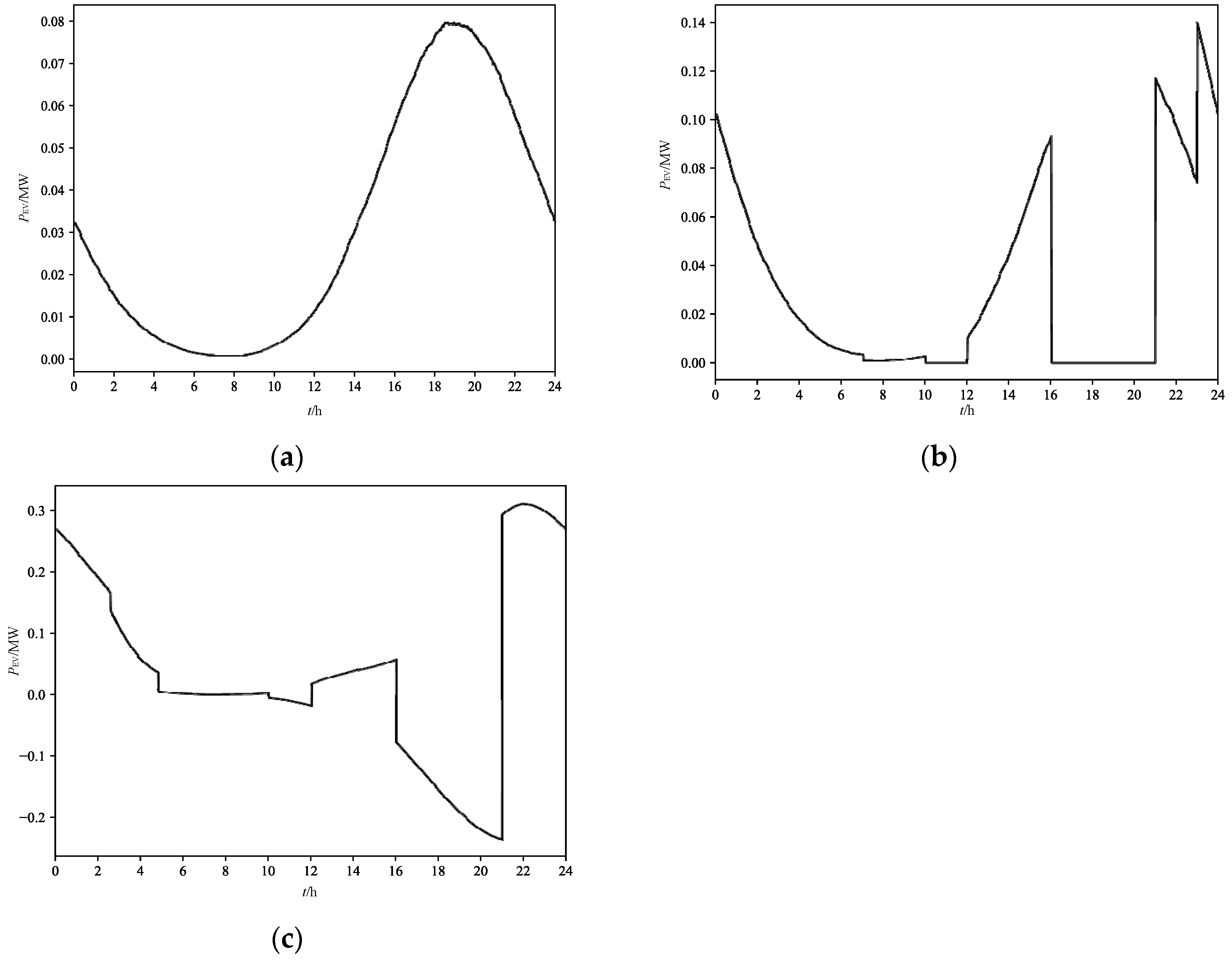
When EVs adopt an orderly charging strategy, the EV load can be considered as a transferable load. We assuming that before responding to the price, te is taken as the starting time tcs of charging. The number of simulation days is 1000. Based on the Monte Carlo method, the charging load curves of 100 household EVs with a battery capacity of 35 kWh and a maximum mileage of 175 km before and after responding to the price are shown in Figure A3a,b of Appendix B.
When EV adopt the V2G mode charging and discharging strategy, the following rules are designed: when the price is at peak hours, EVs are discharged, and the discharge ends when the lower limit of EV battery state of charge is reached. When the price is during the flat or the valley periods, EVs are charged, and the charging ends when the state of charge of the EV battery reaches the upper limit or when the charging reaches 7 o’clock the next day. Taking 100 household EVs as an example, the load characteristic curve of EV based on Monte Carlo method is shown in Figure A3c of Appendix B.
3. Solution of a Multi-Layer Planning Model
3.1. Solution of Grid Planning Layer
Because the distribution grid is a radial topological structure and has connectivity requirements, it can be represented as a tree in graph theory and stored by an adjacency matrix, so this work uses the tree structure coded parthenogenetic algorithm (PGA) to solve the network planning layer. In this work, adjacency matrix is used as genetic coding, which can not only avoid the problem of generating a large number of infeasible solutions and compressing the optimization space in the solution process, but also save decoding work [24]. Considering that PGA with tree structure encoding mainly changes the parent node of a certain node or certain nodes, using selection, shift, and reassignment operators, the selection operator adopts a roulette wheel operation similar to a traditional genetic algorithm while incorporating an optimal individual preservation strategy. Shifting the operator changes the tree structure by randomly selecting a node and changing its parent node. Reassignment operator changes the tree structure by selecting some nodes and changing their parent nodes [25]. The analysis in reference [26] shows that the single parent genetic algorithm encoded by the tree structure mentioned above has global convergence.
3.2. Solution of Power Planning Layer and Operation Optimization Layer
The decision variables of the power planning layer and the operation optimization layer are both continuous variables. For example, the planning content of the power planning layer is the location and capacity determination of WTG, PVG and SVC, and the decision variables are represented as a combination of power capacity of a series of optional nodes. When the power capacity of an optional node is zero, the decision variable represents that no power is configured at that node, so the decision variable of the power planning layer represents the location and capacity information of WTG, PVG and SVC. Similarly, the decision variables of the operational optimization layer are represented as a combination of the voltage and DG output of a series of power nodes.
Because the values of power capacity and node voltage are continuous and have a wide range of values, it is more suitable to use decimal-coded group behavior algorithms to optimize power capacity and node voltage than evolutionary algorithms such as a binary-coded genetic algorithm. Based on various test functions, the experimental results in literature [27] prove that the stability and convergence accuracy of a sparrow search algorithm (SSA) are far better than other group behavior algorithms, such as the bat algorithm and the gray wolf optimization algorithm, so we chose SSA as the solution algorithm for the power planning layer and the operation optimization layer.
3.3. Solution of Switch Planning Layer
To reduce the difficulty of solving the switch planning layer, the following assumptions are made: (1) All switches are automatic circuit breakers; (2) A maximum of one switch can be configured for any branch, which simplifies the optimization configuration problem of switches to an optimization combination problem about whether the branch has switches. Based on the above assumption, the decision variables of the switch planning layer are represented as a combination of state values of a series of branches. If a branch is equipped with an automation switch, the status value of the branch is one; otherwise, the status value of the branch is zero. Because binary-coded genetic algorithms are suitable for optimizing two state decision variables, we chose adaptive genetic algorithm (AGA) as the solution algorithm for the switch programming layer [28].
3.4. Overall Solution Process
Combining Section 3.1, Section 3.2 and Section 3.3 the solution process of the multi-layer programming model is described as follows:
Step 1: Initialize the population X = {x1, …, xNx}, where x represents the new combination of branches to be planned, fx represents the fitness of x, which is equal to the objective function value of the grid planning layer.
Step 2: For each grid scheme x, initialize the population Y = {y1, …, yNy}, where y represents the combined capacity of WTG, PVG, and SVG, and fy represents the fitness of y, which is equal to the objective function value of the power planning layer.
Step 3: For the determined grid scheme x and power supply combination y, initialize the population Z = {z1, …, zNz}, where z represents the actual output of WTG and PVG and their grid connection voltage, and fz represents the fitness of z, which is equal to the objective function value of the operation optimization layer. After obtaining fz based on power flow calculation, determine whether the iteration termination condition has been met. If it is true, terminate the algorithm. Otherwise, update the value of z and continue calculating fz.
The process is similar to the previous steps when initializing the population M = {m1, …, mNm}, where m represents the combination of branch switches or tie switches, and fm represents the fitness of m, which is equal to the objective function value of the switch planning layer. After obtaining fm based on the reliability evaluation algorithm, determine whether the iteration termination condition has been met. If it is true, terminate the algorithm. Otherwise, update the value of m and continue calculating fm.
Step 4: After calculating fy based on the feedback results of the running optimization layer, determine whether the iteration termination condition has been met. If the algorithm is terminated, update the value of y and return to step 3.
Step 5: After calculating fx based on the feedback results of the lower-level model, determine whether the iteration termination condition has been met. If it is true, output the planning results and end algorithm, otherwise update the value of x and return to step 2.
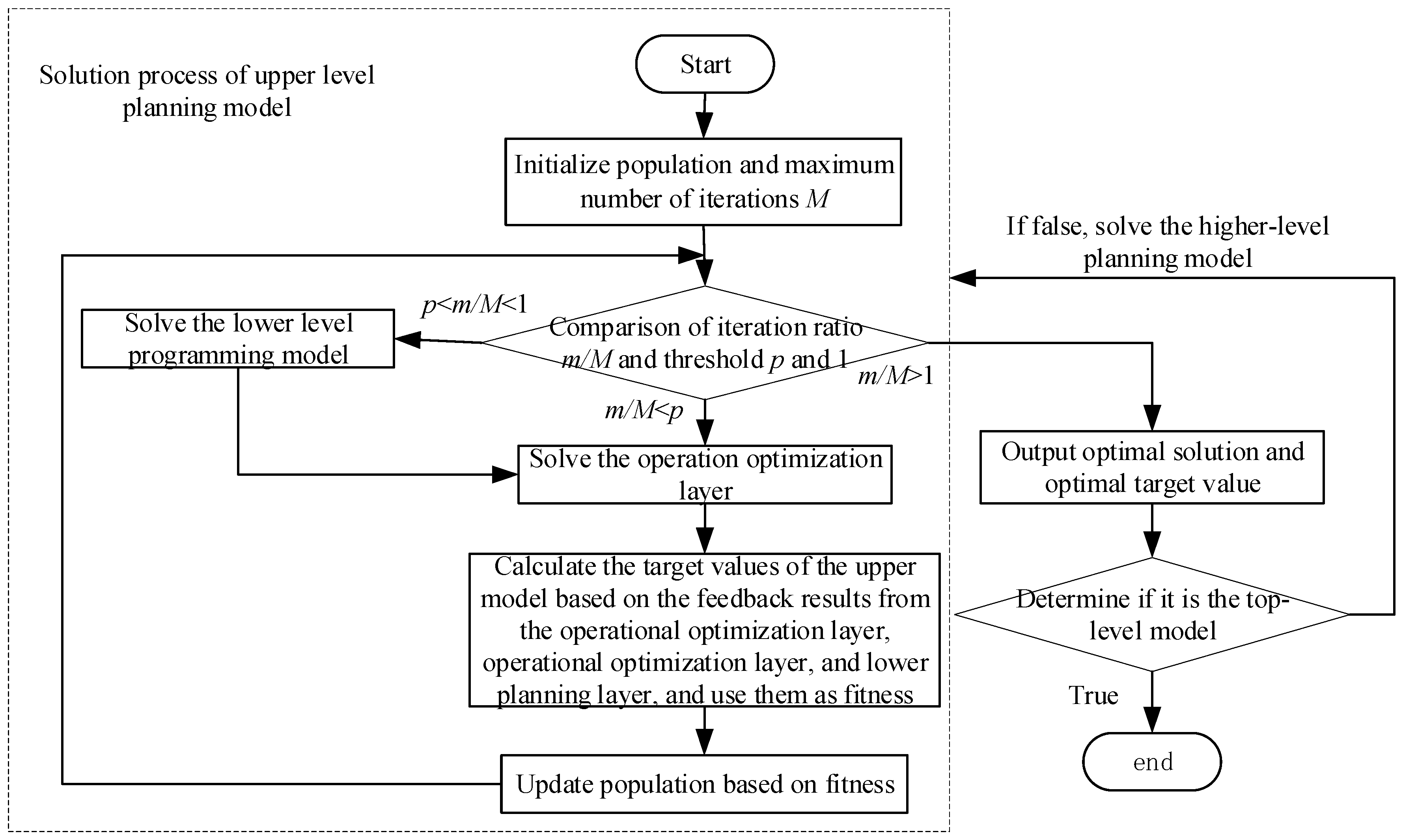
In the process of solving a multi-layer programming model, since calculating the target values of the upper-level model requires feedback from the lower-level model, assuming that the heuristic algorithm for solving each level model has 50 iterations, the number of calls to run the optimization layer is 50 × 50 = 2500 times, which significantly increases the solving time of the multi-layer model as the number of layers increases. Considering that the decision variables of each layer model are the main factors affecting the target value of this layer, for example, the quality of the grid planning scheme is the biggest influencing factor that determines the net benefit of the power distribution company, it is proposed to ignore the influence of the decision variables of the lower level planning model in the early stage of solving the planning model based on heuristic algorithms. In the later stage of optimization, for the first n planning schemes with the optimal target values, the solution strategy for the target values is modified based on the feedback results of the lower level planning model. The strategy proposed in this chapter reduces the number of calls to the lower-level model and shortens the solution time while ensuring the accuracy of the solution. The improved solution process is shown in Figure 2.

Figure 2.
The solution process of multilevel programming model.
With the increase in the number of nodes in the distribution system, the number of dimensions of decision variables in each layer of the multi-layer programming model also increases, which significantly increases the difficulty of solving the model. To reduce the difficulty of solving the model, we propose a partition planning method when the number of nodes in the distribution system exceeds 100, and the process is as follows:
- (1)
- Use the power supply range of each substation as a sub area. Divide the newly added nodes into sub areas corresponding to the nearest substation based on the path distance between the nodes and each substation.
- (2)
- Build multi-layer planning models for each sub region separately, and obtain planning solutions for each sub region based on the solving algorithm proposed in this section.
Because the number of nodes in the sub region is much less than the number of nodes in the distribution system before the partition, the proposed method can effectively reduce the difficulty of solving large-scale distribution systems.
4. Example Analysis
4.1. Basic Data of the Example
The paper selects a 54-node system as an example, and the initial grid structure is shown in Figure A4 of Appendix C. The solid line in Figure A4 represents the branch that has been put into operation, and the dashed line represents the corridor that can be connected. The circles and numbers in Figure A4 represent nodes and their numbers, respectively. The load data of each node and the branch length in Figure A4 are shown, respectively, in Tables S1 and S2 of Supplementary Materials. Assuming there are three optional feeder types, their specific parameters are shown in Table A1 of Appendix D.
Assuming the power factors of industrial, commercial, and residential loads are 0.8, 0.85, and 0.9, and their typical daily power curves for the four seasons are shown in Figure A1. Assuming that all industrial loads participate in demand response and are considered transferable loads, 50% of commercial and residential loads participate in demand response and are considered reducible loads. We assume that the self-elasticity coefficient of the reducible load at each period is −0.1, and the flat-valley cross elasticity coefficient, peak-valley cross-elasticity coefficient, and peak-flat cross-elasticity coefficient of transferable loads are 0.012, 0.016, and 0.01.
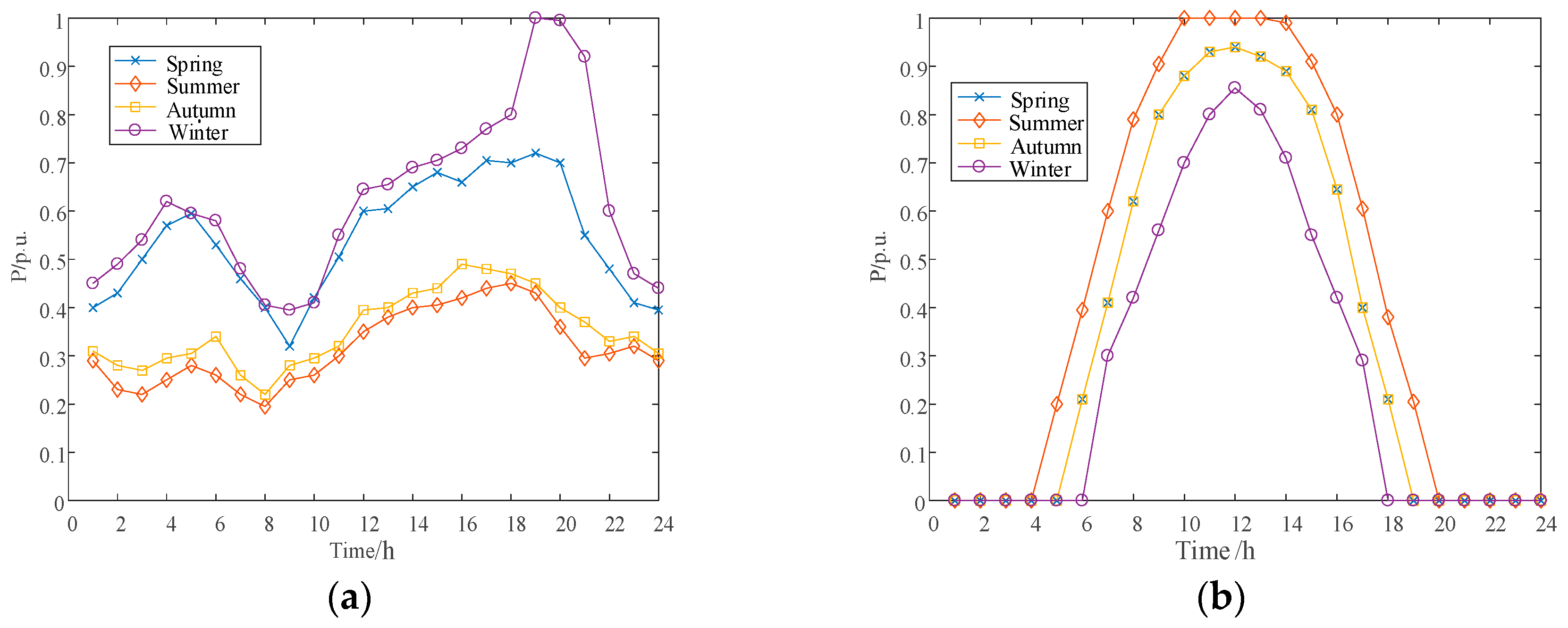
Assuming that the maximum access capacities of WTG, PVG, and SVC at a single node are 2, 1.5, and 1 MW, the power parameters are shown in Table A2 of Appendix D, and the typical daily output curves of WTG and PVG for four seasons are shown in Figure A2 of Appendix A.
The electricity prices related to the income of the power distribution company are shown in Table A3 of Appendix D. We assume the original electricity price before implementing the time of use electricity price is 0.6 yuan/kWh.
4.2. Revenue Analysis of the Source and Grid under Different Planning Methods
The paper uses different planning methods to solve the grid planning problem in Appendix C and obtains the following planning schemes:
Scheme 1: Adopting the method proposed in this paper.
Scheme 2: Without considering planning risks, the grid planning layer takes the net income of the power distribution company as a single goal.
Scheme 3: Regardless of the differences in stakeholders between the source and the grid, the planning model aims to minimize the annual comprehensive cost of the grid including DG investment and construction costs.
Scheme 4: Without considering power planning, the planning model aims to minimize the annual comprehensive cost of the grid.
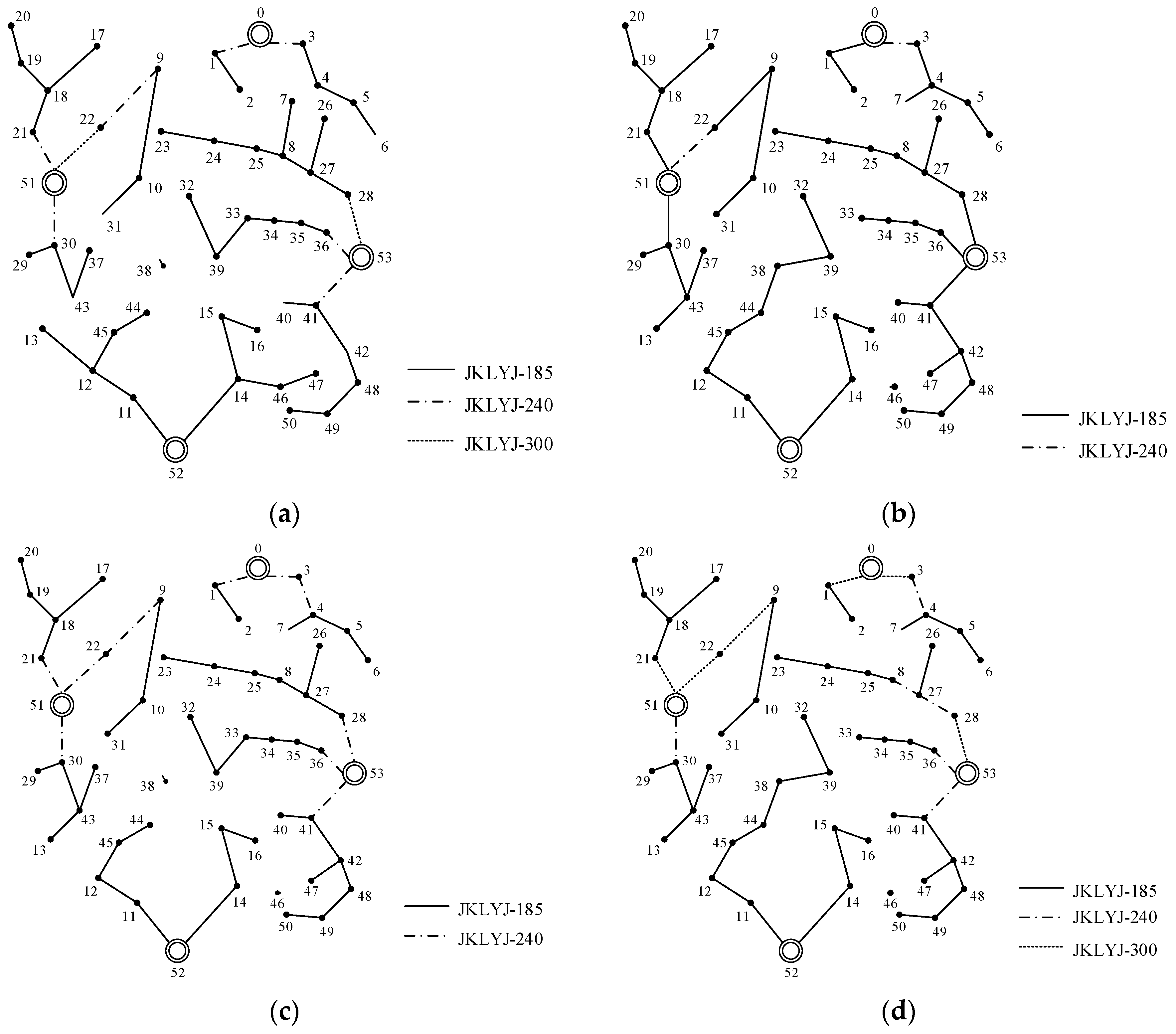
The grid planning results of each scheme are shown in Figure 3, with the main differences reflected in the grid structure and the feeder type, which affect the construction cost and annual grid loss. The power planning results of each scheme are shown in Table A4 of Appendix D, and the switch planning results of Scheme 1 are shown in Table A5 of Appendix D. See Table 1 and Table 2 for the cost details of the power distribution company and the DG operators, respectively. The total net income is shown in Figure 4, and Table 3 describes the conditional value at risk of node voltage and branch current. By comparing and analyzing the index of each scheme in Table 1, Table 2 and Table 3, it can be concluded that:

Figure 3.
Grid planning results in each planning scheme. (a) Scheme 1; (b) Scheme 2; (c) Scheme 3.; (d) Scheme 4.

Table 1.
Various costs of the power distribution company in each planning scheme.
Table 2.
Various costs of the DG operators in each planning scheme.

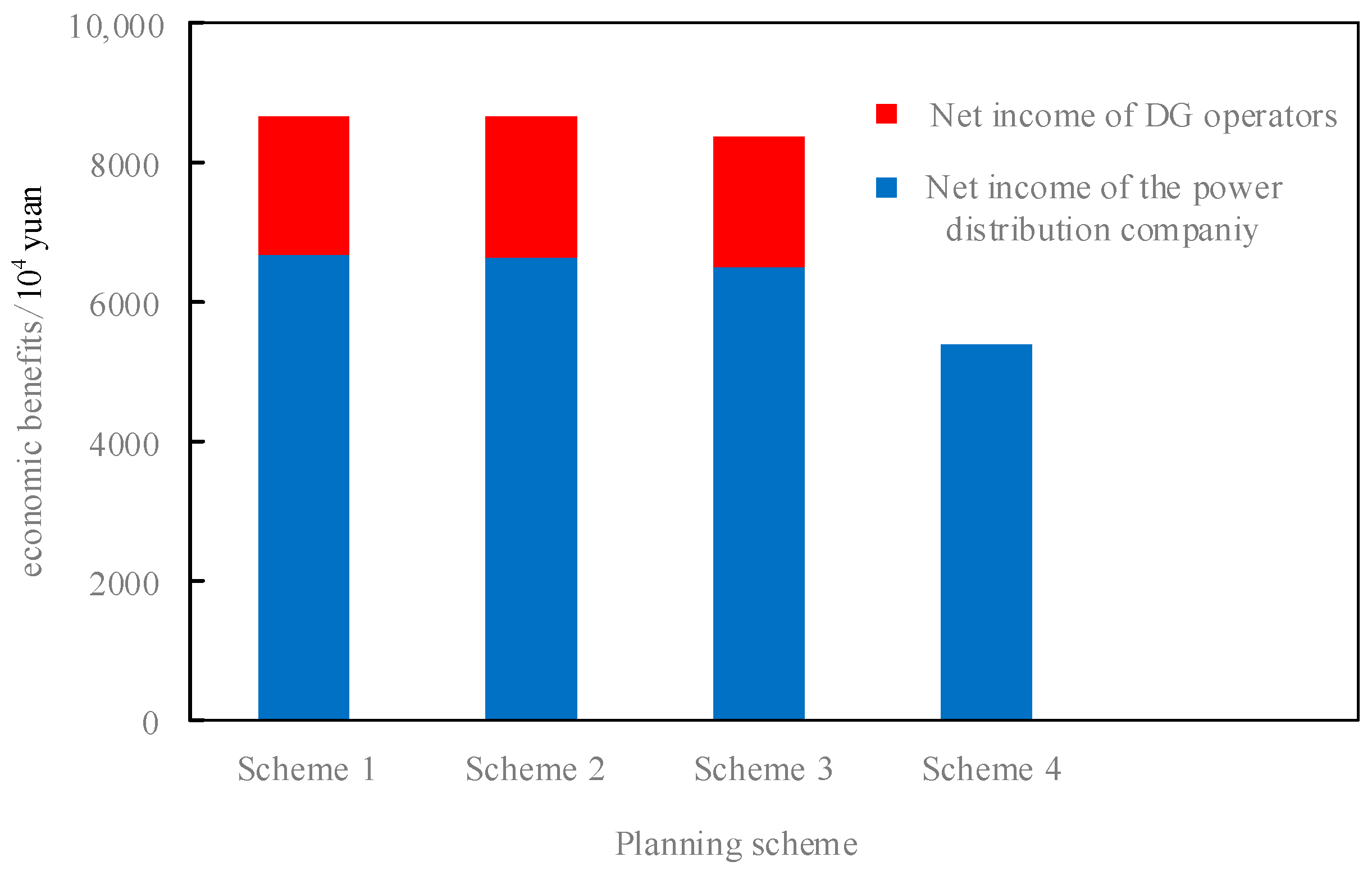
Figure 4.
The sum of the net income of both parties in each planning scheme.
Table 3.
Multiple planning risks in each planning scheme.
- (1)
- Scheme 1 has the lowest risk of branch current exceeding the limit, which means that the proposed method significantly reduces the planning risk caused by load uncertainty.
- (2)
- Compared to Scheme 2, Scheme 1 has a higher construction cost for the grid structure, because under opportunity constraints, the grid structure needs to meet larger grid supply load scenarios than the expected value of load forecasting, resulting in some branches choosing feeder types with larger current limit values.Compared to Scheme 2, DG operators have lower net profits and higher power investment costs in Scheme 1. This is because the planning model aimed at planning risks tends to increase DG investment capacity, resulting in an increase in DG theoretical output. By supplying power to surrounding loads through DG, the feeder load and the risk of branch current exceeding the limit is reduced. However, due to the fact that the electricity sales revenue of the DG operators is mainly determined by the expected annual maximum load, the increase in electricity sales revenue is smaller than the increase in cost, resulting in a decrease in the net benefit of the DG operators in Scheme 1.
- (3)
- Compared to the income type planning models, namely Scheme 1 and Scheme 2, the net income of the power distribution company and the DG operators in Scheme 3 is lower. This is because Scheme 3 is based on the cost type planning model, and the objective function does not include the increase in sales income of the DG operators, which leads to a faster decrease in marginal benefits of investing in DG and a conservative trend in power investment. The decrease in DG investment capacity leads to a decrease in both the actual output of DG and the sales income of the DG operators. At the same time, the risk of branch current exceeding the limit and the cost of purchasing electricity for the power distribution company increase with the increase in grid supply load. In summary, the power planning obtained based on the cost type planning model is conservative, causing the economic benefits of both the source and the grid to deviate from the optimal. Therefore, the income type planning model is more reasonable than the cost type planning model.
- (4)
- In Scheme 4, the net income of the power distribution company is the lowest, the grid construction cost is the highest, and the annual grid loss is more than 50% higher than other schemes. This is because Scheme 4 is based on traditional network planning methods, which makes it impossible for the power distribution company to reduce the purchase cost by purchasing electricity from DG operators or reducing feeder load by consuming DG nearby. Comparing the total net benefits of the source and the grid in each scheme in Figure 4, it can be seen that compared to the traditional grid planning method, which is Scheme 4, the collaborative planning method for the source and the grid, which is Scheme 1 to Scheme 3, creates higher economic value. In addition, combined with Figure 3d and Table 3, it can be seen that in Scheme 4, although more current limiting feeder types are selected for multiple branches, the conditional value at risk of the node voltage and the branch current is still higher than that of other schemes, which again proves that DG power supply can effectively reduce the adverse impact of load uncertainty on the distribution system.
4.3. Revenue Analysis of the Source and the Grid under Different Operating Strategies
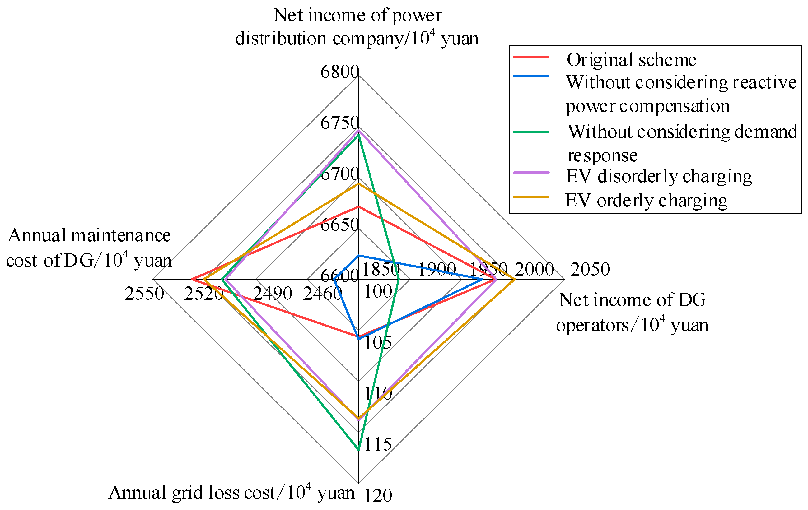
In the operation optimization layer constructed in this paper, a 10 kV reactive power compensation, demand response of electricity price type and orderly charging and discharging of EVs are considered. To quantify the impact of the above operational strategies on the distribution system, based on Scheme 1, various cost changes for the power distribution company and the DG operators were studied separately under different circumstances, such as not considering reactive power compensation, as shown in Figure 5. From Figure 5, it can be seen that:
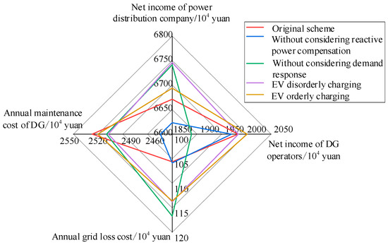
Figure 5.
Cost changes for both parties in each planning scheme under different operating strategies.
- (1)
- Without considering reactive power compensation, the economic benefits of both power distribution company and DG operators decrease. This is because when DG supplies power to the load near the head of the feeder and the reactive power compensation of the gird is insufficient, in order to prevent the voltage of the DG connection point from exceeding the upper limit, the actual output of the DG decreases.
- (2)
- After not considering demand response, the annual grid loss and the net profit of the power distribution company both increase. This is because without considering demand response, the peak valley difference of the load and the annual electricity consumption increase, resulting in an increase in the maximum load current and annual electricity sales of the feeder.
- (3)
- Comparing different charging and discharging strategies of electric vehicles, it can be seen that the annual grid loss and the net profit of the power distribution company achieves the lowest value under the ordered charging and discharging strategy, and the highest value under the disordered charging strategy. This is because under the disordered charging strategy, the overlap between the electric vehicle load curve and the conventional load curve during peak periods is high, further increasing the maximum load current of the feeder. However, under the ordered charging and discharging strategy, the power distribution company purchases electricity from electric vehicle users during peak load periods, reducing the grid supply load through discharging of electric vehicles. Compared with the ordered charging strategy, the load of electric vehicles can be negative under the ordered charging and discharging strategy, and the load adjustment ability is stronger.
- (4)
- According to Formula (16), it can be seen that the maintenance cost of DG is directly proportional to the power generation of DG. Therefore, by comparing the annual maintenance cost of DG under different conditions, it can be concluded that demand response and orderly charging and discharging of electric vehicles contribute to the absorption of the DG output.
5. Conclusions
The paper proposes a multi-factor collaborative planning model which has obtained a planning scheme including grid, DG, reactive power compensation equipment and switches in the next 10 years. In the model, we propose a more comprehensive risk measurement method based on the combination of conditional value at risk theory and opportunity constraint theory. Taking a certain planning area as an example, the effectiveness of the method is verified and the following conclusions are obtained:
- (1)
- Compared with other planning method, the proposed risk measurement method in this paper reduces planning risks caused by load uncertainty by more than 50%.
- (2)
- Compared with the cost-oriented planning model, the proposed multi-factor collaborative planning model in this paper distinguishes the differences in interests of the power distribution company and the DG operators, so that both parties increased the annual net income by 1.5 million yuan and 1.1 million yuan, respectively. Compared with the traditional power distribution grid planning method, the coordinated planning method for the source and the grid effectively reduces the construction cost and the grid loss and improves the economic income of the power distribution company.
- (3)
- Reactive power planning improves the economic benefits of the power distribution company and the DG operators. Although demand response and EV orderly charging and discharging have slightly reduced the net income of the power distribution company, they have the effect of cutting peak load and filling valley load, reducing grid loss, and helping to absorb DG output in flat and valley periods.
In this work, we assume that the probability of load forecasting error of each node on the same feeder remains the same, which is somewhat different from reality. Therefore, the prospect of future research is to further study the estimation method of joint probability distribution of each load on the same feeder when calculating the conditional value at risk.
Supplementary Materials
The following supporting information can be downloaded at: https://www.mdpi.com/article/10.3390/en16155648/s1, Table S1: load data of each node; Table S2: line length of each branch.
Author Contributions
Conceptualization, J.D. and L.L.; methodology, J.D.; software, J.D.; validation, J.D., Y.Z. and Y.M.; formal analysis, J.D.; investigation, L.L.; resources, L.L.; data curation, J.D.; writing—original draft preparation, J.D.; writing—review and editing, Y.Z.; visualization, Y.M.; supervision, J.D.; project administration, L.L.; funding acquisition, L.L. All authors have read and agreed to the published version of the manuscript.
Funding
This research was supported by State Key Laboratory of HVDC(SKLHVDC-2022-KF-01).
Data Availability Statement
The data presented in this study are available in insert article and supplementary material here.
Conflicts of Interest
The authors declare no conflict of interest. The funders had no role in the design of the study; in the collection, analyses, or interpretation of data; in the writing of the manuscript; or in the decision to publish the results.
Appendix A
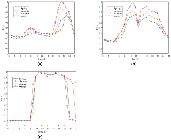
Figure A1.
Four seasons of typical daily power curves of different load types. (a) Resident load; (b) Industrial load; (c) Business load.
Figure A1.
Four seasons of typical daily power curves of different load types. (a) Resident load; (b) Industrial load; (c) Business load.
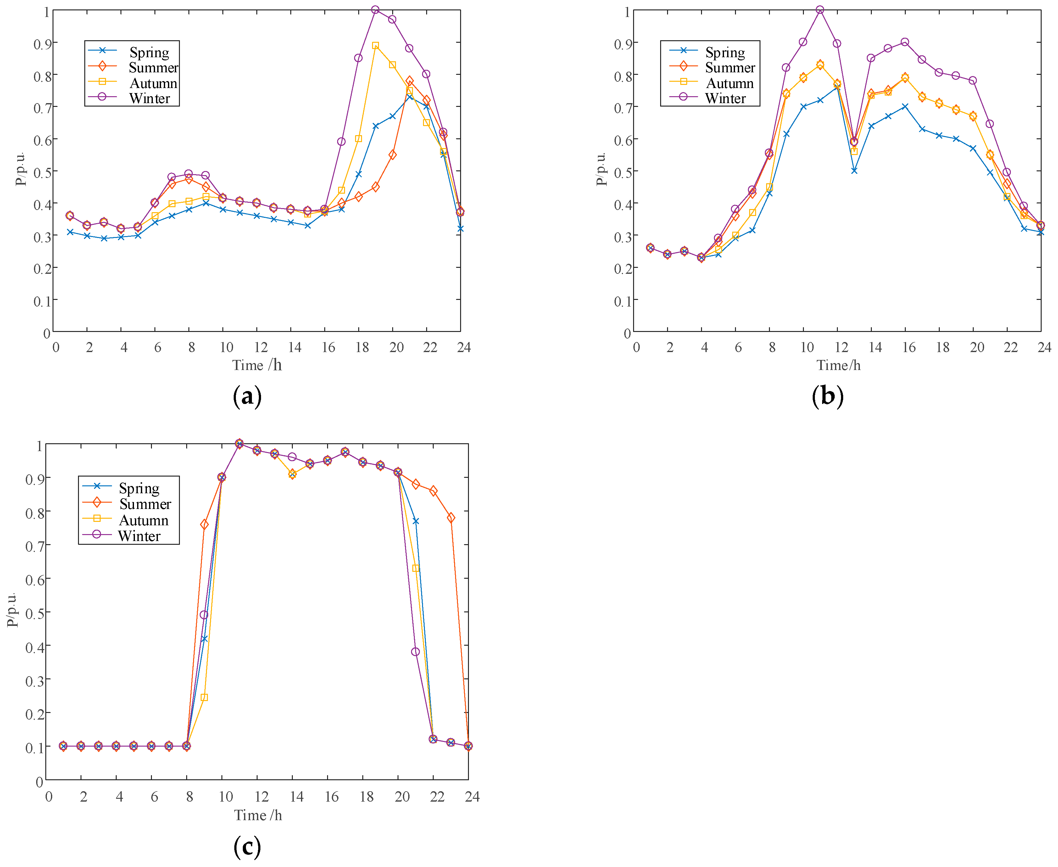
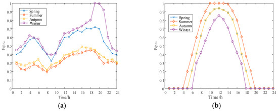
Figure A2.
Four seasons of typical daily output curves of different DG types. (a) Wind turbine generator; (b) photovoltaic generator.
Figure A2.
Four seasons of typical daily output curves of different DG types. (a) Wind turbine generator; (b) photovoltaic generator.
Appendix B
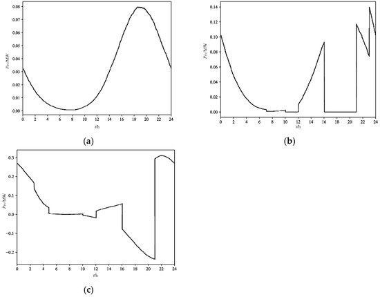
Figure A3.
Load characteristic curve of EV. (a) Disorderly charging; (b) Orderly charging; (c) Orderly charging and discharging.
Figure A3.
Load characteristic curve of EV. (a) Disorderly charging; (b) Orderly charging; (c) Orderly charging and discharging.
Appendix C
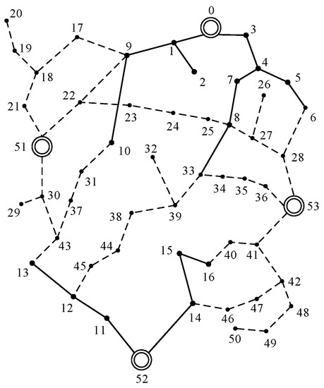
Figure A4.
Area to be planned.
Figure A4.
Area to be planned.

Appendix D
Table A1.
Parameters of selectable feeder types.
Table A1.
Parameters of selectable feeder types.
| Feeder Type | Maximum Allowable Current/A | Cost of Construction/104 Yuan·kWh−1 | Resistance/Ω·km−1 | Reactance/Ω·km−1 |
|---|---|---|---|---|
| JKLYJ-185 | 423 | 24 | 0.164 | 0.308 |
| JKLYJ-240 | 503 | 30 | 0.125 | 0.3 |
| JKLYJ-300 | 583 | 35 | 0.1 | 0.293 |
Table A2.
Parameters of different power types.
Table A2.
Parameters of different power types.
| Power Type | Equipment Life/Year | Cost of Construction/104 Yuan·kWh−1 | Annual Maintenance Cost/Yuan·kWh−1 | Feed-in Tariff/Yuan·kWh−1 |
|---|---|---|---|---|
| WTG | 15 | 230 | 0.3 | 0.6 |
| PVG | 20 | 320 | 0.2 | 0.6 |
| SVC | 10 | 66 | — | — |
Table A3.
Price values related to the power distribution company revenue.
Table A3.
Price values related to the power distribution company revenue.
| Period | Conventional Load Price/Yuan·kWh−1 | Price for EV Charge (Including Service Fee)/Yuan·kWh−1 | Price for EV Discharge/Yuan·kWh−1 | Price for Purchasing Electricity from the Superior Power Grid/Yuan·kWh−1 | Price for Purchasing Electricity from DG Operators/Yuan·kWh−1 |
|---|---|---|---|---|---|
| Peak period | 0.9 | 1.8 | 1.6 | 0.4 | 0.27 |
| Peacetime period | 0.6 | 1.4 | — | ||
| Valley period | 0.3 | 1.2 | — |
Table A4.
Power planning results in each planning scheme.
Table A4.
Power planning results in each planning scheme.
| Planning Scheme | Grid Connection Nodes of WTG (Construction Capacity of WTG/MW) | Grid Connection Nodes of PVG (Construction Capacity of PVG/MW) | Grid Connection Nodes of SVC (Construction Capacity of SVC/MW) |
|---|---|---|---|
| Scheme 1 | 1 (0.45), 5 (2), 8 (0.96), 14 (2), 15 (1.6), 16 (1.7), 22 (1.18), 24 (1.87), 29 (2), 30 (1.94), 33 (1.11) | 1 (0.77), 5 (1.5), 8 (1.24), 14 (1.5), 15 (0.83), 16 (0.93), 19 (1.4), 24 (0.77), 29 (1.5), 30 (0.9), 33 (1.05) | 1 (0.38), 8 (0.37), 14 (0.19), 15 (0.96), 16 (0.48), 19 (0.2), 22 (1), 24 (0.69), 29 (0.34), 30 (0.48), 33 (0.6) |
| Scheme 2 | 1 (0.89), 5 (1.49), 8 (1.44), 14 (1.4), 15 (1.63), 16 (1.38), 19 (1.36), 22 (0.43), 24 (1.3), 29 (1.62), 30 (1.13), 33 (1.65) | 1 (1.28), 5 (1.45), 8 (1.33), 14 (0.16), 15 (0.69), 16 (1.44), 19 (0.53), 22 (0.72), 24 (0.84), 29 (0.42), 30 (1.06), 33 (1.32) | 1 (0.27), 5 (0.64), 8 (0.98), 14 (0.51), 15 (0.97), 16 (0.56), 19 (0.85), 22 (0.31), 29 (0.13), 30 (0.61) |
| Scheme 3 | 1 (0.66), 5 (1.84), 8 (0.35), 14 (0.43), 15 (1.82), 16 (0.46), 19 (2), 22 (1), 24 (0.25), 29 (1), 30 (0.22), 33 (0.26) | 1 (1.12), 5 (1.28), 8 (1.33), 14 (0.94), 15 (0.21), 19 (1.45), 19 (1.4), 24 (1.36), 29 (1), 30 (0.22), 33 (0.26) | — |
| Scheme 4 | — | — | — |
Table A5.
Planning results of the switches and the interconnection feeders in Scheme 1.
Table A5.
Planning results of the switches and the interconnection feeders in Scheme 1.
| Branch with Segmented Switch | Interconnection Feeders | Investment Cost of Switches and Interconnection Feeders/104 Yuan | Annual Power Outage Losses Taking into Account Socio-Economic Losses/104 Yuan |
|---|---|---|---|
| (0, 1), (0, 3), (11, 52), (14, 52), (41, 53), (36, 53), (28, 53), (30, 51), (22, 51), (21, 51), (1, 2), (9, 10), (3, 4), (4, 5), (5, 6), (11, 12), (12, 13), (14, 15), (46, 47), (40, 41), (41, 42), (33, 34), (27, 28), (8, 27), (12, 45), (33, 39), (32, 39), (37, 43), (10, 31), (8, 25), (9, 22), (18, 21), (18, 19) | (1, 9), (9, 17), (4, 7), (38, 44), (38, 39), (31, 37), (42, 47) | 35.86 | 35.4 |
References
- Vahidinasab, V.; Tabarzadi, M.; Arasteh, H.; Alizadeh, M.I.; Beigi, M.M.; Sheikhzadeh, H.R.; Mehran, K.; Sepasian, M.S. Overview of Electric Energy Distribution Networks Expansion Planning. IEEE Access 2020, 8, 34750–34769. [Google Scholar] [CrossRef]
- Cheng, S.; Gu, C.; Yang, X.; Li, S.; Fang, L.; Li, F. Network Pricing for Multi-Energy Systems Under Long-Term Load Growth Uncertainty. IEEE Trans. Smart Grid 2022, 13, 2715–2729. [Google Scholar] [CrossRef]
- Jabr, R.A. Polyhedral Formulations and Loop Elimination Constraints for Distribution Network Expansion Planning. IEEE Trans. Power Syst. 2013, 28, 1888–1897. [Google Scholar] [CrossRef]
- Dehghani, N.L.; Mohammadi-Darestani, Y.; Shafieezadeh, A. Optimal Life-Cycle Resilience Enhancement of Aging Power Distribution Systems: A MINLP-Based Preventive Maintenance Planning. IEEE Access 2020, 8, 22324–22334. [Google Scholar] [CrossRef]
- Wang, M.; Yang, M.; Fang, Z.; Wang, M.; Wu, Q. A Practical Feeder Planning Model for Urban Distribution System. IEEE Trans. Power Syst. 2023, 38, 1297–1308. [Google Scholar] [CrossRef]
- Cuenca, J.J.; Hayes, B.P. Non-Bias Allocation of Export Capacity for Distribution Network Planning with High Distributed Energy Resource Integration. IEEE Trans. Power Syst. 2022, 37, 3026–3035. [Google Scholar] [CrossRef]
- Wankhede, S.K.; Paliwal, P.; Kirar, M.K. Bi-Level Multi-Objective Planning Model of Solar PV-Battery Storage-Based DERs in Smart Grid Distribution System. IEEE Access 2022, 10, 14897–14913. [Google Scholar] [CrossRef]
- Ghamsari-Yazdel, M.; Esmaili, M.; Amjady, N.; Chung, C.Y. Interactive Distribution Expansion and Measurement Planning Considering Controlled Partitioning. IEEE Trans. Smart Grid 2023, 14, 2948–2959. [Google Scholar] [CrossRef]
- Kabirifar, M.; Fotuhi-Firuzabad, M.; Moeini-Aghtaie, M.; Pourghaderi, N.; Shahidehpour, M. Reliability-Based Expansion Planning Studies of Active Distribution Networks with Multi-Agents. IEEE Trans. Smart Grid 2022, 13, 4610–4623. [Google Scholar] [CrossRef]
- Tao, Y.; Qiu, J.; Lai, S.; Sun, X.; Zhao, J. Adaptive Integrated Planning of Electricity Networks and Fast Charging Stations Under Electric Vehicle Diffusion. IEEE Trans. Power Syst. 2022, 38, 499–513. [Google Scholar] [CrossRef]
- Yi, J.H.; Cherkaoui, R.; Paolone, M.; Shchetinin, D.; Knezovic, K. Optimal Co-Planning of ESSs and Line Reinforcement Considering the Dispatchability of Active Distribution Networks. IEEE Trans. Power Syst. 2023, 38, 2485–2499. [Google Scholar] [CrossRef]
- Wolgast, T.; Ferenz, S.; Nieße, A. Reactive Power Markets: A Review. IEEE Access 2022, 10, 28397–28410. [Google Scholar] [CrossRef]
- Jooshaki, M.; Abbaspour, A.; Fotuhi-Firuzabad, M.; Muñoz-Delgado, G.; Contreras, J.; Lehtonen, M.; Arroyo, J.M. An Enhanced MILP Model for Multistage Reliability-Constrained Distribution Network Expansion Planning. IEEE Trans. Power Syst. 2022, 37, 118–131. [Google Scholar] [CrossRef]
- Pamshetti, V.B.; Singh, S.; Thakur, A.K.; Babu, T.S.; Patnaik, N.; Krishna, G.H. Cooperative Operational Planning Model for Distributed Energy Resources with Soft Open Point in Active Distribution Network. IEEE Trans. Ind. Appl. 2023, 59, 2140–2151. [Google Scholar] [CrossRef]
- Li, J.; Xu, Z.; Liu, H.; Wang, C.; Wang, L.; Gu, C. A Wasserstein Distributionally Robust Planning Model for Renewable Sources and Energy Storage Systems Under Multiple Uncertainties. IEEE Trans. Sustain. Energy 2023, 14, 1346–1356. [Google Scholar] [CrossRef]
- Wang, S.; Dong, Y.; Zhao, Q.; Zhang, X. Bi-level Multi-objective Joint Planning of Distribution Networks Considering Uncertainties. J. Mod. Power Syst. Clean Energy 2022, 10, 1599–1613. [Google Scholar] [CrossRef]
- Mejia, M.A.; Macedo, L.H.; Munoz-Delgado, G.; Contreras, J.; Padilha-Feltrin, A. Multistage Planning Model for Active Distribution Systems and Electric Vehicle Charging Stations Considering Voltage-Dependent Load Behavior. IEEE Trans. Smart Grid 2022, 13, 1383–1397. [Google Scholar] [CrossRef]
- Rayati, M.; Bozorg, M.; Cherkaoui, R.; Carpita, M. Distributionally Robust Chance Constrained Optimization for Providing Flexibility in an Active Distribution Network. IEEE Trans. Smart Grid 2022, 13, 2920–2934. [Google Scholar] [CrossRef]
- Bosisio, A.; Berizzi, A.; Amaldi, E.; Bovo, C.; Sun, X.A. Optimal Feeder Routing in Urban Distribution Networks Planning with Layout Constraints and Losses. J. Mod. Power Syst. Clean Energy 2020, 8, 1005–1014. [Google Scholar] [CrossRef]
- Almeida, J.; Soares, J.; Lezama, F.; Vale, Z. Robust Energy Resource Management Incorporating Risk Analysis Using Conditional Value-at-Risk. IEEE Access 2022, 10, 16063–16077. [Google Scholar] [CrossRef]
- Zhang, J.; Wang, Y.; Sun, M.; Zhang, N. Two-Stage Bootstrap Sampling for Probabilistic Load Forecasting. IEEE Trans. Eng. Manag. 2022, 69, 720–728. [Google Scholar] [CrossRef]
- Lin, D.; Liu, Q.; Li, Z.; Zeng, G.; Wang, Z.; Yu, T.; Zhang, J. Elaborate Reliability Evaluation of Cyber Physical Distribution Systems Considering Fault Location, Isolation and Supply Restoration Process. IEEE Access 2020, 8, 128574–128590. [Google Scholar] [CrossRef]
- Hoang, P.H.; Ozkan, G.; Badr, P.R.; Papari, B.; Edrington, C.S.; Zehir, M.A.; Hayes, B.; Mehigan, L.; Al Kez, D.; Foley, A.M. A Dual Distributed Optimal Energy Management Method for Distribution Grids with Electric Vehicles. IEEE Trans. Intell. Transp. Syst. 2022, 23, 13666–13677. [Google Scholar] [CrossRef]
- Vanderstar, G.; Musilek, P. Optimal Design of Distribution Overhead Powerlines Using Genetic Algorithms. IEEE Trans. Power Deliv. 2022, 37, 1803–1812. [Google Scholar] [CrossRef]
- Mahdavi, M.; Alhelou, H.H.; Bagheri, A.; Djokic, S.Z.; Ramos, R.A.V. A Comprehensive Review of Metaheuristic Methods for the Reconfiguration of Electric Power Distribution Systems and Comparison with a Novel Approach Based on Efficient Genetic Algorithm. IEEE Access 2021, 9, 122872–122906. [Google Scholar] [CrossRef]
- Zhou, L.; Sheng, W.; Liu, W.; Ma, Z. An optimal expansion planning of electric distribution network incorporating health index and non-network solutions. CSEE J. Power Energy Syst. 2020, 6, 81–692. [Google Scholar] [CrossRef]
- Yuan, J.; Zhao, Z.; Liu, Y.; He, B.; Wang, L.; Xie, B.; Gao, Y. DMPPT Control of Photovoltaic Microgrid Based on Improved Sparrow Search Algorithm. IEEE Access 2021, 9, 16623–16629. [Google Scholar] [CrossRef]
- Zheng, B.; Li, X.; Tian, Z.; Meng, L. Optimization Method for Distributed Database Query Based on an Adaptive Double Entropy Genetic Algorithm. IEEE Access 2022, 10, 4640–4648. [Google Scholar] [CrossRef]

Disclaimer/Publisher’s Note: The statements, opinions and data contained in all publications are solely those of the individual author(s) and contributor(s) and not of MDPI and/or the editor(s). MDPI and/or the editor(s) disclaim responsibility for any injury to people or property resulting from any ideas, methods, instructions or products referred to in the content. |
© 2023 by the authors. Licensee MDPI, Basel, Switzerland. This article is an open access article distributed under the terms and conditions of the Creative Commons Attribution (CC BY) license (https://creativecommons.org/licenses/by/4.0/).