
A Systemic Comparison of Physical Models for Simulating Surfactant–Polymer Flooding


Abstract
:1. Introduction
2. Materials and Methods
2.1. Modeling Approach
2.2. One-Dimensional Model
2.3. Three-Dimensional Model
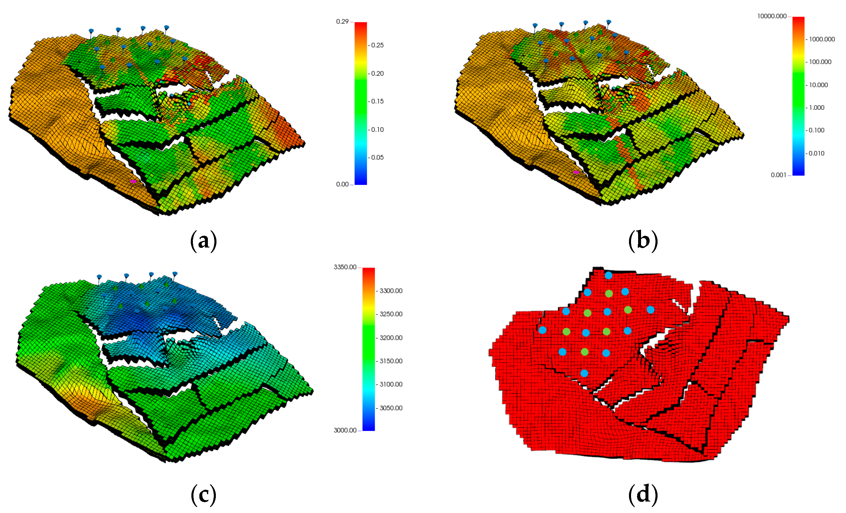
2.4. Field-Scale Model
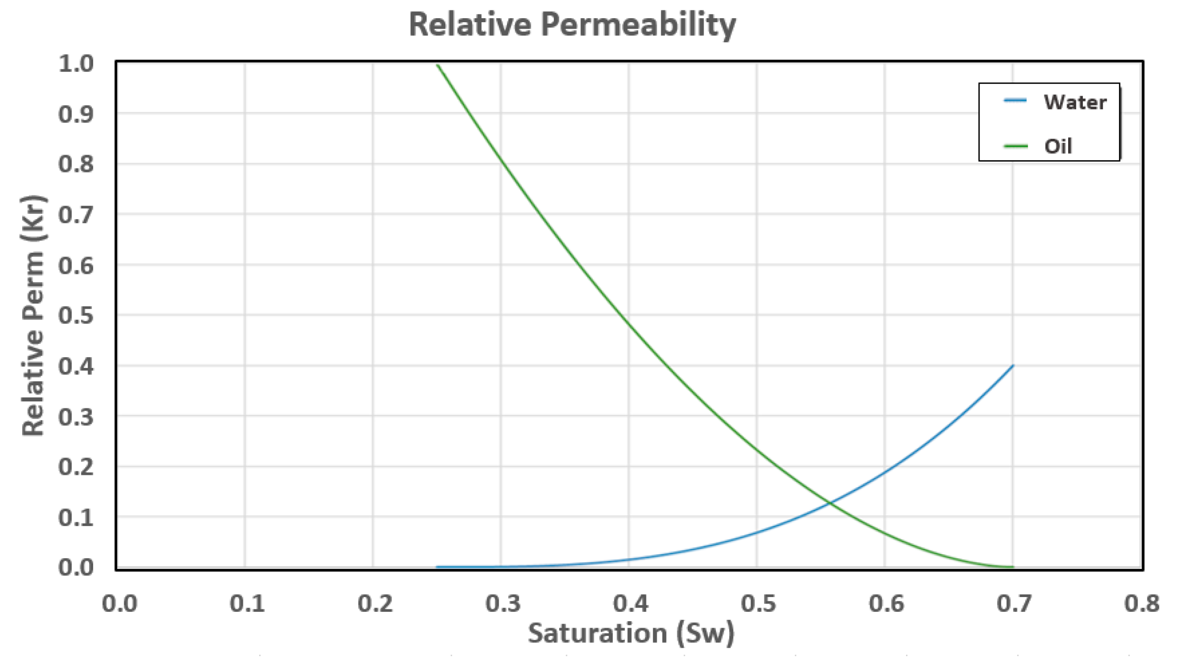
2.5. Summary of Physical Properties
2.6. Waterflood
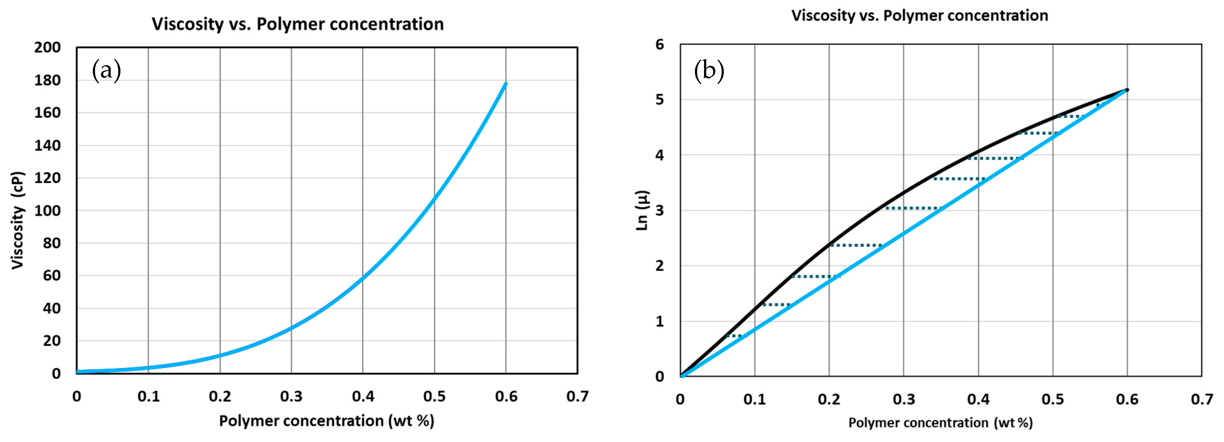
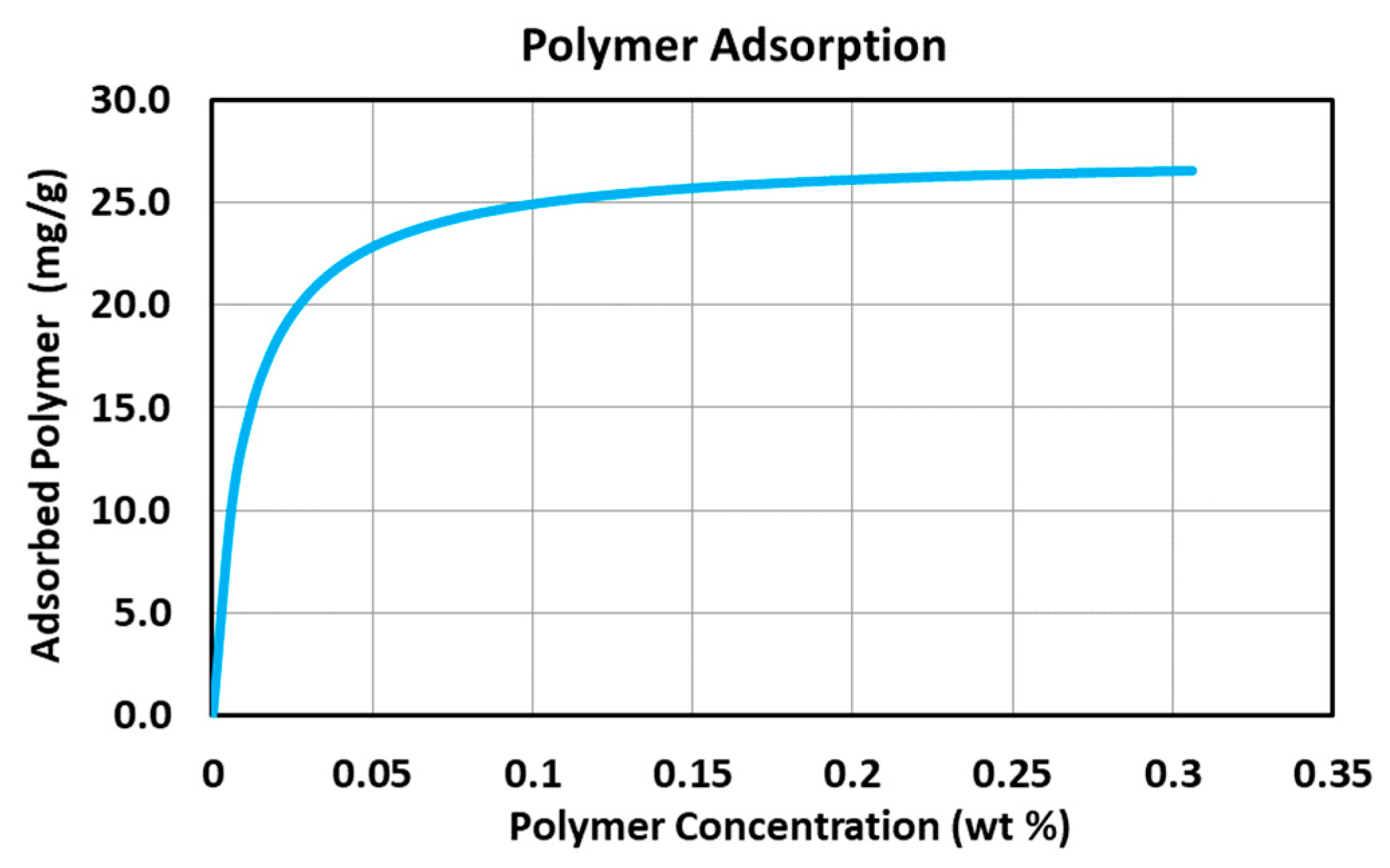
2.7. Polymer Flood
2.8. Surfactant–Polymer Flood
3. Results
3.1. 1D Model Simulation Cases
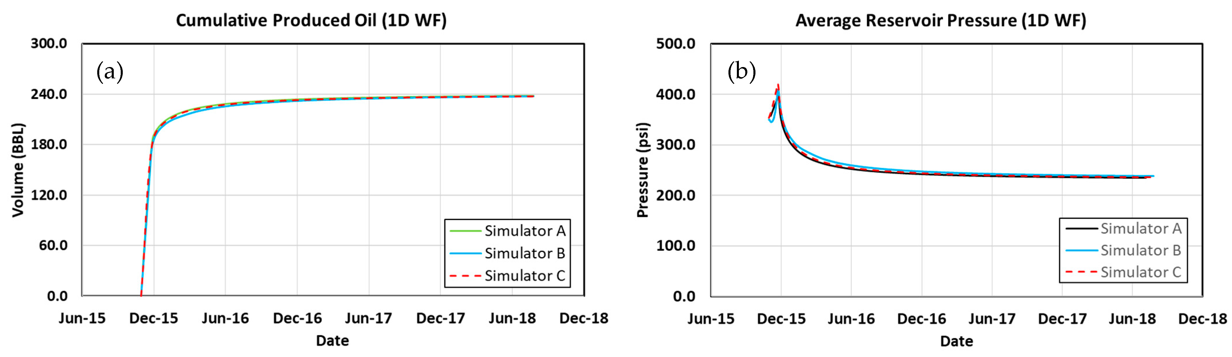
3.2. Waterflood
3.3. Polymer Flood
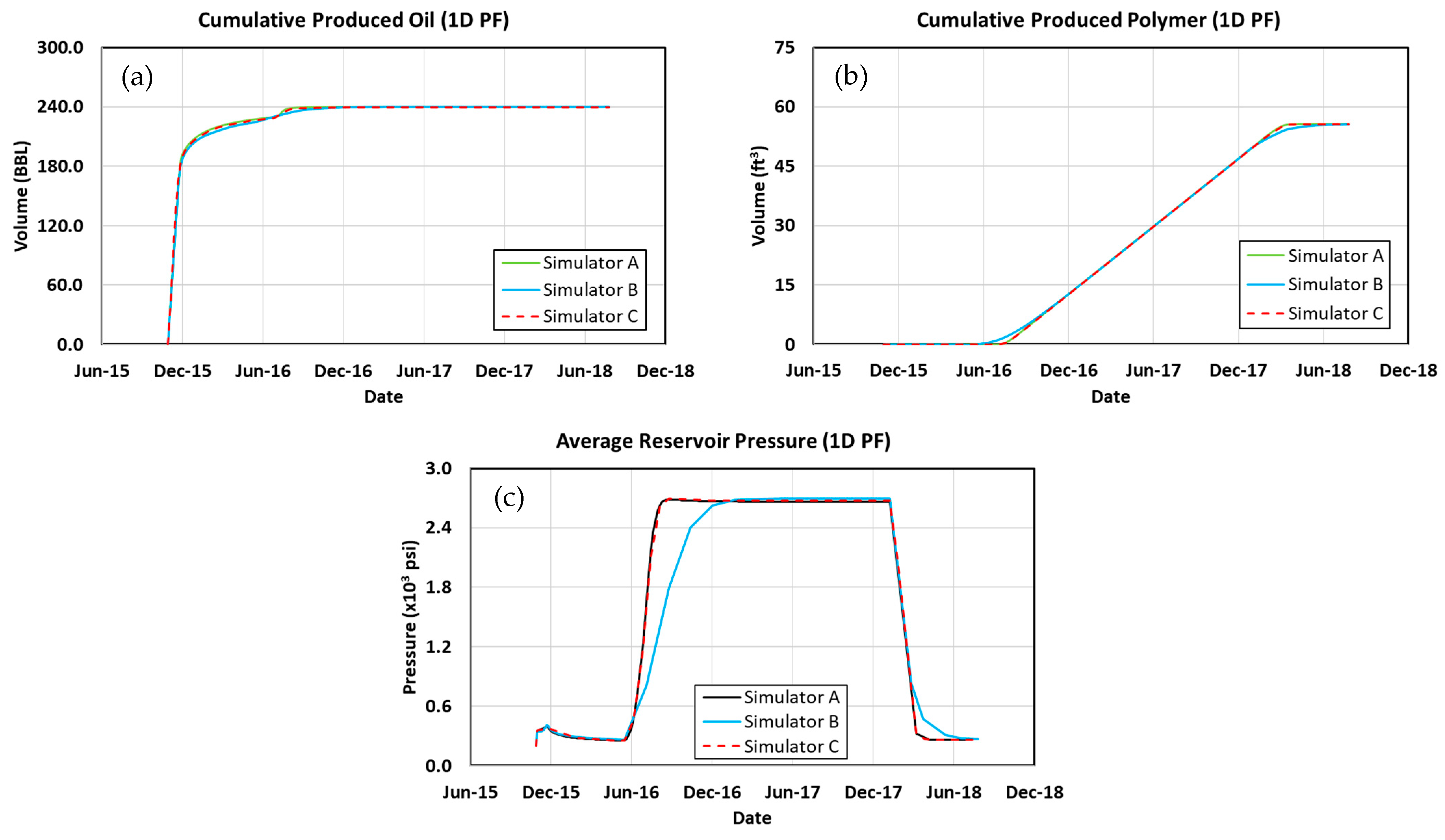
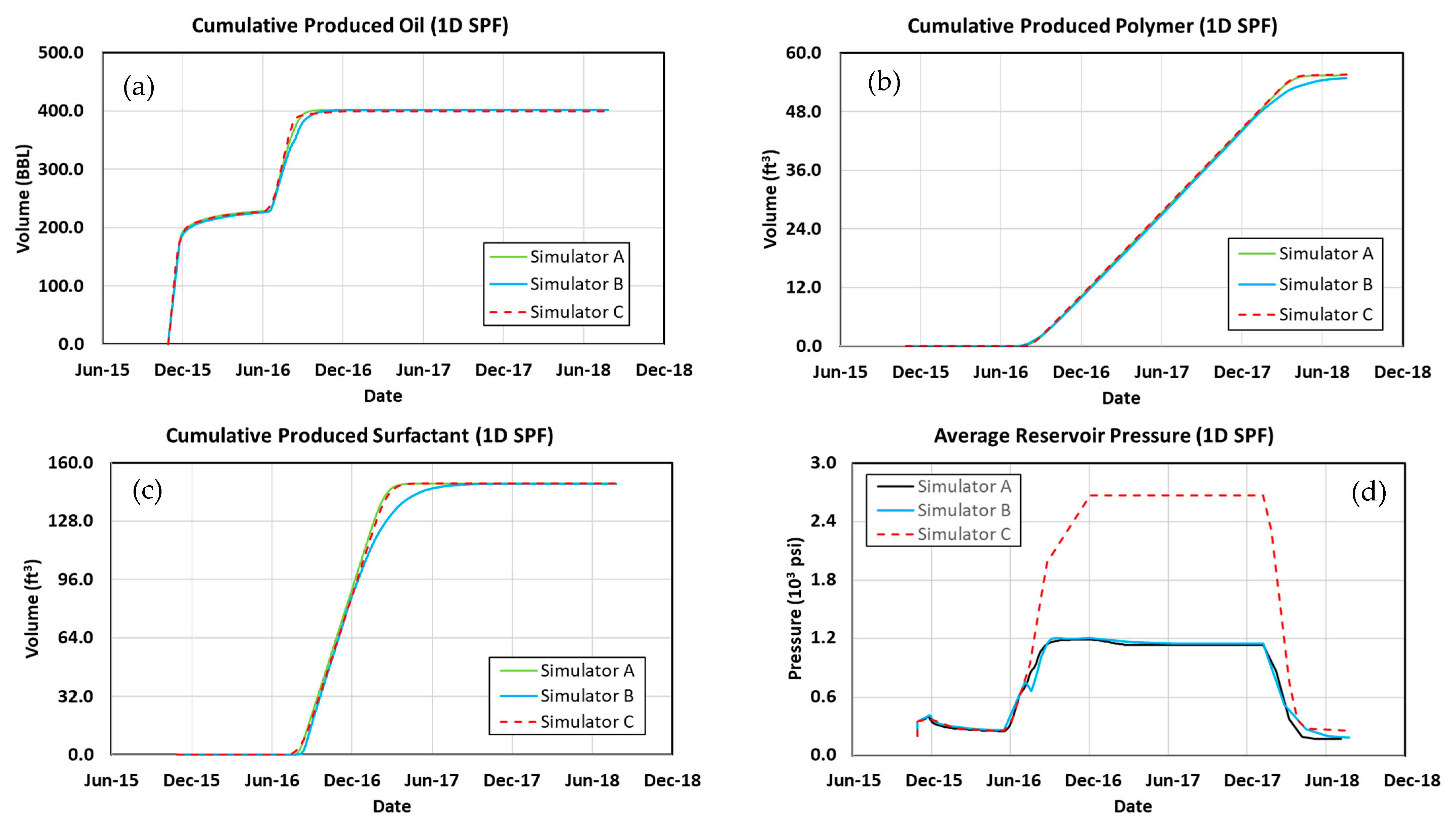
3.4. Surfactant–Polymer Flood
3.5. 3D Simulation Cases
3.6. Waterflood
3.7. Polymer Flood
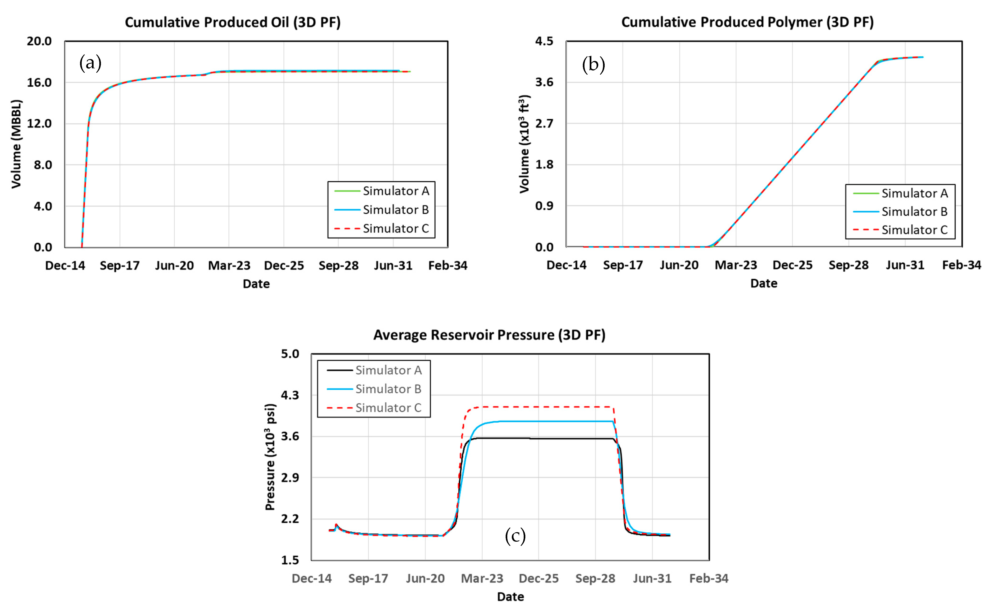
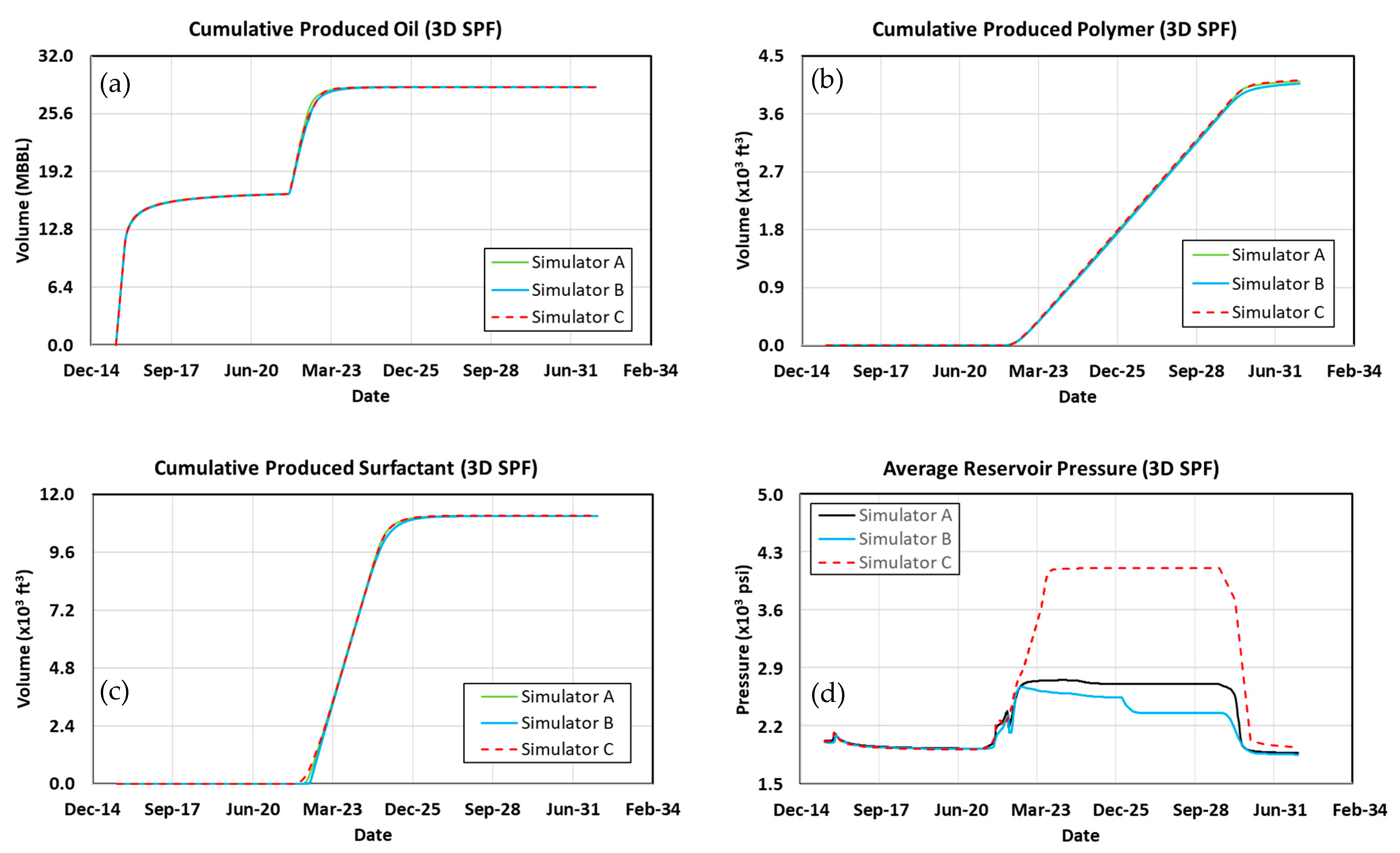
3.8. Surfactant–Polymer Flood
3.9. Field Model Simulations
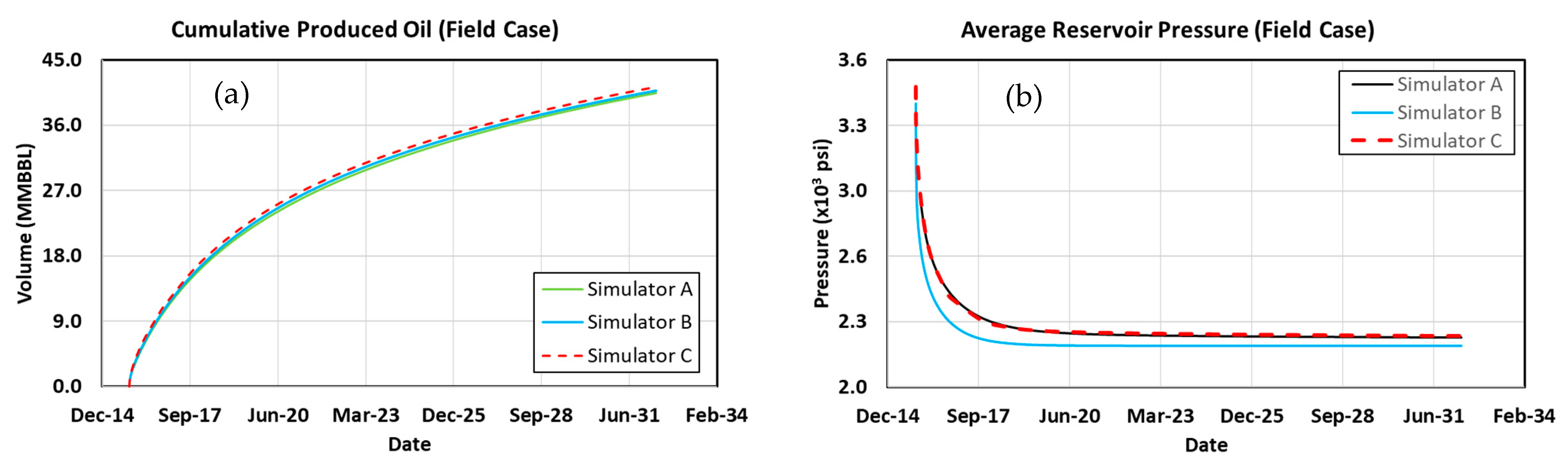
3.10. Waterflood
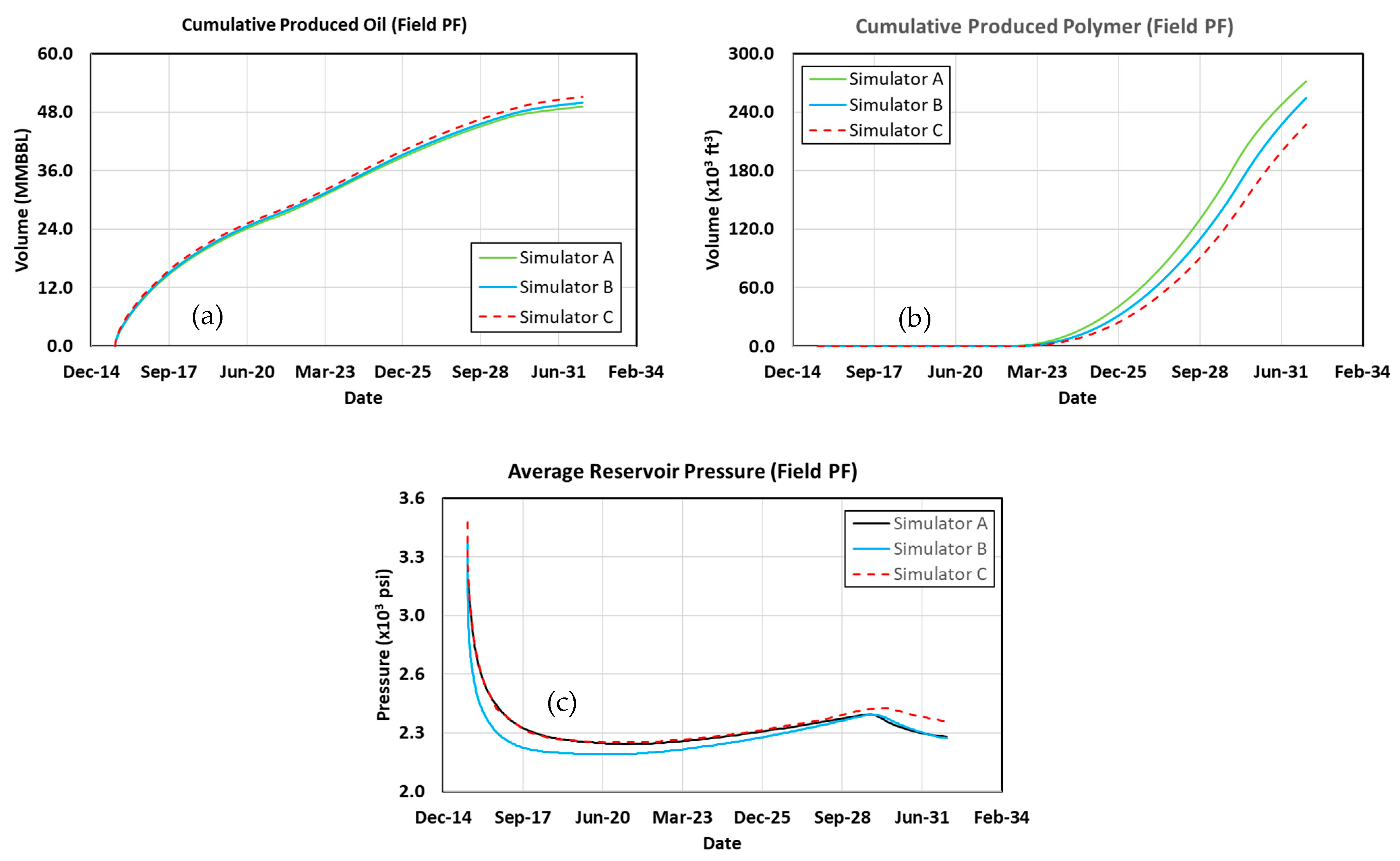
3.11. Polymer Flood
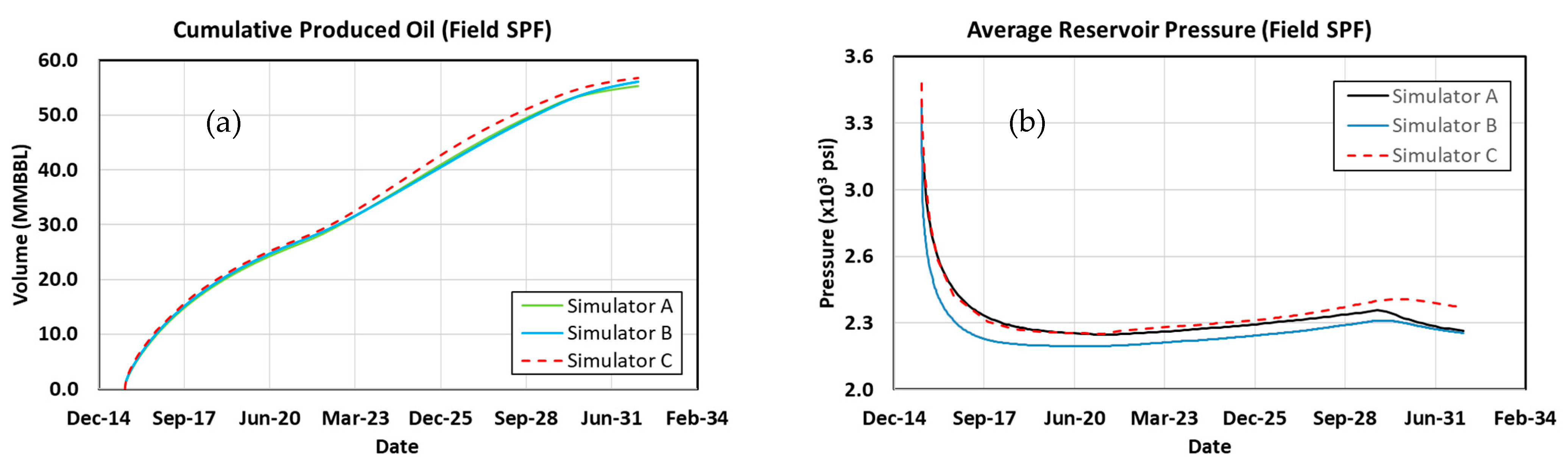
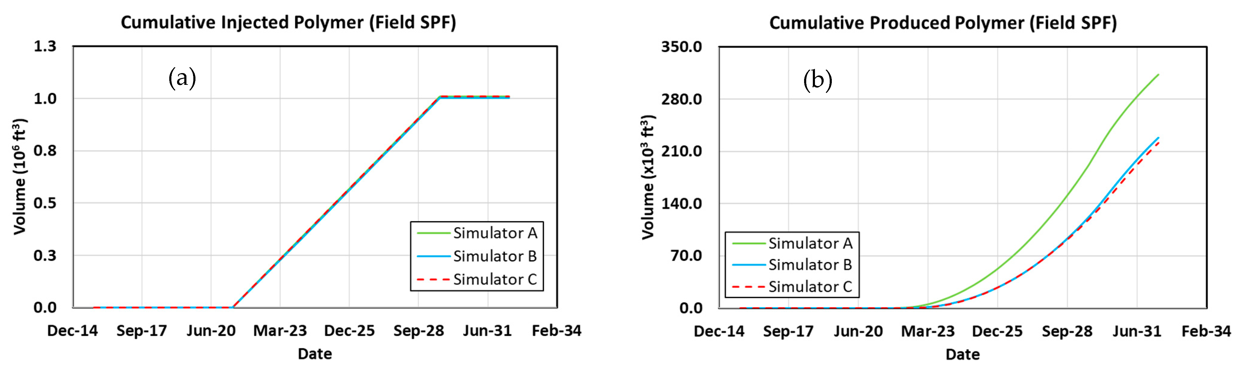
3.12. Surfactant–Polymer Flood
3.13. Comparing Results with Previous Work
4. Summary and Conclusions
Author Contributions
Funding
Data Availability Statement
Acknowledgments
Conflicts of Interest
Nomenclature
| The hydraulic potential gradient of the conjugate phase of phase ( | |
| Interfacial tension model parameter | |
| Parameter related to the height of the binodal curve for a given salinity | |
| Parameter related to the height of the binodal curve at zero salinity | |
| Parameter related to the height of the binodal curve at optimal salinity | |
| Parameter related to the height of the binodal curve at twice optimal salinity | |
| Polymer adsorption | |
| First fitting parameter for polymer solution viscosity at zero shear rate | |
| First fitting parameter for | |
| Second fitting parameter for polymer solution viscosity at zero shear rate | |
| Second fitting parameter for | |
| Third fitting parameter for polymer solution viscosity at zero shear rate | |
| Polymer’s adsorbed concentration obtained from the adsorption isotherm | |
| Adsorption of polymer using a Langmuir isotherm | |
| The maximum adsorption capacity of the rock | |
| B | Empirical parameters that define the binodal curves in Equation (A66) |
| Calibration parameter for the isotherm | |
| Permeability reduction input parameter | |
| Shear correction factor | |
| Interfacial tension model parameter | |
| The adsorbed polymer concentration | |
| The overall concentration of polymer | |
| The total anion concentration | |
| Total divalent cation concentration | |
| The concentration of oil in the microemulsion phase | |
| The oil concentration in the oleic phase | |
| The oil concentration in the aqueous phase | |
| Total polymer concentration | |
| Polymer concentration in the aqueous phase | |
| Polymer concentration in the microemulsion phase | |
| Maximum permeability reduction calibration parameter | |
| The effective salinity | |
| The optimum effective salinity | |
| The lower Type III effective salinity window values | |
| Effective salinity for polymer | |
| The upper Type III effective salinity window values | |
| The concentration of surfactant in the microemulsion phase | |
| The surfactant concentration in the oleic phase | |
| The surfactant concentration in the aqueous phase | |
| The total water concentration | |
| The concentration of water in the microemulsion phase | |
| The water concentration in the oleic phase | |
| The water concentration in the aqueous phase | |
| Phase term for computing the interfacial tension in Equation (A19) | |
| Depth | |
| Mixing function | |
| Hirasaki’s correction factor | |
| Interpolation parameter used for the microemulsion phase | |
| The gravity acceleration | |
| Reservoir permeability | |
| Geometric average of the permeability tensor | |
| The permeability tensor | |
| Reference permeability | |
| The relative permeability of phase ( | |
| The endpoint relative permeability of phase l ( | |
| The exponent of phase ( | |
| The relative permeability exponents for the aqueous oleic phase | |
| The trapping number of phase ( | |
| The relative permeability exponents for the aqueous phase | |
| Empirical coefficient | |
| Cutoff value for the permeability reduction | |
| Permeability reduction factor from phase l | |
| Maximum permeability reduction | |
| Permeability reduction | |
| The pseudo-phase l (w: water, o: oil) solubilization ratio | |
| The residual resistance factor of phase l | |
| The residual saturation of phase j (j | |
| The saturation of phase l ( | |
| The normalized saturation of phase ( | |
| The residual oil saturation | |
| Parameter for salinity slope | |
| The residual saturation of phase l ( | |
| The aqueous phase saturation | |
| The connate water saturation | |
| The trapping parameter of phase ( | |
| Function to calculate water relative permeability | |
| Function to calculate oil-water relative permeability | |
| First input parameter for | |
| Second input parameter for | |
| Third input parameter for | |
| Norm of the velocity of the aqueous phase | |
| Interpolation parameter in Equations (A34)–(A37) | |
| Component mole fraction | |
| The salinity | |
| First microemulsion viscosity from laboratory experiments | |
| Second microemulsion viscosity from laboratory experiments | |
| Third microemulsion viscosity from laboratory experiments | |
| Fourth microemulsion viscosity from laboratory experiments | |
| Fifth microemulsion viscosity from laboratory experiments | |
| Parameter for accounting for divalent cations | |
| The shear rate at which the polymer viscosity is equal to the average of and | |
| Parameter for computing as a function of polymer concentration | |
| Parameter for computing as a function of polymer concentration | |
| Polymer shear correction | |
| Equivalent shear rate | |
| Component viscosity | |
| The microemulsion viscosity | |
| Polymer viscosity | |
| Polymer viscosity | |
| Polymer solution viscosity at zero shear rate | |
| Water viscosity | |
| The mass density of conjugate phase l ( | |
| The mass density of phase l ( | |
| The interfacial tension between the phase l ( and its conjugate phase | |
| The interfacial tension between the displacing phase and the displaced phase ( | |
| Interfacial tension between the pseudo-phase l (w: water, o: oil) and the microemulsion phase | |
| The water-oil interfacial tension | |
| Interfacial tension used to calculate the microemulsion trapping number | |
| Porosity | |
| Superscript | |
| Property at either low or high trapping number | |
| Critical | |
| Property at high trapping number | |
| Property at low trapping number | |
| Oil-water | |
| Water | |
| Oil-water relative permeability | |
| water relative permeability | |
| Cell value of the oil-water relative permeability | |
| Cell value of the water relative permeability | |
| Subscript | |
| Critical | |
| Maximum | |
| Residual microemulsion | |
| Residual water | |
| Microemulsion | |
| Aqueous phase | |
| Oleic phase | |
| Residual oil | |
Appendix A. Model Description
Appendix A.1. Polymer-Related Properties
Appendix A.1.1. Viscosity
Appendix A.1.2. Polymer Rheology
Appendix A.1.3. Permeability Reduction
Appendix A.1.4. Adsorption
Appendix A.1.5. Oil/Water Relative Permeability
Appendix A.2. Surfactant
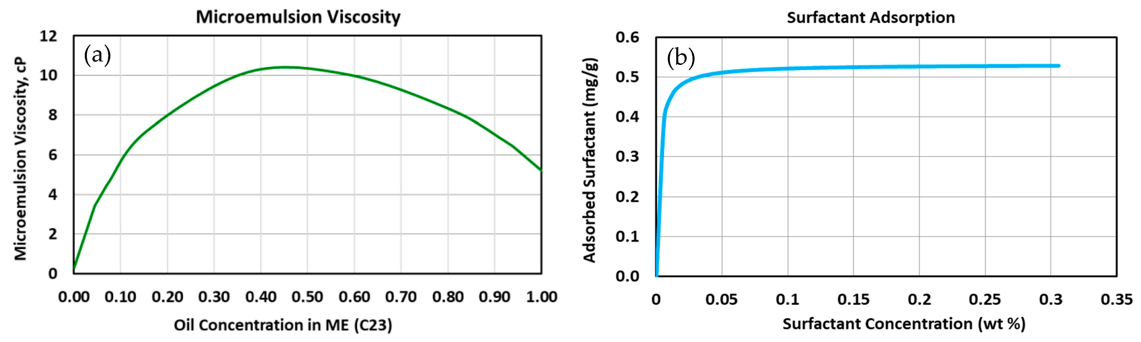
Appendix A.2.1. Microemulsion Viscosity
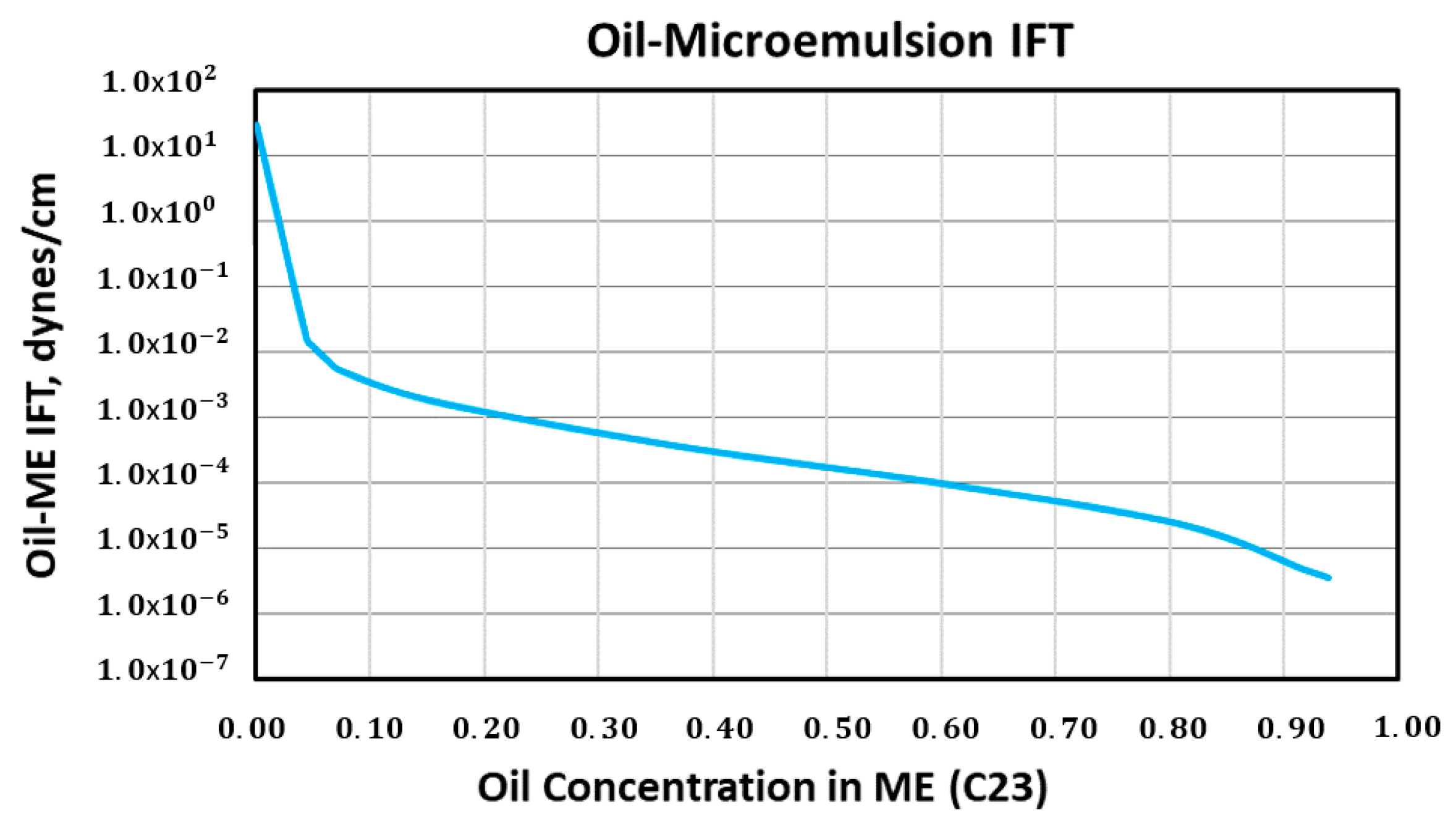
Appendix A.2.2. Interfacial Tension
Appendix A.2.3. Relative Permeability
Appendix A.2.4. Phase Behavior
References
- Vishnyakov, V.; Suleimanov, B.; Salmanov, A.; Zeynalov, E. Primer on Enhanced Oil Recovery; Gulf Professional Publishing: Cambridge, MA, USA, 2020; ISBN 978-0-12-817632-0. [Google Scholar]
- Green, D.W.; Willhite, G.P. Enhanced Oil Recovery; SPE textbook series; Henry, L., Ed.; Doherty Memorial Fund of AIME, Society of Petroleum Engineers: Richardson, TX, USA, 1998; ISBN 978-1-55563-077-5. [Google Scholar]
- Lake, L.W.; Johns, R.; Rossen, B.; Pope, G. Fundamentals of Enhanced Oil Recovery, 2nd ed.; Society of Petroleum Engineers: Richardson, TX, USA, 2014; ISBN 978-1-61399-328-6. [Google Scholar]
- Craig, F.F. The Reservoir Engineering Aspects of Waterflooding; Henry, L., Ed.; Doherty series; Doherty Memorial Fund of AIME: Richardson, TX, USA, 1993; ISBN 978-0-89520-202-4. [Google Scholar]
- Dake, L.P. Fundamentals of Reservoir Engineering; Developments in petroleum science; Elsevier Scientific Pub. Co.: Amsterdam, The Netherlands; Distributors for the U.S. and Canada Elsevier North-Holland: New York, NY, USA, 1978; ISBN 978-0-444-41667-4. [Google Scholar]
- Clifford, P.J.; Sorbie, K.S. The Effects of Chemical Degradation on Polymer Flooding. In Proceedings of the SPE Oilfield and Geothermal Chemistry Symposium, Phoenix, AZ, USA, 9–11 April 1985. [Google Scholar]
- Thomas, S. Enhanced Oil Recovery—An Overview. Oil Gas Sci. Technol. Rev. IFP 2008, 63, 9–19. [Google Scholar] [CrossRef] [Green Version]
- Griffin, W.C. Classification of Surface-Active Agents by “HLB”. J. Soc. Cosmet. Chem. 1949, 1, 311–326. [Google Scholar]
- Bourrel, M.; Schechter, R.S. Microemulsions and Related Systems: Formulation, Solvency, and Physical Properties; Surfactant science series; M. Dekker: New York, NY, USA, 1988; ISBN 978-0-8247-7951-1. [Google Scholar]
- Huh, C. Interfacial Tensions and Solubilizing Ability of a Microemulsion Phase That Coexists with Oil and Brine. J. Colloid Interface Sci. 1979, 71, 408–426. [Google Scholar] [CrossRef]
- Baran, J.R. Winsor I⇔;III⇔II Microemulsion Phase Behavior of Hydrofluoroethers and Fluorocarbon/Hydrocarbon Catanionic Surfactants. J. Colloid Interface Sci. 2001, 234, 117–121. [Google Scholar] [CrossRef] [PubMed]
- Ahmed, S.; Elraies, K.A. Microemulsion in Enhanced Oil Recovery. In Science and Technology Behind Nanoemulsions; Karakuş, S., Ed.; InTech: London, UK, 2018; ISBN 978-1-78923-570-8. [Google Scholar]
- Coats, K.H. An Equation of State Compositional Model. SPE J. 1980, 20, 363–376. [Google Scholar] [CrossRef]
- Acs, G.; Doleschall, S.; Farkas, E. General Purpose Compositional Model. SPE J. 1985, 25, 543–553. [Google Scholar] [CrossRef]
- Young, L.C.; Stephenson, R.E. A Generalized Compositional Approach for Reservoir Simulation. SPE J. 1983, 23, 727–742. [Google Scholar] [CrossRef]
- Collins, D.A.; Nghiem, L.X.; Li, Y.-K.; Grabonstotter, J.E. An Efficient Approach to Adaptive- Implicit Compositional Simulation With an Equation of State. SPE Reserv. Eng. 1992, 7, 259–264. [Google Scholar] [CrossRef]
- Watts, J.W. A Compositional Formulation of the Pressure and Saturation Equations. SPE Reserv. Eng. 1986, 1, 243–252. [Google Scholar] [CrossRef]
- Fernandes, B.R.B.; Marcondes, F.; Sepehrnoori, K. A New Four-Phase Adaptive Implicit Method for Compositional Reservoir Simulation. J. Comput. Phys. 2021, 435, 110263. [Google Scholar] [CrossRef]
- Fernandes, B.R.B.; Marcondes, F.; Sepehrnoori, K. Development of a Fully Implicit Approach with Intensive Variables for Compositional Reservoir Simulation. J. Pet. Sci. Eng. 2018, 169, 317–336. [Google Scholar] [CrossRef]
- Nogueira, R.L.; Fernandes, B.R.B.; Araújo, A.L.S.; Marcondes, F. Unstructured Grids and an Element Based Conservative Approach for a Black-Oil Reservoir Simulation. In Proceedings of the 13th Brazilian Congress of Thermal Sciences and Engineering, Uberlândia, Brazil, 5–10, December 2010. [Google Scholar]
- Haukas, J.; Aavatsmark, I.; Espedal, M.; Aavatsmark, I.; Espedal, M. A Black-Oil and Compositional IMPSAT Simulator with Improved Compositional Convergence. In Proceedings of the Proceedings of the 9th European Conference on the Mathematics of Oil Recovery, Cannes, France, 30 August–2 September 2004. [Google Scholar]
- CMG. GEM User Guide; CMG: Calgary, AB, Canada, 2022. [Google Scholar]
- CMG. IMEX User Guide; CMG: Calgary, AB, Canada, 2022. [Google Scholar]
- Schlumberger. Eclipse Reference Manual; Schlumberger: Houston, TX, USA, 2016. [Google Scholar]
- Nelson, R.C.; Pope, G.A. Phase Relationships in Chemical Flooding. SPE J. 1978, 18, 325–338. [Google Scholar] [CrossRef]
- Acosta, E.; Szekeres, E.; Sabatini, D.A.; Harwell, J.H. Net-Average Curvature Model for Solubilization and Supersolubilization in Surfactant Microemulsions. Langmuir 2003, 19, 186–195. [Google Scholar] [CrossRef]
- Khorsandi, S.; Johns, R.T. Robust Flash Calculation Algorithm for Microemulsion Phase Behavior. J. Surfactants Deterg. 2016, 19, 1273–1287. [Google Scholar] [CrossRef]
- Fernandes, B.R.B.; Sepehrnoori, K.; Delshad, M. Challenges in Modeling Microemulsion Phase Behavior. J. Surfact Deterg. 2022, 26, 311–333. [Google Scholar] [CrossRef]
- Pope, G.A.; Nelson, R.C. A Chemical Flooding Compositional Simulator. SPE J. 1978, 18, 339–354. [Google Scholar] [CrossRef]
- Delshad, M.; Pope, G.A.; Sepehrnoori, K. A Compositional Simulator for Modeling Surfactant Enhanced Aquifer Remediation, 1 Formulation. J. Contam. Hydrol. 1996, 23, 303–327. [Google Scholar] [CrossRef]
- Tong, S.; Chen, J. Full Implicit Numerical Simulator for Polymer Flooding and Profile Control. Int. J. Numer. Anal. Model. 2005, 2, 138–142. [Google Scholar]
- John, A.; Han, C.; Delshad, M.; Pope, G.A.; Sepehrnoori, K. A New Generation Chemical Flooding Simulator. SPE J. 2005, 10, 206–216. [Google Scholar] [CrossRef] [Green Version]
- Han, C.; Delshad, M.; Sepehrnoori, K.; Pope, G.A. A Fully Implicit, Parallel, Compositional Chemical Flooding Simulator. SPE J. 2007, 12, 322–338. [Google Scholar] [CrossRef]
- Winsor, P.A. Solvent Properties of Amphiphilic Compounds; Butterworths Scientific Publications: London, UK, 1954. [Google Scholar]
- Hand, D.B. Dineric Distribution. J. Phys. Chem. 1929, 34, 1961–2000. [Google Scholar] [CrossRef]
- Han, C.; Delshad, M.; Pope, G.A.; Sepehrnoori, K. Coupling Equation-of-State Compositional and Surfactant Models in a Fully Implicit Parallel Reservoir Simulator Using the Equivalent-Alkane-Carbon-Number Concept. SPE J. 2009, 14, 302–310. [Google Scholar] [CrossRef]
- Najafabadi, N.F.; Delshad, M.; Han, C.; Sepehrnoori, K. Formulations for a Three-Phase, Fully Implicit, Parallel, EOS Compositional Surfactant–Polymer Flooding Simulator. J. Pet. Sci. Eng. 2012, 86–87, 257–271. [Google Scholar] [CrossRef]
- Patacchini, L.; de Loubens, R.; Moncorge, A.; Trouillaud, A. Four-Fluid-Phase, Fully Implicit Simulation of Surfactant Flooding. SPE Reserv. Eval. Eng. 2014, 17, 271–285. [Google Scholar] [CrossRef]
- Yang, J.; Jin, B.; Jiang, L.; Liu, F. An Improved Numerical Simulator for Surfactant/Polymer Flooding. In Proceedings of the SPE/IATMI Asia Pacific Oil & Gas Conference and Exhibition, Nusa Dua, Bali, Indonesia, 20–22 October 2015; Society of Petroleum Engineers: Nusa Dua, Bali, Indonesia, 2015. [Google Scholar]
- Mykkeltvedt, T.S.; Raynaud, X.; Lie, K.A. Fully Implicit Higher-Order Schemes Applied to Polymer Flooding. Comput. Geosci. 2017, 21, 1245–1266. [Google Scholar] [CrossRef]
- Goudarzi, A.; Delshad, M.; Sepehrnoori, K. A Chemical EOR Benchmark Study of Different Reservoir Simulators. Comput. Geosci. 2016, 94, 96–109. [Google Scholar] [CrossRef]
- Nghiem, L.; Skoreyko, F.; Gorucu, S.E.; Dang, C.; Shrivastava, V. A Framework for Mechanistic Modeling of Alkali-Surfactant-Polymer Process in an Equation-of-State Compositional Simulator. In Proceedings of the SPE Reservoir Simulation Conference, Montgomery, TX, USA, 20–22 February 2017. [Google Scholar]
- Jong, S.; Nguyen, N.M.; Eberle, C.M.; Nghiem, L.X.; Nguyen, Q.P. Low Tension Gas Flooding as a Novel EOR Method: An Experimental and Theoretical Investigation. In Proceedings of the All Days; SPE: Tulsa, OK, USA, 2016; p. SPE-179559-MS. [Google Scholar]
- Shi, X.; Han, C.; Wolfsteiner, C.; Chang, Y.-B.; Schrader, M. A Mixed Natural and Concentration Variable Formulation for Chemical Flood Simulation. In Proceedings of the SPE Reservoir Simulation Conference, Montgomery, TX, USA, 20–22 February 2017; Society of Petroleum Engineers: Montgomery, TX, USA, 2017. [Google Scholar]
- Han, C.; Shi, X.; Chang, Y.-B.; Wolfsteiner, C.; Guyaguler, B. Modeling of Cosolvents in a Fully-Implicit Surfactant Flood Simulator Using the Three-Level Framework. In Proceedings of the SPE Reservoir Simulation Conference, Galveston, TX, USA, 10–11 April 2019; Society of Petroleum Engineers: Galveston, TX, USA, 2019. [Google Scholar]
- Jia, Z.; Li, D.; Xue, Z.; Lu, D. Development of a Fully Implicit Simulator for Surfactant-Polymer Flooding by Applying the Variable Substitution Method. Int. J. Oil Gas Coal Technol. 2019, 21, 1. [Google Scholar] [CrossRef]
- Fernandes, B.R.B. Development of Adaptive Implicit Chemical and Compositional Reservoir Simulators. Ph.D. Thesis, The University of Texas at Austin, Austin, TX, USA, 2019. [Google Scholar]
- Fernandes, B.R.B.; Sepehrnoori, K.; Delshad, M.; Marcondes, F. New Fully Implicit Formulations for the Multicomponent Surfactant-Polymer Flooding Reservoir Simulation. Appl. Math Model 2022, 105, 751–799. [Google Scholar] [CrossRef]
- Guzman, J.A.N.; Fernandes, B.R.B.; Delshad, M.; Sepehrnoori, K.; Zapata, J.F. Evaluation of Polymer Flooding in a Highly Stratified Heterogeneous Reservoir. A Field Case Study. Wseas Trans. Environ. Dev. 2020, 16, 23–33. [Google Scholar] [CrossRef]
- Schlumberger. Intersect User Guide; Schlumberger: Houston, TX, USA, 2020. [Google Scholar]
- CMG. STARS User Guide; CMG: Calgary, AB, Canada, 2022. [Google Scholar]
- Equinor Volve Field Data (CC BY-NC-SA 4.0). Available online: https://www.equinor.com/news/archive/14jun2018-disclosing-volve-data (accessed on 8 April 2023).
- Druetta, P.; Picchioni, F. Surfactant flooding: The Influence of the Physical Properties on the Recovery Efficiency. Petroleum 2020, 6, 149–162. [Google Scholar] [CrossRef]
- Lashgari, H.R.; Sepehrnoori, K.; Delshad, M.; DeRouffignac, E. Development of a four-phase chemical-gas model in an Impec Reservoir simulator. In Proceedings of the Day 1 Mon, Houston, TX, USA, 23–25 February 2015. SPE Reservoir Simulation Symposium. [Google Scholar] [CrossRef]
- Flory, P.J. Principles of Polymer Chemistry; Cornell University Press: Ithaca, NY, USA, 1953; ISBN 978-0-8014-0134-3. [Google Scholar]
- Lake, L.W. Enhanced Oil Recovery; Society of Petroleum Engineers: Richardson, TX, USA, 2010; ISBN 978-1-55563-305-9. [Google Scholar]
- Delshad, M. A Study of Transport of Micellar Fluids in Porous Media. Ph.D. Dissertation, The University of Texas at Austin, Austin, TX, USA, 1986. [Google Scholar]
- Carreau, P.J. Rheological Equations from Molecular Network Theories. Trans. Soc. Rheol. 1972, 16, 99–127. [Google Scholar] [CrossRef]
- Meter, D.M.; Bird, R.B. Tube Flow of Non-Newtonian Polymer Solutions: Part I. Laminar Flow and Rheological Models. AIChE J. 1964, 10, 878–881. [Google Scholar] [CrossRef]
- Hirasaki, G.J.; Pope, G.A. Analysis of Factors Influencing Mobility and Adsorption in the Flow of Polymer Solution Through Porous Media. Soc. Pet. Eng. J. 1974, 14, 337–346. [Google Scholar] [CrossRef]
- Lin, E. A Study of Micellar/Polymer Flooding Using a Compositional Simulator. PhD Thesis, The University of Texas at Austin, Austin, TX, USA, 1981. [Google Scholar]
- Al-Rawahi, H.; Delshad, M.; Sepehrnoori, K.; Al-Kindy, A. Modeling Approach and Non-Uniqueness of Polymer Coreflood History Match and Field-Scale Forecasts. In Proceedings of the Day 1 Mon, Abu Dhabi, United Arab Emirates, 9 November 2020; SPE: Abu Dhabi, United Arab Emirates, 2020; p. D012S116R098. [Google Scholar]
- Hirasaki, G.J. Application of the Theory of Multicomponent, Multiphase Displacement to Three-Component, Two-Phase Surfactant Flooding. Soc. Pet. Eng. J. 1981, 21, 191–204. [Google Scholar] [CrossRef]
- Delshad, M. Trapping of Micellar Fluids in Berea Sandstone. Ph.D. Thesis, The University of Texas at Austin, Austin, TX, USA, 1990. [Google Scholar]
- Jin, M. A Study of Nonaqueous Phase Liquid Characterization and Surfactant Remediation. Ph.D. Thesis, The University of Texas at Austin, Austin, TX, USA, 1995. [Google Scholar]
- Delshad, M.; Bhuyan, D.; Pope, G.A.; Lake, L.W. Effect of Capillary Number on the Residual Saturation of a Three-Phase Micellar Solution. In Proceedings of the SPE Enhanced Oil Recovery Symposium, Tulsa, Oklahoma, 20–23 April 1986; Society of Petroleum Engineers: Tulsa, Oklahoma, 1986. [Google Scholar]
- Healy, R.N.; Reed, R.L.; Stenmark, D.G. Multiphase Microemulsion Systems. SPE J. 1976, 16, 147–160. [Google Scholar] [CrossRef]


| Model | 1-Dimensional Cartesian |
|---|---|
| Grid Size | 15 × 1 × 1 Grids |
| Grid Dimensions | 10 × 10 × 10 ft for each grid |
| Wells | One injector and one producer |
| Injection Constraint | Rate = 3.75 ft3/day |
| Production Constraint | BHP = 120 psi |
| Initial Water Saturation | 0.25 |
| Initial Pressure | 200 psi |
| Permeability | 100 mD |
| Porosity | 0.2 |
| Rock Compressibility | 10−6 psi−1 @200 psi Ref. Pressure |
| Reference Pressure | 200 psi |
| Model | 3-Dimensional Cartesian Model |
|---|---|
| Grid Size | 15 × 15 × 10 |
| Grid Dimensions | 10 × 10 × 10 ft |
| Wells | One injector and one producer |
| Injection Constraint | 100 bbls/day |
| Production Constraint | BHP = 1800 psi |
| Initial Water Saturation | 0.25 |
| Initial Pressure | 2000 psi |
| Permeability | Isotropic 100 mD |
| Porosity | 0.19 |
| Rock Compressibility | 1/psi @ Ref Pressure of 2000 psi |
| Model | 3-Dimensional Corner Grid Point Model |
|---|---|
| No. of Grids | 108 × 100 × 63 |
| Wells | 12 injectors and 6 producers |
| Injection Constraint | 2000 bbls/day |
| Production Constraint | BHP = 1800 psi |
| Average Initial Water Sat. | 0.56 |
| Average Initial Pressure | 3417 psi |
| Permeability | X and Y: 0.01 min, 23,381 max, 1348 average mDZ: 0.0001 min, 9352 max, 505 average mD |
| Porosity | 0.01 min, 0.2987 max, 0.2 average |
| Rock Compressibility | 1/psi @ Ref pressure of 2000 psi |
| Parameter | Value |
|---|---|
| Water Specific Gravity | 0.433 psi/ft |
| Oil Specific Gravity | 0.368 psi/ft |
| Water and Oil Viscosities | 1 cP, 5.2 cP |
| Residual Water Saturation () | 0.25 |
| Residual Oil Saturation () | 0.3 |
| Endpoint Water Relative Permeability () | 0.4 |
| Endpoint Oil Relative Permeability () | 1 |
| Water and Oil Exponents () | 3, 1.8 |
| Polymer Model | Simulator A | Simulator B | Simulator C |
|---|---|---|---|
| Viscosity as a Function of Polymer Concentration | 1 | 1 | 2 |
| Viscosity as a Function Shear Rate | 1 | 1 | 2 |
| Effect of Salinity on Polymer Properties | 1 | 1 | 2 |
| Adsorption | 1 | 1 1 | 2 |
| Permeability Reduction | 1 | 1 | 2 |
| Parameter | Value |
|---|---|
| Viscosity Parameter () | 12.54 |
| Viscosity Parameter () | 41 |
| Viscosity Parameter () | 715 |
| Effective Salinity | 0.1 meq/mL |
| Salinity Parameter | 0 |
| Adsorption Parameter () | 3.1 |
| Adsorption Parameter () | 0 |
| Adsorption Parameter () | 100 |
| Perm. Reduction () | 0.0186 |
| Perm. Reduction () | 1000 |
| Perm. Reduction Cutoff | 10 |
| Surfactant Model | Simulator A | Simulator B | Simulator C |
|---|---|---|---|
| Microemulsion Viscosity | 1 | 1 | Not Included |
| Adsorption | 1 | 1 | 2 |
| Binodal Curve for Microemulsion Phase Behavior | 1 | 1 | Not Included |
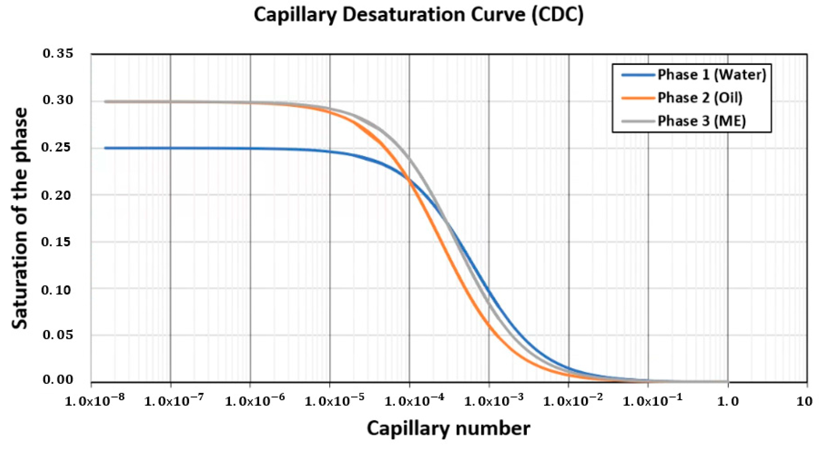
| Capillary Desaturation Curve | 1 | 1 1 | Not Included |
| Interfacial Tension | 1 | 1 | 2 |
| Relative Permeability | 1 | 2 | 3 |
| Parameter | Value |
|---|---|
| Microemulsion Viscosity Parameter () | 2.5 |
| Microemulsion Viscosity Parameter () | 2.3 |
| Microemulsion Viscosity Parameter (), cP | 10 |
| Microemulsion Viscosity Parameter () | 1 |
| Microemulsion Viscosity Parameter () | 1 |
| Surfactant Adsorption Parameter () | 0.3 |
| Surfactant Adsorption Parameter () | 0 |
| Surfactant Adsorption Parameter () | 500 |
| Lower Limit of Effective Salinity (), meq/mL | 0.177 |
| Upper Limit of Effective Salinity (), meq/mL | 0.344 |
| Height of Binodal Curve at Zero Effective Salinity | 0.131 |
| Height of Binodal Curve at Optimum Effective Salinity | 0.026 |
| Height of Binodal Curve at Twice Optimum Effective Salinity | 0.028 |
| Water Trapping Parameter () | 1600 |
| Oil Trapping Parameter () | 4000 |
| Microemulsion Trapping Parameter () | 2600 |
| Swr at High Trapping Number (water phase) | 0 |
| Sor at High Trapping Number (oil phase) | 0 |
| Smr at High Trapping Number (microemulsion phase) | 0 |
| Huh Interfacial Tension Constant () | 0.35 |
| Huh Interfacial Tension Constant () | 10 |
| % Difference | |||
|---|---|---|---|
| Simulator B/C | Simulator A/C | Simulator A/B | |
| Cum. Fluid inj. | 0.000% | 0.000% | 0.000% |
| Prod. Volume of water | −0.006% | −0.012% | −0.005% |
| Prod. Oil Volume | 0.154% | 0.299% | 0.145% |
| Total Fluid Produced | −0.001% | 0.000% | 0.000% |
| % Difference | |||
|---|---|---|---|
| Simulator B/C | Simulator A/C | Simulator A/B | |
| Cum. Inj. Fluid | 0.000% | 0.000% | 0.000% |
| Prod. Water Volume | −0.008% | −0.006% | 0.002% |
| Volume of Oil Prod. | 0.293% | 0.257% | −0.036% |
| Polymer Inj. | 0.000% | 0.000% | 0.000% |
| Polymer Prod. | −0.048% | 0.107% | 0.156% |
| Total Fluid Prod. | 0.003% | 0.004% | 0.001% |
| % Difference | |||
|---|---|---|---|
| Simulator B/C | Simulator A/C | Simulator A/B | |
| Cum. Inj. Fluid | 0.000% | 0.000% | 0.000% |
| Produced Water Volume | 0.011% | −0.011% | −0.023% |
| Produced Oil Volume | 0.323% | 0.281% | −0.042% |
| Polymer Inj. | −0.651% | 0.020% | 0.667% |
| Polymer Prod. | −1.299% | 0.156% | 1.437% |
| Surfactant Inj. | 0.006% | 0.006% | 0.000% |
| Surfactant Prod. | −0.098% | −0.053% | 0.045% |
| Total Fluid Prod. | 0.030% | 0.006% | −0.024% |
| % Difference | |||
|---|---|---|---|
| Simulator B/C | Simulator A/C | Simulator A/B | |
| Cum. Inj. Fluid | 0.000% | 0.000% | 0.000% |
| Produced Water Volume | −0.005% | 0.002% | 0.004% |
| Produced Oil Volume | 0.127% | 0.065% | −0.061% |
| Total Fluid Prod. | −0.002% | 0.000% | 0.002% |
| % Difference | |||
|---|---|---|---|
| Simulator B/C | Simulator A/C | Simulator A/B | |
| Cum. Inj. Fluid | 0.000% | 0.000% | 0.000% |
| Produced Water Volume | −0.022% | 0.001% | 0.022% |
| Produced Oil Volume | 0.489% | 0.025% | −0.466% |
| Volume of Polymer Inj. | 0.000% | 0.000% | 0.000% |
| Volume of Polymer Prod. | −0.062% | 0.032% | 0.093% |
| Total Fluid Prod. | −0.008% | 0.001% | 0.009% |
| % Difference | |||
|---|---|---|---|
| Simulator B/C | Simulator A/C | Simulator A/B | |
| Cum. Inj. Fluid | 0.000% | 0.000% | 0.000% |
| Produced Water Volume | −0.001% | −0.001% | 0.000% |
| Produced Oil Volume | 0.106% | 0.117% | 0.012% |
| Volume of Polymer Inj. | −0.651% | 0.020% | 0.667% |
| Volume of Polymer Prod. | −1.276% | −0.370% | 0.895% |
| Volume of Surfactant Inj. | 0.006% | 0.006% | 0.000% |
| Volume of Surfactant Prod. | −0.140% | −0.137% | 0.003% |
| Total Fluid Prod. Volumes | 0.004% | 0.005% | 0.000% |
| % Difference | |||
|---|---|---|---|
| Simulator B/C | Simulator A/C | Simulator A/B | |
| Cum. Inj. Fluid Volume | 0.000% | −0.001% | 0.000% |
| Produced Water Volume | −0.455% | −0.129% | −0.325% |
| Produced Oil Volume | −1.250% | −2.071% | −0.811% |
| Total Volume of Fluid Prod. | −0.675% | −0.660% | 0.014% |
| % Difference | |||
|---|---|---|---|
| Simulator B/C | Simulator A/C | Simulator A/B | |
| Cum. Inj. Fluid | 0.000% | 0.000% | 0.000% |
| Produced Water Volume | 1.028% | 1.715% | 0.694% |
| Produced Oil Volume | −2.379% | −4.043% | −1.625% |
| Polymer Inj. | 0.000% | 0.000% | 0.000% |
| Polymer Prod. | 10.661% | 16.243% | 6.248% |
| Total Fluid Prod. | −0.125% | −0.204% | −0.079% |
| % Difference | |||
|---|---|---|---|
| Simulator B/C | Simulator A/C | Simulator A/B | |
| Cum. Inj. Fluid Volume | 0.000% | 0.000% | 0.000% |
| Produced Water Volume | 0.228% | 1.235% | 1.010% |
| Produced Oil Volume | −1.210% | −2.670% | −1.442% |
| Polymer Inj. Volume | −0.671% | 0.000% | 0.667% |
| Polymer Prod. Volume | 3.057% | 29.28% | 27.049% |
| Surfactant Inj. Volume | 2.950% | 2.950% | 0.000% |
| Surfactant Prod. Volume | −130.361% | 1.357% | 57.179% |
| Total Fluid Prod. Volume | −0.319% | −0.227% | 0.092% |
Disclaimer/Publisher’s Note: The statements, opinions and data contained in all publications are solely those of the individual author(s) and contributor(s) and not of MDPI and/or the editor(s). MDPI and/or the editor(s) disclaim responsibility for any injury to people or property resulting from any ideas, methods, instructions or products referred to in the content. |
© 2023 by the authors. Licensee MDPI, Basel, Switzerland. This article is an open access article distributed under the terms and conditions of the Creative Commons Attribution (CC BY) license (https://creativecommons.org/licenses/by/4.0/).
Share and Cite
Alhotan, M.M.; Batista Fernandes, B.R.; Delshad, M.; Sepehrnoori, K. A Systemic Comparison of Physical Models for Simulating Surfactant–Polymer Flooding. Energies 2023, 16, 5702. https://doi.org/10.3390/en16155702
Alhotan MM, Batista Fernandes BR, Delshad M, Sepehrnoori K. A Systemic Comparison of Physical Models for Simulating Surfactant–Polymer Flooding. Energies. 2023; 16(15):5702. https://doi.org/10.3390/en16155702
Chicago/Turabian StyleAlhotan, Muhammad M., Bruno R. Batista Fernandes, Mojdeh Delshad, and Kamy Sepehrnoori. 2023. "A Systemic Comparison of Physical Models for Simulating Surfactant–Polymer Flooding" Energies 16, no. 15: 5702. https://doi.org/10.3390/en16155702